15.2 The housing market and residential con- struction

15.2. The housing market and residential construction 645

tween ρ and r, as long as the stability condition (15.44) is satisfied. Or, to bemore precise: the Blanchard model works well in the case ρ < r; in the oppo-site case, where ρ > r, the model works at least better than the Ramsey model,because it never implies that Ct → 0 in the long run.It should be admitted, however, that in the case of a very impatient coun-

try (ρ > r), even the OLG model implies a counterfactual prediction. What(15.47) tells us is that the impatient small open economy in a sense asymptot-ically mortgages all of its physical capital and part of its human capital. TheOLG model predicts this will happen, if financial markets are perfect, and if thepolitical sphere does not intervene. It certainly seems unlikely that an economicdevelopment, ending up with negative national wealth, is going to be observed inpractice. There are two - complementary - explanations of this.First, the international credit market is far from perfect. Because a full-scale

supranational legal authority comparable with domestic courts is lacking, creditdefault risk in international lending is generally a more serious problem than indomestic lending. Physical capital can to some extent be used as a collateralon foreign loans, while human wealth is not suitable. Human wealth cannot berepossessed. This implies a constraint on the ability to borrow.10 And lenders’risk perceptions depend on the level of debt.Second, long before all the physical capital of an impatient country is mort-

gaged or have directly become owned by foreigners, the government presumablywould intervene. In fear of losing national independence, it would use its politicalpower to end the pawning of economic resources to foreigners.This is a reminder, that we should not forget that the economic sphere of a

society is just one side of the society. Politics as well as culture and religion areother sides. The economic outcome may be conditioned on these social factors,and the interaction of all these spheres determines the final outcome.

15.2 The housing market and residential con-struction

The housing market is from a macroeconomic point of view important for severalreasons: a) housing makes up a substantial proportion of the consumption budget;b) housing wealth makes up a substantial part of private wealth of a major fraction

10We have been speaking as if domestic residents own the physical capital stock in the country,but have obtained part or all the financing of the stock by issuing bonds to foreigners. Theresults would not change if we allowed for foreign direct investment. Then foreigners wouldthemselves own part of the physical capital rather than bonds. In such a context a similarconstraint on foreign investment is likely to arise, since a foreigner can buy a factory or theshares issued by a firm, but it is diffi cult to buy someone else’s stream of future labour income.

c© Groth, Lecture notes in macroeconomics, (mimeo) 2016.

646CHAPTER 15. FURTHER APPLICATIONS OF

ADJUSTMENT COST THEORY

of the population; c) fluctuations in house prices and in construction activity arelarge and seem important for business cycles; and d) residential investment, whishtypically is of magnitude 5 percent of GDP, and aggregate output are stronglypositively correlated. The analysis will be based on a simple dynamic partialequilibrium model with rising marginal construction costs.Let time be continuous. Let Ht denote the aggregate housing stock at time

t and St the aggregate flow of housing services at time t. Ignoring heterogeneity,the housing stock can be measured in terms of m2 floor area at a given point intime. For convenience we will talk about the stock as a certain number of housesof a standardized size. The supply of housing services at time t constitute aflow, thereby being measured per time unit, say per year: so and so many squaremeter-months are at the disposal for accommodation during the year. The twoconcepts are related through

St = αHt, α > 0, (15.49)

where we will treat α as a constant which depends only on the measurement unitfor housing services. If these are measured in square meter-months, α equals thenumber of square meters of a “normal-sized”house times 12.We ignore population growth and economy-wide technological progress.

15.2.1 The housing service market and the house market

There are two goods, houses and housing services, and therefore also two marketsand two prices:

pt = the (real) price of a “normal-sized‘”house at time t,

Rt = the rental rate ≡ the (real) price of housing services at time t.

The price Rt of housing services is known as the rental rate at the housing market.Buying a housing service means renting the apartment or the house for a certainperiod. Or, if we consider an owner-occupied house (or apartment), Rt is theimputed rental rate, that is, the owner’s opportunity cost of occupying the house.The prices Rt and pt are measured in real terms, or more precisely, they aredeflated by the consumer price index. We assume perfect competition in bothmarkets.

The market for housing services

In the short run the housing stock is historically given. Construction is time-consuming and houses cannot be imported. Owing to the long life of houses,investment in new houses per year tends to be a small proportion of the available



housing stock (in advanced economies about 3 percent, say). So also the supply,St, of housing services is given in the short run.Suppose the aggregate demand for housing services at time t is

Sdt = D(Rt, A, PV (wL)), D1 < 0, D2 > 0, D3 > 0, (15.50)

where A is aggregate financial wealth and PV (wL) is human wealth, i.e., thepresent discounted value of expected future labor income after tax for those alive.That demand depends negatively on the rental rate reflects that both the sub-stitution effect and the income effect of a higher rental rate are negative. Thewealth effect on housing demand of a higher rental rate is likely to be positive forowners and negative for tenants.11

The market for housing services is depicted in Fig. 15.6. We get a characteri-zation of the equilibrium rental rate in the following way. In equilibrium at timet, Sdt = St, that is,

D(Rt, A, PV (wL)) = αHt. (15.51)

This equation determines Rt as an implicit function, Rt = R(Ht, A, PV (wL)),of Ht, A, and PV (wL). By implicit differentiation in (15.51) we find the partialderivatives of this function, RH = α/DR < 0, RA = −DA/DS > 0, and RPW

= −DPV /DR > 0.

The supply of housing services is inelastic in the short run and the marketclearing rental rate immediately moves up and down as the demand curve shiftsrightward or leftward. But in our partial equilibrium framework, we will considerA and PV (wL) as exogenous and constant. Hence we suppress these two variablesas arguments in the functions and define R(Ht) ≡ R(Ht, A, PV (wL)), whereby

Rt = R(Ht), R′ = α/DR < 0. (15.52)

From now on our time unit will be one year and we define one unit of housingservice per year to mean disposal of a house of standard size one year. By this,α in (15.49) equals 1.

11A simple microeconomic “rationale”behind the aggregate demand function (15.50) is ob-tained by assuming an instantaneous utility function u(ht, ct) = ln(hγt c

1−γt ), where 0 < γ < 1,

and ht is consumption of housing services at time t, whereas ct is non-housing consumption.Then the share of housing expenditures in the total instantaneous consumption budget is aconstant, γ. This is broadly in line with empirical evidence for the US (Davis and Heathcote,2005). In turn, according to standard neoclassical theory, the total consumption budget will bean increasing function of total wealth of the household, cf. Chapter 9. Separation between thetwo components of wealth, A and PV (wl), is relevant when credit markets are imperfect.




Figure 15.6: Supply and demand in the market for housing services at time t.

The market for existing houses

Because a house is a durable good with market value, it is an asset. This assettypically constitutes a substantial share of the wealth of a large fraction of thepopulation, the house-owners. At the same time the supply of the asset canchange only slowly.Assume there is an exogenous and constant risk-free real interest rate r > 0.

This is a standard assumption in partial equilibrium analysis. If the economy isa small open economy with perfect capital mobility, the exogeneity of r (if notconstancy) is warranted even in general equilibrium analysis.Considering the asset motive associated with housing, a series of aspects are

central. We let houses depreciate physically at a constant rate δ > 0. Supposethere is a constant tax rate τR ∈ [0, 1) applied to rental income (possibly imputed)after allowance for depreciation. In case of an owner-occupied house the ownermust pay the tax τR(Rt − δpt) out of the imputed income (Rt − δpt) per houseper year. Assume further there is a constant property tax (real estate tax) τ p ≥ 0applied to the market value of houses. Finally, suppose that a constant tax rateτ r ∈ [0, 1) applies to interest income. There is symmetry in the sense that if youare a debtor and have negative interest income, then the tax acts as a rebate. Weassume capital gains are not taxed and we ignore all complications arising fromthe fact that most countries have tax systems based on nominal income ratherthan real income. In a low-inflation world this limitation may not be serious.12

Suppose there are no credit market imperfections, no transaction costs, and nouncertainty. Assume further that the user of housing services value these services

12Note, however, that if all capital income should be taxed at the same rate, capital gainsshould also be taxed at the rate τ r, and τR should equal τ r. In Denmark, in the early 2000s,the government replaced the rental value tax, τR, on owner-occupied houses by a lift in theproperty tax, τp. Since then, due to a nominal “tax freeze”, τp has been gradually decreasingin real terms.



independently of whether he/she owns or rent. Under these circumstances theprice of houses, pt, will adjust so that the expected after-tax rate of return onowning a house equals the after-tax rate of return on a safe bond. We thus havethe no-arbitrage condition

(1− τR)(R(Ht)− δpt)− τ ppt + petpt

= (1− τ r)r, (15.53)

where pet denotes the expected capital gain per time unit (so far pet is just a

commonly held subjective expectation).For given pet we find the equilibrium price

pt =(1− τR)R(Ht) + pet

(1− τ r)r + (1− τR)δ + τ p.

Thus pt depends on Ht, pet , r, and tax rates in the following way:

∂pt∂Ht

=(1− τR)R′(Ht)

(1− τ r)r + (1− τR)δ + τ p< 0,

∂pt∂pet

=1

(1− τ r)r + (1− τR)δ + τ p> 0,

∂pt∂τR

=− [(1− τ r)r + τ p]R(Ht) + δpet[(1− τ r)r + (1− τR)δ + τ p]

2 S 0 for pet S[(1− τ r)r + τ p]R(Ht)

δ,

∂pt∂τ p

= − (1− τR)R(Ht) + pet[(1− τ r)r + (1− τR)δ + τ p]

2 < 0,

∂pt∂τ r

=[(1− τR)R(Ht) + pet ] r

[(1− τ r)r + (1− τR)δ + τ p]2 > 0,

∂pt∂r

= − [(1− τR)R(Ht) + pet ] (1− τ r)[(1− τ r)r + (1− τR)δ + τ p]

2 < 0,

where the sign of the last three derivatives are conditional on pet being nonnegativeor at least not “too negative”.Note that a higher expected increase in pt, pet , implies a higher house price

pt. Over time this feeds back and may confirm and sustain the expectation, thusgenerating a further rise in pt. Like other assets, a house is thus a good with theproperty that the expectation of price increases make buying more attractive andmay become self-fulfilling if the expectation is generally held.

15.2.2 Residential construction

It takes time for the stock Ht to change. While manufacturing typically involvesmass production of similar items, construction is generally done on location for




a known client and within intricate legal requirements. It is time-consuming todesign, contract, and execute the sequential steps involved in residential construc-tion. Careful guidance and monitoring is needed. These features give rise to fixedcosts (to management, architects etc.) and thereby rising marginal costs in theshort run. Congestion and bottlenecks may easily arise.

The construction process

Assume the construction industry is competitive. At time t the representativeconstruction firm produces Bt units of housing per time unit (B for “building”),thereby increasing the aggregate housing stock according to

Ht = Bt − δHt, δ > 0. (15.54)

The construction technology is described by a production function F :

Bt = F (Kt, Lt, M ;Et) ≡ F (F (Kt, Lt), M ;Et) = F (It, M ;Et) ≡ T (It;Et).

The last argument of F , Et, is not a production factor but stands for constructionexperience acquired through accumulated learning in the construction industry.It determines the effi ciency of the current technology. The three other argumentsof F represent input of capital, Kt, blue-collar labor, Lt, and “management la-bor”, M, which includes working hours of specialists like architects and lawyers.There are constant returns to scale with respect to these three production fac-tors. We treat M as a fixed production factor even in the medium run. Hencethe associated fixed cost (salaries) is, in real terms, constant for quite some time.We denote this fixed cost f .The remaining two production inputs, capital and blue-collar labor, produces

components for residential construction − intermediate goods − in the amount It= F (Kt, Lt) per time unit. The production function, F, is “nested”in the “global”production function, F . Thus construction is modeled as if it makes up a two-stage process. First, capital and blue-collar labor produce intermediate goods forconstruction. Next, management accomplishes quality checks and “assembling”of these intermediate goods into new houses or at least final new componentsbuilt into existing houses. The final output is measured in units correspondingto a standard house. This does not rule out that a large part of the output isreally in the form of renovations, additions of a room etc.We treat both blue-collar labor and capital as variable production factors in

the short run and assume F has constant returns to scale. The intermediate goodsare produced on a routine basis at minimum costs (convex capital adjustmentcosts, as in Chapter 14, are for simplicity ignored). Let the real cost per unit ofIt be denoted c. In our short-to-medium run perspective we treat c as a constant.



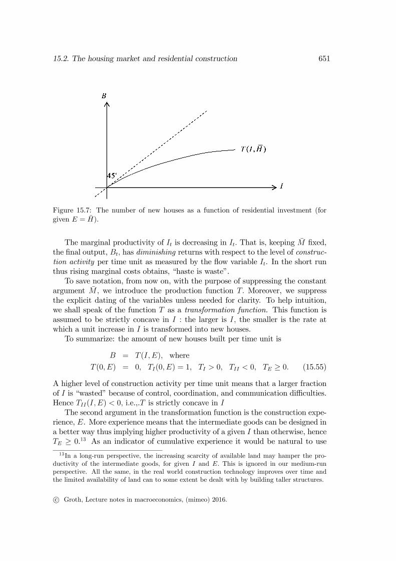
Figure 15.7: The number of new houses as a function of residential investment (forgiven E = H).

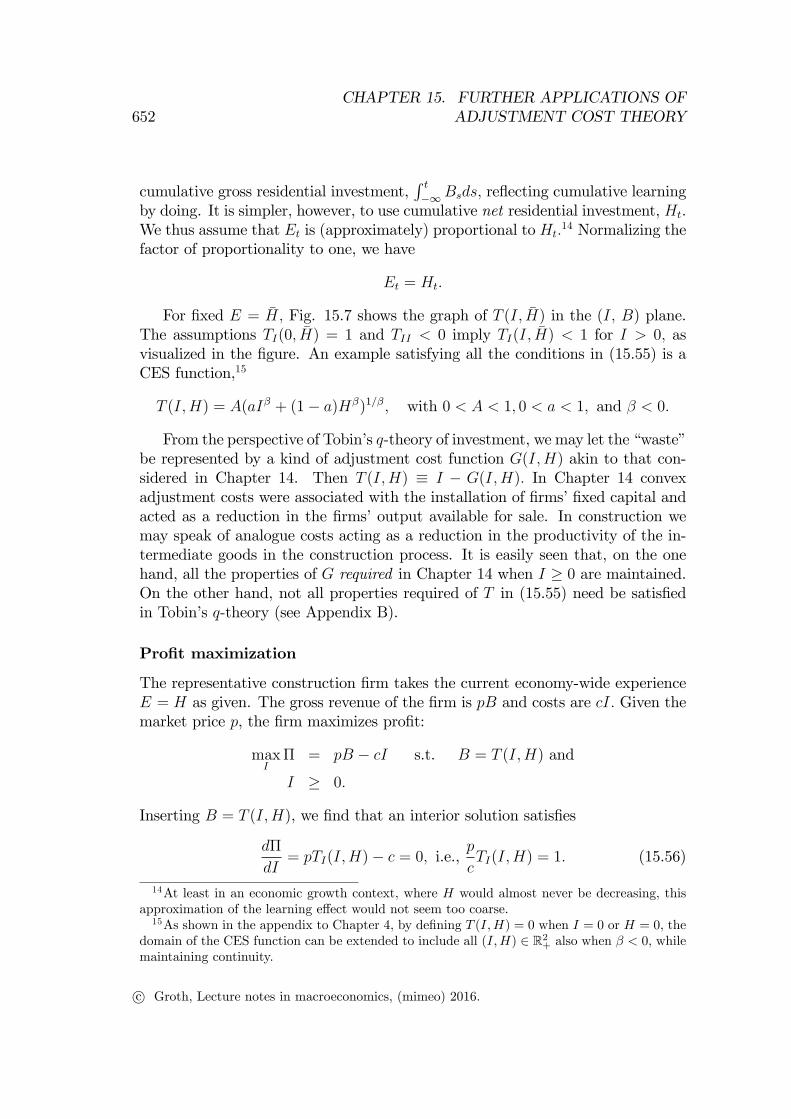
The marginal productivity of It is decreasing in It. That is, keeping M fixed,the final output, Bt, has diminishing returns with respect to the level of construc-tion activity per time unit as measured by the flow variable It. In the short runthus rising marginal costs obtains, “haste is waste”.To save notation, from now on, with the purpose of suppressing the constant

argument M, we introduce the production function T. Moreover, we suppressthe explicit dating of the variables unless needed for clarity. To help intuition,we shall speak of the function T as a transformation function. This function isassumed to be strictly concave in I : the larger is I, the smaller is the rate atwhich a unit increase in I is transformed into new houses.To summarize: the amount of new houses built per time unit is

B = T (I, E), where

T (0, E) = 0, TI(0, E) = 1, TI > 0, TII < 0, TE ≥ 0. (15.55)

A higher level of construction activity per time unit means that a larger fractionof I is “wasted”because of control, coordination, and communication diffi culties.Hence TII(I, E) < 0, i.e.,.T is strictly concave in IThe second argument in the transformation function is the construction expe-

rience, E. More experience means that the intermediate goods can be designed ina better way thus implying higher productivity of a given I than otherwise, henceTE ≥ 0.13 As an indicator of cumulative experience it would be natural to use

13In a long-run perspective, the increasing scarcity of available land may hamper the pro-ductivity of the intermediate goods, for given I and E. This is ignored in our medium-runperspective. All the same, in the real world construction technology improves over time andthe limited availability of land can to some extent be dealt with by building taller structures.




cumulative gross residential investment,∫ t−∞Bsds, reflecting cumulative learning

by doing. It is simpler, however, to use cumulative net residential investment, Ht.We thus assume that Et is (approximately) proportional to Ht.

14 Normalizing thefactor of proportionality to one, we have

Et = Ht.

For fixed E = H, Fig. 15.7 shows the graph of T (I, H) in the (I, B) plane.The assumptions TI(0, H) = 1 and TII < 0 imply TI(I, H) < 1 for I > 0, asvisualized in the figure. An example satisfying all the conditions in (15.55) is aCES function,15

T (I,H) = A(aIβ + (1− a)Hβ)1/β, with 0 < A < 1, 0 < a < 1, and β < 0.

From the perspective of Tobin’s q-theory of investment, we may let the “waste”be represented by a kind of adjustment cost function G(I,H) akin to that con-sidered in Chapter 14. Then T (I,H) ≡ I − G(I,H). In Chapter 14 convexadjustment costs were associated with the installation of firms’fixed capital andacted as a reduction in the firms’output available for sale. In construction wemay speak of analogue costs acting as a reduction in the productivity of the in-termediate goods in the construction process. It is easily seen that, on the onehand, all the properties of G required in Chapter 14 when I ≥ 0 are maintained.On the other hand, not all properties required of T in (15.55) need be satisfiedin Tobin’s q-theory (see Appendix B).

Profit maximization

The representative construction firm takes the current economy-wide experienceE = H as given. The gross revenue of the firm is pB and costs are cI. Given themarket price p, the firm maximizes profit:

maxI

Π = pB − cI s.t. B = T (I,H) and

I ≥ 0.

Inserting B = T (I,H), we find that an interior solution satisfies

dΠ

dI= pTI(I,H)− c = 0, i.e.,

p

cTI(I,H) = 1. (15.56)

14At least in an economic growth context, where H would almost never be decreasing, thisapproximation of the learning effect would not seem too coarse.15As shown in the appendix to Chapter 4, by defining T (I,H) = 0 when I = 0 or H = 0, the

domain of the CES function can be extended to include all (I,H) ∈ R2+ also when β < 0, whilemaintaining continuity.



In view of TI(I,H) < 1 for I > 0, the latter equation has a solution I > 0only if p > c. For p ≤ c, we get the corner solution I = 0. Naturally, when thecurrent market price of houses is below marginal construction cost (which equalsc/(TI(I,H) ≥ c), no new houses will be built. This is a desired property of themodel. On the other hand, when p > c, the construction firm will supply newhouses up to the point where the rising marginal cost equals the current houseprice, p.16

A precise determination of optimal I is obtained the following way. For p > c,the first-order condition (15.56) defines construction activity, I, as an implicitfunction of p/c and H :

I = M(pc,H), where M(1, H) = 0. (15.57)

By implicit differentiation with respect to p/c in (15.56), we find

Mp/c =∂I

∂(p/c)=

−1

(p/c)2TII(I,H)> 0,

where the argument I can be written as in (15.57).

Special case

From now on we assume the transformation function T is homogeneous of degreeone. Thus, B = T (I/H, 1)H. Then, by Euler’s theorem, TI(I,H) is homogeneousof degree 0. So, with explicit timing of the time-dependent variables, (15.56) canbe written

p

cTI

(I

H, 1

)= 1.

This first-order condition defines It/Ht as an implicit function of pt/c :

I

H= m

(pc

), where m(1) = 0. (15.58)

By implicit differentiation with respect to p/c in the first-order condition we find

m′ =−1

(p/c)2TII (I/H, 1)> 0,

where I/H = m(p/c) can be inserted. A construction activity function m withthis property is shown in Fig. 15.8, where c = 1.

16How to come from the transformation function T (I,H) to the marginal cost schedule isdetailed in Appendix C.




Figure 15.8: Construction activity (relative to the housing stock) as a function of themarket price of houses (c = 1).

With explicit timing of the time-dependent variables, and letting bt denotethe flow of new houses relative to the stock of houses, we now have

bt ≡Bt

Ht

=T (It, Ht)

Ht

= T

(ItHt

, 1

)= T

(m(ptc

), 1)≡ b

(ptc

), (15.59)

where b(1) = T (m (1) , 1) = T (0, 1) = 0, b′ = TIm′ > 0.

Remark. Like Tobin’s q, the house price p is the market value of a produced assetwhose supply changes only slowly. As is the case for firms’fixed capital there arestrictly convex stock adjustment costs, represented by the rising marginal con-struction costs. As a result the stock of houses does not change instantaneously iffor instance p changes. But as shown by the above analysis, the flow variable, res-idential construction, responds to p in a way similar to the way firm’s fixed-capitalinvestment responds to Tobin’s q according to the q theory. Recall that Tobin’sq is defined as the economy-wide ratio V/(pIK), where V is the market value ofthe firms, pI is a price index for investment goods, and K is the stock of physicalcapital. The analogue ratio in the housing sector is V (H)/(pI ·H) ≡ p ·H/(pI ·H)= p/c, in view of pI = c. A higher p/c results in more construction activity. �

15.2.3 Equilibrium dynamics under perfect foresight

To determine the evolution over time in H and p, we derive two coupled differ-ential equations in these two variables. When the transformation function T ishomogeneous of degree one, we can in view of 15.59) write (15.54) as

Ht =(b(ptc

)− δ)Ht, (15.60)

where b(1) = 0 and b′ = TIm′ > 0.



Figure 15.9: Phase diagram of aggregate construction activity (c = 1).

Assuming perfect foresight, we have pet = pt for all t. Then we can write (15.53)on the standard form for a first-order differential equation:

pt = [(1− τ r)r + (1− τR)δ + τ p] pt − (1− τR)R(Ht), (15.61)

where R′ < 0.We have hereby obtained a dynamic system inH and p, the coupleddifferential equations (15.60) and (15.61). The corresponding phase diagram isshown in Fig. 15.9.We have H = 0 for b(p/c) = δ > 0. The unique p satisfying this equation is

the steady state value p∗. The H = 0 locus is thus represented by the horizontalline segment p = p∗. The direction of movement for H is positive if p > p∗ andnegative if p < p∗. Since b(1) = 0 and b′ > 0, we have p∗ > c.We have p = 0 for p = (1 − τR)R(H)/ [(1− τ r)r + (1− τR)δ + τ p] . Since

R′(H) < 0, the p = 0 locus has negative slope. The unique steady state value ofH is denoted H∗. To the right of the p = 0 locus, p is rising, and to the left pis falling. The directions of movement of H and p in the different regions of thephase plane are shown in Fig. 15.9.The unique steady state is seen to be a saddle point with housing stock H∗

and housing price p∗. The initial housing stock, H0, is predetermined. Hence,at time t = 0, the economic system must be somewhere on the vertical lineH = H0. The question is whether there can be asset price bubbles in the system.An asset price bubble is present if the market value of the asset for some timesystematically exceeds its fundamental value (the present value of the expectedfuture services or dividends from the asset). Agents might be willing to buy at aprice above the fundamental value if they expect the price will rise further in the




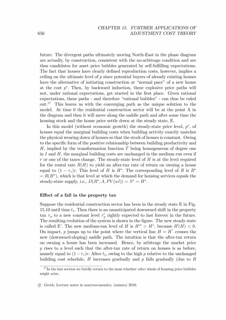
future. The divergent paths ultimately moving North-East in the phase diagramare actually, by construction, consistent with the no-arbitrage condition and arethus candidates for asset price bubbles generated by self-fulfilling expectations.The fact that houses have clearly defined reproduction costs, however, implies aceiling on the ultimate level of p since potential buyers of already existing houseshave the alternative of initiating construction at “normal pace”of a new houseat the cost p∗. Then, by backward induction, these explosive price paths willnot, under rational expectations, get started in the first place. Given rationalexpectations, these paths - and therefore “rational bubbles”- can thus be ruledout.17 This leaves us with the converging path as the unique solution to themodel. At time 0 the residential construction sector will be at the point A inthe diagram and then it will move along the saddle path and after some time thehousing stock and the house price settle down at the steady state, E.In this model (without economic growth) the steady-state price level, p∗, of

houses equal the marginal building costs when building activity exactly matchesthe physical wearing down of houses so that the stock of houses is constant. Owingto the specific form of the positive relationship between building productivity andH, implied by the transformation function T being homogeneous of degree onein I and H, the marginal building costs are unchanged in the medium run even ifr or one of the taxes change. The steady-state level of H is at the level requiredfor the rental rate R(H) to yield an after-tax rate of return on owning a houseequal to (1 − τ r)r. This level of H is H∗. The corresponding level of R is R∗

= R(H∗), which is that level at which the demand for housing services equals thesteady-state supply, i.e., D(R∗, A, PV (wl)) = S∗ = H∗.

Effect of a fall in the property tax

Suppose the residential construction sector has been in the steady state E in Fig.15.10 until time t1. Then there is an unanticipated downward shift in the propertytax τ p to a new constant level τ ′p rightly expected to last forever in the future.The resulting evolution of the system is shown in the figure. The new steady stateis called E’. The new medium-run level of H is H∗′ > H∗, because R′(H) < 0.On impact, p jumps up to the point where the vertical line H = H

∗crosses the

new (downward-sloping) saddle path. The intuition is that the after-tax returnon owning a house has been increased. Hence, by arbitrage the market pricep rises to a level such that the after-tax rate of return on houses is as before,namely equal to (1− τ r)r. After t1, owing to the high p relative to the unchangedbuilding cost schedule, H increases gradually and p falls gradually (due to R

17In the last section we briefly return to the issue whether other kinds of housing price bubblesmight arise.



Figure 15.10: Response to a fall in the property tax (c = 1).

falling with the rising H). This continues until the new steady state is reachedwith unchanged p∗, but higher H.

The dichotomy between the short and medium run

There is a dichotomy between the price and quantity adjustment in the short andmedium run:

1. In the short run, H, hence also the supply of housing services, is given. Therental rate R as well as the house price p immediately shifts up (down) ifthe demand for housing services shifts up (down).

2. In the medium run (i.e., without new disturbances), it isH that adjusts anddoes so gradually. The adjustment of H is in a direction indicated by thesign of the initial price difference, p − p∗, which in turn reflects the initialposition of the demand curve in Fig. 15.6. On the other hand, the houseprice, p, converges towards the cost-determined level, p∗. This price levelis constant as long as technical progress in the production of intermediategoods for construction follows the general trend in the economy.

15.2.4 Discussion

In many countries a part of the housing market is under some kind of rent control.Then there is, of course, rationing on the demand side of the housing market. Itmay still be possible to use the model in a modified version since the part of




the housing market, which is not under regulation and therefore has a marketdetermined price, p, usually includes the new building activity.We have carried out partial equilibrium analysis in a simplified framework.

Possible refinements of the analysis include considering household optimizationwith an explicit distinction between durable consumption (housing demand) andnon-durable consumption and allowing uncertainty and credit market imperfec-tions. Moreover, a general equilibrium approach would take into account thepossible feedbacks on the financial wealth, A, from changes in H and possiblyalso p.18 Allowing economic growth with rising wages in the model would also bepreferable, so that a steady state with a growing housing stock can be considered(a growing housing stock at least in terms of quality-adjusted housing units). Amore complete analysis would also include land prices and ground rent.

The issue of housing bubbles After a decade of sharply rising house prices,the US experienced between 2006 and 2009 a fall in house prices of about 30%(Shiller, ), in Denmark about 20% (Economic Council, Fall 2011). We arguedbriefly that in the present model with rational expectations, housing bubbles canbe ruled out. Let us here go a little more into detail about the concepts involved.The question is whether the large volatility in house prices should be seen as

reflecting the rise and burst of housing bubbles or just volatility of fundamentals.A house price bubble is present if the market price, pt, of houses for some timesystematically exceeds the fundamental value, that is, if pt > pt, where pt is thefundamental value (the present value of the expected future services or dividendsfrom the asset). The latter can be found as the solution to the differential equation(15.61), assuming absence of housing price bubbles (see Appendix D).Our model assumes rational expectations which in the absence of stochastic el-

ements in the model amounts to perfect foresight. What we ruled out by referringto the well-defined reproduction costs of houses was that a rational deterministicasset price bubble could occur in the system. A rational asset price bubble is anasset price bubble that is consistent with the relevant no-arbitrage condition, here(15.53), when agents have model-consistent expectations. If stochastic elementsare added to the model, a rational housing bubble (which would in this case be

18Feedbacks from changes in p are more intricate than one might imagine at first glance.In a representative agent model everybody is an average citizen and owns the house she livesin. Nobody is better off by a rise in house prices. In a model with heterogeneous agents,those who own more houses than they use themselves gain by a rise in house prices. Andthose in the opposite situation lose. Whether and how aggregate consumption is affecteddepends on differences in the marginal propensity to consume and on institutional circumstancesconcerning collaterals in credit markets. In two papers by Case, Quigley, and Shiller (2005,2011) empirical evidence of a positive relationship between consumption and housing wealth inthe US is furnished.


15.3. Literature notes 659

stochastic) can still be ruled out (the argument is similar to the one given for thedeterministic case).Including land and unique building sites with specific amenity values into the

model will, however, make the argument against rational bubbles less compelling(see, e.g., Kocherlakota, 2011). Moreover, there are reasons to believe that inthe real world, expectations are far from always rational. The behavioral financeliterature has suggested alternative theories of speculative bubbles where marketpsychology (herding, fads, etc.) plays a key role. We postpone a more detaileddiscussion of asset price bubbles to Part VI.

15.3 Literature notes

(incomplete)Poterba (1984).Attanasio et al., 2009.Buiter, Housing wealth isn’t wealth, WP, London School of Economics, 20-

07-2008.The question of systematic bias in homebuyer’s expectations in four U.S.

metropolitan areas over the period 2003-2012 is studied in Case, Shiller, andThompson (2012), based on questionnaire surveys. See also Cheng, Raina, andXiong (2012).Campbell and Cocco, 2007.Mayer (2011) surveys theory and empirics about the cyclical movement of

house prices.The phenomenon that fast expansion may reduce effi ciency when managerial

capability is a fixed production factor is known as a Penrose effect, so namedafter a book from 1959 on management by the American economist Edith Pen-rose (1914-1996). Uzawa (1969) explores Penrose’s ideas in different economiccontexts. The construction process is sensitive to managerial capability which isa scarce resource in a construction boom.

15.4 Appendix

A. Complementary inputs

In Section 15.1.2 we claimed, without proof, certain properties of the oil demandfunction and the marginal productivities of capital and labor, respectively, ingeneral equilibrium, given firms’profit maximization subject to a three-factorproduction function with inputs that exhibit direct complementarity. Here, we




use the attributes of the production function F , including (15.2), and the first-order conditions of the representative firm, to derive the claimed signs of thepartial derivatives of the functions M(K, pM), w(K, pM), and MPK(K, pM).First, taking the total derivative w.r.t. K and M in (15.13) gives

FMKdK + FMMdM = dpM .

Hence, ∂M/∂K = −FMK/FMM > 0, and ∂M/∂pM = 1/FMM < 0.Second, taking the total derivative w.r.t. K and pM in (15.12) gives

dw = FLKdK + FLM(MKdK +MpMdpM).

Hence, ∂w/∂K = FLK + FLMMK > 0, and ∂w/∂pM = FLMMpM < 0.Third, ∂MPK/∂pM = FKMMpM < 0, since FKM > 0 and MpM < 0. As to

the sign of ∂MPK/∂K, observe that

∂MPK/∂K = FKK + FKMMK = FKK + FKM(−FMK/FMM)

=1

FMM

(FKKFMM − FKM 2) < 0,

where the inequality follows from FMM < 0, if FKKFMM − FKM 2 > 0. And thelatter inequality does indeed hold. This follows from (15.62) in the lemma below.

Lemma. Let f(x1, x2,x3) be some arbitrary concave C2-function defined on R3+.

Assume fii < 0 for i = 1, 2, 3, and fij > 0, i 6= j. Then, concavity of f impliesthat

fiifjj − fij2 > 0 for i 6= j. (15.62)

Proof. By the general theorem on concave C2-functions (see Math Tools), fsatisfies

f11 ≤ 0, f11f22 − f122 ≥ 0 and

f11(f22f33 − f232)− f12(f21f33 − f23f31) + f13(f21f32 − f22f31) ≤ 0 (15.63)

in the interior of R3+. Combined with the stated assumptions on f , (15.63) implies

(15.62) with i = 2, j = 3. In view of symmetry, the numbering of the argumentsof f is arbitrary. So (15.62) also holds with i = 1, j = 3 as well as i = 1, j = 2. �The lemma applies because F satisfies all the conditions imposed on f in the

lemma. First, the direct complementarity condition fij > 0, i 6= j, is directlyassumed in (15.2). Second, the condition fii < 0 for i = 1, 2, 3 is satisfied byF since, in view of F being neoclassical, the marginal productivities of F arediminishing. Finally, as F in addition to being neoclassical has non-increasingreturns to scale, F is concave.


15.4. Appendix 661

B. The transformation function and the adjustment cost function inTobin’s q-theory

As mentioned in Section 15.2.2 we may formulate the strictly concave transfor-mation function T (I,H) as being equal to I − G(I,H), where the “waste" isrepresented by an adjustment cost function G(I,H) familiar from Chapter 14.Then, on the one hand, all the properties of G required in Chapter 14.1 whenI ≥ 0 are maintained. On the other hand, not all properties required of T in(15.55) need be satisfied in Tobin’s q-theory.As to the first claim, note that when the function T (I,H) ≡ I −G(I,H) has

all the properties stated in (15.55), then the function G must, for (I,H) ∈ R2+,

satisfy:

G(I,H) = I − T (I,H),

G(0, H) = 0− T (0, H) = 0,

GI(I,H) = 1− TI(I,H) ≥ 0, with GI ≥ 0 for I ≥ 0, respectively,

GII(I,H) = −TII(I,H) > 0 for all I ≥ 0,

GH(I,H) = −TH(I,H) ≤ 0,

where the second line is implied by TI(0, H) = 1 and TII < 0. These conditionson G for (I,H) ∈ R2

+ are exactly those required in Chapter 14.1.As to second claim, a requirement on the function T in (15.55) is that TI(0, H) =

1 and TI(I,H) > 0 for all I ≥ 0 at the same time as TII < 0. This requires that0 < TI(I,H) < 1 for all I > 0. For G(I,H) = I − T (I,H) to be consistent withthis, we need that 0 < GI < 1 for all I > 0. So the G function should not be “tooconvex”in I. We would have to impose the condition that limI→∞GII = 0 holdswith “suffi cient”speed of convergence. Whereas for instance

G(I,H) = I − A(aIβ + (1− a)Hβ)1/β, with 0 < A < 1, 0 < a < 1, and β < 0,

will do, a function like G(I/H) = (α/2)I2/H, α > 0, will not do for large I.Nevertheless, the latter function satisfies all conditions required in Tobin’s q-theory.If for some reason one would like to use such a quadratic function to represent

waste in construction, one could relax the in (15.55) required condition TI(I,H) >0 to hold only for I below some upper bound.Finally, we observe that when T (I,H) ≡ I −G(I,H), then, if the function G

is homogeneous of degree k, so is the function T, and vice versa.




Figure 15.11: Marginal costs in house construction (housing stock given).

C. Interpreting construction behavior in a marginal cost perspective(Section 15.2.2)

We may look at the construction activity of the representative construction firmfrom the point of view of increasing marginal costs in the short run. First, let T Cdenote the total costs per time unit of the representative construction firm. Wehave T C = f + T VC, where f is the fixed cost to management and T VC is thetotal variable cost associated with the construction of B (= T (I,H)) new housesper time unit, given the economy-wide stock H. All these costs are measuredin real terms. We have T VC = cI. The input of intermediates, I, required forbuilding B new houses per time unit is an increasing function of B. Indeed, theequation

B = T (I,H), (*)

where TI > 0, defines I as an implicit function of B and H, say I = ϕ(B,H). Byimplicit differentiation in (*) we find

ϕB = ∂I/∂B = 1/TI(ϕ(B,H), H) > 1, when I > 0

So T VC = cI = cϕ(B,H), and short-run marginal cost is

MC(c, B,H) =∂T VC∂B

= cϕB =c

TI(ϕ(B,H), H)> c, when I > 0. (**)

CLAIM(i) The short-run marginal cost, MC, of the representative construction firm isincreasing in B.(ii) The construction sector produces new houses up the point whereMC = p.(iii) The cost of building one new house per time unit is approximately c.


15.4. Appendix 663

Proof. (i) By (**) and (*),

∂MC∂B

=−cTII(ϕ(B,H), H)ϕBTI(ϕ(B,H), H)2

=−cTII(ϕ(B,H), H)

TI(ϕ(B,H), H)3> 0,

since TI > 0 and TII < 0. (ii) Follows from (**) and the first-order condi-tion (15.56) found in the text. (iii) The cost of building ∆B, when B = 0,isMC(c,∆B,H) ≈ [c/TI(0, H)] ·∆B = c∆B = c when ∆B = 1, where we haveused (**). �

That it is profitable to produce new houses up the point where MC = p isillustrated in Fig. 15.11.

D. Solving the no-arbitrage equation for pt in the absence of houseprice bubbles (Section 15.2.4)

By definition, if there are no housing bubbles, the market price of a house equalsits fundamental value, i.e., the present value of expected (possibly imputed) after-tax rental income from owning the house. Denoting the fundamental value pt, wethus have

pt = (1− τR)

∫ ∞t

R(Hs)e−(τp+δ)(s−t)eτRδ(s−t)e−(1−τr)r(s−t)ds, (15.64)

= (1− τR)

∫ ∞t

R(Hs)e−[(1−τr)r+(1−τR)δ+τp](s−t)ds,

where the three discount rates appearing in the first line are, first, τ p + δ, whichreflects the rate of “leakage”from the investment in the house due to the propertytax and wear and tear, second, τRδ, which reflects the tax allowance due to wearand tear, and, finally, (1 − τ r)r, which is the usual opportunity cost discount.In the second row we have done an addition of the three discount rates so as tohave just one discount factor easily comparable to the discount factor appearingbelow.In Section 15.2.4 we claimed that in the absence of housing bubbles, the linear

differential equation, (15.61), implied by the no-arbitrage equation (15.53) underperfect foresight, has a solution pt equal to the fundamental value of the house,i.e., pt = pt. To prove this, we write (15.61) on the standard form for a lineardifferential equation,

pt + apt = −(1− τR)R(Ht), (15.65)

wherea ≡ − [(1− τ r)r + (1− τR)δ + τ p] < 0. (15.66)




The general solution to (15.65) is

pt =

(pt0 − (1− τR)

∫ t

t0

R(Hs)ea(s−t0)ds

)e−a(t−t0).

Multiplying through by ea(t−t0) gives

ptea(t−t0) = pt0 − (1− τR)

∫ t

t0

R(Hs)ea(s−t0)ds.

Rearranging and letting t→∞, we get

pt0 = (1− τR)

∫ ∞t0

R(Hs)ea(s−t0)ds+ lim

t→∞pte

a(t−t0).

Inserting (15.66), replacing t by T and t0 by t, and comparing with (15.64), wesee that

pt = pt + limT→∞

pT e−[(1−τr)r+(1−τR)δ+τp](T−t).

The first term on the right-hand side is the fundamental value of the house attime t. The second term on the right-hand side thus amounts to the differencebetween the market price of the house and its fundamental value. By definition,this difference represents a bubble. In the absence of the bubble, the marketprice, pt, therefore coincides with the fundamental value.On the other hand, we see that a bubble being present requires that

limT→∞

pT e−[(1−τr)r+(1−τR)δ+τp](T−t) > 0.

In turn, this requires that the house price is explosive in the sense of ultimatelygrowing at a rate not less than (1 − τ r)r + (1 − τR)δ + τ p. The candidate for abubbly path ultimately moving North-East portrayed in Fig. 15.9 in fact has thisproperty. Indeed, by (15.61), for such a path we have

pt/pt = [(1− τ r)r + (1− τR)δ + τ p]−(1−τR)R(Ht)/pt → (1−τ r)r+(1−τR)δ+τ p for t→∞,

since pt →∞ and R′(Ht) < 0.

15.5 Exercises

(15.61)


15.2 The housing market and residential con- struction

Documents

Transcript of 15.2 The housing market and residential con- struction