Introduction to Statistical Learning Theory

MIT 15.097 Course NotesCynthia Rudin

Credit: A large part of this lecture was taken from an introduction to learningtheory of Bousquet, Boucheron, Lugosi

Now we are going to study, in a probabilistic framework, the properties of learningalgorithms. At the beginning of the semester, I told you that it was importantfor our models to be “simple” in order to be able to generalize, or learn fromdata. I didn’t really say that precisely before, but in this lecture I will.

Generalization = Data + Knowledge

Finite data cannot replace knowledge. Knowledge allows you to choose a simplerset of models.

Perhaps surprisingly, there is no one universal right way to measure simplicity orcomplexity of a set of models - simplicity is not an absolute notion. But we’ll giveseveral precise ways to measure this. And we’ll precisely show how our abilityto learn depends on the simplicity of the models. So we’ll make concrete (viaproof) this philosophical argument that learning somehow needs simplicity.

In classical statistics, the number of parameters in the model is the usual mea-sure of complexity. Here we’ll use other complexity measures, namely the GrowthFunction and VC dimension (which is a beautiful combinatorial quantity), cov-ering number (the one I usually use), and Rademacher average.

Assumptions

Training and test data are drawn iid from the same distribution. If there’s norelationship between training and test, there’s no way to learn of course. (That’slike trying to predict rain in Africa next week using data about horse-kicks inthe Prussian war) so we have to make some assumption.

1

Each learning algorithm encodes specific knowledge (or a specific assumption,perhaps about what the optimal classifier must look like) and works best whenthis assumption is satisfied by the problem to which it is applied.

Notation

Input space X , output space Y = {−1, 1}, unknown distribution D on X × Y .We observe m iid pairs {(xi, yi)}mi=1 drawn iid from D. The goal is to constructa function f : X → Y that predicts y from x.

We would like the true risk to be as small as possible, where the true risk is:

Rtrue(f) := P(X,Y ) D(f(X) = Y ) = E∼ (X,Y )∼D[1f(X)=Y ].

Did you recognize this nice thing that comes from the definition of expecta-tion and probability? We can flip freely between notation for probability andexpectation.

PZ D(Z = blah) =∑

1[outcome=blah]PZ D(Z = outcome) = E∼ ∼ Z∼D1[Z=blah].outcomes

We introduce the regression function

η(x) = E(X,Y ) D(Y |X = x)∼

and the target function (or Bayes classifier)

t(x) = sign η(x).

Think of the distribution D, which looks sort of like this:

6 6

2

Here’s the function η:

Now take the sign of it:

And that’s t:

3

The target function achieves the minimum risk over all possible measurable func-tions:

Rtrue(t) = inf Rtrue(f).f

We denote the value Rtrue(t) by R∗, called the Bayes Risk.

Our goal is to identify this function t but since D is unknown, we cannot evaluatet at any x.

The empirical risk that we can measure is:

memp 1

R (f) = ym

∑1[f(xi)= i].

i=1

Algorithm

Most of the calculations don’t depend on a specific algorithm, but you can thinkof using regularized empirical risk minimization.

f ∈ argmin Remp(f) + C‖f‖2m f∈F

for some norm. The regularization term will control the complexity of the modelto prevent overfitting. The class of functions that we’re working with is F .

6

4

Bounds

Remember, we can compute fm and Remp(fm), but we cannot compute thingslike Rtrue(fm).

The algorithm chooses fm from the class of functions F . Let us call the bestfunction in the class f ∗, so that

Rtrue(f ∗) = inf Rtrue(f).f∈F

Then, I would like to know how far Rtrue(fm) is from R∗. How bad is the functionwe chose, compared to the best one, the Bayes Risk?

Rtrue(fm)−R∗ = [Rtrue(f ∗)−R∗] + [Rtrue(fm)−Rtrue(f ∗)]

= Approximation Error + Estimation Error .

The Approximation Error measures how well functions in F can approach thetarget (it would be zero if t ∈ F). The Estimation Error is a random quantity(it depends on data) and measures how close is fm to the best possible choice inF .

Draw Approximation Error and Estimation Error

Figuring out the Approximation Error is usually difficult because it requiresknowledge about the target, that is, you need to know something about thedistribution D. In Statistical Learning Theory, generally there is no assumptionmade about the target (such as its belonging to some class). This is probably themain reason why this theory is so important - it does not require any knowledgeof the distribution D.

Also, even if the empirical risk converges to the Bayes risk as m gets large (thealgorithm is consistent), it turns out that the convergence can be arbitrarily slowif there is no assumption made about the regularity of the target. On the otherhand, the rate of convergence of the Estimation Error can be computed withoutany such assumption. We’ll focus on the Estimation Error for this class.

We would really like to understand how bad the true risk of our algorithm’soutput, Rtrue(fm), could possibly be. We want this to be as small as possible of

5

course. We’ll consider another way to look at Rtrue(fm):

Rtrue(fm) = Remp(f truem) + [R (fm)−Remp(fm)], (1)

where remember we can measure Remp(fm).

We could upper bound the term Rtrue(fm) − Remp(fm), to make something likethis:

Rtrue(fm) ≤ Remp(fm) + Stuff(m,F).

The “Stuff” will get more interesting as this lecture continues.

A Bound for One Function f

Let’s define the loss g corresponding to a function f . The loss at point (x, y) is:

g(x) = 1f(x)=y.

Given F , define the loss class, which contains all of the loss functions comingfrom F .

G = {g : (x, y)→ 1f(x)=y : f ∈ F}.So g doesn’t look at predictions f , instead it looks at whether the predictionswere correct. Notice that F contains functions with range in {−1, 1} while Gcontains functions with range {0, 1}.

There’s a bijection between F and G. You can go from an f to its g byg(x, y) = 1f(x)=y. You can go from a g to its f by saying that if g(x, y) = 1then set f(x) = −y, otherwise set f(x) = y. We’ll use the g notation wheneverwe’re bounding the difference between an empirical average and its mean becausethe notation is slightly simpler.

Define this notation:

P trueg = E(X,Y )∼D[g(X, Y )] (true risk again)

m

P emp 1g =

∑g(Xi, Yi) (empirical risk again)

mi=1

so that we have another way to write the true risk and empirical risk directlyin terms of the loss. P emp is called the empirical measure associated to the

6

6

6

6

training sample. It just computes the average of a function at the trainingpoints. Remember, we are interested in the difference between the true risk andempirical risk, same thing as in the right side of (1), which we’re going to upperbound:

P truegm − P empgm. (2)

(gm is the loss version of fm.)

Hoeffding’s Inequality

For convenience we’ll define Zi = (Xi, Yi) and Z = (X, Y ), and probabilities willbe taken with respect to Z1 ∼ D, ..., Zm ∼ D which we’ll write Z ∼ Dm.

Let’s rewrite the quantity we’re interested in, for a general g this time:∑m1P trueg − P empg = EZ∼Dm[g(Z)]− g(Zi).

mi=1

It’s a difference between an empirical mean and its expectation. By the law oflarge numbers we know asymptotically that the mean converges to the expecta-tion in probability. So with probability 1, with respect to Z ∼ Dm,

m1

lim∑

g(Zi) = EZm→∞m

∼Dm[g(Z)].i=1

So with enough data, the empirical risk is a good approximation to its true risk.

There’s a quantitative version of the law of large numbers when variables arebounded:

Theorem 1 (Hoeffding). Let Z1...Zm be m iid random variables, and h is abounded function, h(Z) ∈ [a, b]. Then for all ε > 0 we have:[∣∣∣ ∑m1 2

PZ∼Dm ∣ 2mε∣ h(Zi)− EZ∼Dm[h(Z)]

∣∣≥ ε

]∣ ≤ 2 expm

(∣∣ − .(b− a)2

i=1

)The probability that the empirical average and expectation are far from eachother is small. Let us rewrite the formula to better understand its consequences.

7

Let the right hand side be δ, so (2mε2

δ = 2 exp −(b− a)2

).

Then if I solve for ε, I get: √log 2

ε = (b− a) δ

2m

So Hoeffding’s inequality, applied to the function g becomes:

P emp true log 2δ

Z Dm

|P g − P g| ≥ (b− a)

√ ≤ δ.∼2m

There’s a technique called “inversion” that we’ll use a lot.

Inversion

Using inversion, we get that with probability at least 1− δ:

2

|P emp logg − P trueg| ≤ (b− a)

√δ .

2m

The expression above is “2-sided” in that there’s an absolute value on the left.This considers whether P empg is larger than P trueg or smaller than it. There’salso 1-sided versions of Hoeffding’s inequality where we look at deviations in onedirection or the[other, for instance here is a 1-sided version of Hoeffding’s:

m1 2mε2

PZ Dm EZ Dm[h(Z)]∼ ∼ −m

∑h(Zi) ≥ ε

]≤ exp

(− .

(b=1

− a)2i

)If we again set the right side to δ and solve for ε, and invert, we get that withprobability at least 1− δ,

m1 log 1

EZ∼Dm[h(Z)]−m

∑h(Zi) (b a) δ .

2mi=1

≤ −

√Here is the inverted one applied to g: with probabilit√ y at least 1− δ,

log 1

P trueg − P empg ≤ (b− a) δ .2m

8

Moving the empirical term to the right, we have that with probability at least1− δ,

1

P trueg ≤ P emp logg + (b− a)

√δ .

2m

Remember that g is the loss, so g(Z) = 1f(X)=Y and that way we have an upperbound for the true risk, which we want to be small.

This expression seems very nice, but guess what? It doesn’t apply when f (i.e.,g) comes from any reasonable learning algorithm!

Why not?

Limitations

The result above says that for each fixed function g ∈ G, there is a set S of“good” samples z1, ..., zm, for which

true emp

√log 1

P g − P g ≤ (1− 0) δ

2m

and this set of samples has measure PZ∼Dm[Z ∈ S] ≥ 1− δ. However, these setsmay be different for different functions g. In other words, for the sample S weactually observe, there’s no telling how many of the functions in G will actuallysatisfy this inequality!

This figure might help you understand. Each point on the x-axis is a differentfunction. The curve marked Rtrue(f) is the true risk, which is a constant for eachf since it involves the whole distribution (and not a sample).

6

9

If you give me a sample and a function f , I can calculate Remp(f) for that sample,which gives me a dot on the plot. So, for each sample we get a different curve onthe figure. For each f , Hoeffding’s inequality makes sure that most of the time,the Remp(f) curves lie within a small distance of Rtrue(f), though we don’t knowwhich ones. In other words, for an observed sample, only some of the functionsin F will satisfy the inequality, not all of them.

But remember, our algorithms choose fm knowing the data. They generally tryto minimize the regularized Remp(f). Consider drawing a sample S, which cor-responds to a curve on the figure. Our algorithm could (on purpose) meanderalong that curve until it chooses a fm that gives a small value of Remp. This valuecould be very far from Rtrue(fm). This could definitely happen, and if there aremore f ’s to choose from (if the function class is larger), then this happens moreeasily - uh oh! In other words, if F is large enough, one can find, somewherealong the axis, a function f for which the difference between the two curvesRemp(f) and Rtrue(f) will be very large.

10

We don’t want this to happen!

Uniform Bounds

We really need to make sure our algorithm doesn’t do this - otherwise it willnever generalize. That’s why we’re going to look at uniform deviations in orderto upper bound (1) or (2):

Rtrue(fm)−Remp(fm) ≤ sup(Rtrue(f)f

−Remp(f))∈F

where we look at the worst deviation over all functions in the class.

Let us construct a first uniform bound, using Hoeffding’s inequality and theunion bound. Define:

Cj = {z1, ..., zm : P truegj − P empgj ≥ ε}.

This set contains all the “bad” samples, those for which the bound fails forfunction gj. From Hoeffding’s Inequality, for each j,

PZ Dm[Z ∈ Cj] ≤ δ.∼

Consider two functions g1 and g2. Say we want to measure how many samplesare “bad” for either one of these functions or the other. We’re going to use theunion bound to do this, which says:

P[C1 ∪ C2] ≤ P[C1] + P[C2] ≤ 2δ,

the probability that we hit a bad sample for either g1 or g2 is≤

prob to hit a bad sample for C1 + prob to hit a bad sample for C2.

More generally, the union bound is:

N

P[C1 ∪ ... ∪ CN ] ≤∑

P[Cj]j=1

≤ Nδ

11

So this is a bound on the probability that our chosen sample will be bad for anyof the functions g1, ..., gN . So we get:

PZ Dm[∃g ∈ {g1, ..., gN : P trueg P empg ε]∼ ∑N } − ≥

≤ PZ m[∼D P truegj P empgj ε]j=1

− ≥

N

≤∑

exp(−2mε2) Where did this come from?j=1

= N exp(−2mε2).

If we define a new δ so we can invert:

δ := N exp(−2mε2)

and solve for ε, we get: √logN + log 1

ε = δ .2m

Plugging that in and inverting, we find that with probability at least 1− δ,

1

∀g ∈ {g1, ..., gN} : P trueg − emp logN + logP g ≤

√δ .

2m

Changing g’s back to f ’s, we’ve proved the following:

Theorem. (Hoeffding + Union Bound)For F = {f1...fN}, for all δ > 0 with probability at least 1− δ,

∀f ∈ F , Rtrue logN + log 1

(f) ≤ Remp(f) +

√δ .

2m

Just to recap the reason why this bound is better than the last one, if we knowour algorithm only picks functions from a finite function class F , we now have abound that can be applied to fm, even though it depends on the data.

Note the main difference with plain Hoeffding’s inequality is the extra logN termon the right hand side. This term is the one saying we want N bounds to holdsimultaneously.

12

Estimation Error

Let’s say we’re doing empirical risk minimization, that is, fm is the minimizer ofthe empirical risk Remp.

We can use the theorem above (combined with (1)) to get an upper bound onthe Estimation Error. Start with this:

Rtrue(fm) = Rtrue(fm)−Rtrue(f ∗) +Rtrue(f ∗)

Then we’ll use the fact that Remp(f ∗)−Remp(fm) ≥ 0. Why is that?

We’ll add that to the expression above:

Rtrue(f ) ≤ [Remp(f ∗)−Remp truem (fm)] +R (fm)−Rtrue(f ∗) +Rtrue(f ∗)

= Remp(f ∗)−Rtrue(f ∗)−Remp(fm) +Rtrue(fm) +Rtrue(f ∗)

≤ |Rtrue(f ∗)−Remp(f ∗)|+ |Rtrue(fm)−Remp(fm)|+Rtrue(f ∗)

≤ 2 sup Rtrue(f) Remp(f) +Rtrue(f ∗).f| − |

∈F

We could use a 2-sided version of the theorem (with an extra factor of 2 some-where) that with probability 1− δ, that first term is bounded by the square rootterm in the theorem. Specifically, we know that with probability 1− δ:

2

Rtrue logN + log(fm) ≤ 2

√δ +Rtrue(f ∗).

2m

Actually, if you think about it, both terms in the right hand side depend on thesize of the class F . If this size increases, the first term will increase, and thesecond term will decrease. Why?

Summary and Perspective

• Generalization requires knowledge (like restricting f to lie in a restrictedclass F).

• The error bounds are valid with respect to the repeated sampling of trainingsets.

13

• For a fixed function f , for most of the samples,

Rtrue(f)−Remp(f) ≈ 1/√m.

• For most of the samples if the function class if finite, |F| = N ,

sup[Rtrue(g) logg

−Remp(g)] ≈∈G

√N/m.

The extra term is because we choose fm in a way that changes with thedata.

• We have the Hoeffding + Union Bound Theorem above, which bounds theworst difference between empirical risk and true risk among functions in theclass.

There are several things that could be improved. For instance Hoeffding’s in-equality only uses the boundedness of the functions, not their variance, which issomething we won’t deal with here. The supremum over F of Rtrue(f)−Remp(f)is not necessarily what the algorithm would choose, so the upper bound couldbe loose. The union bound is in general loose, because it is as bad as if all thefj(Z)’s are independent.

Infinite Case: VC Dimension

Here we’ll show how to extend the previous results to the case where the classF is infinite.

We’ll start with a simple refinement of the union bound that allows to extendthe previous results to the (countably) infinite case.Recall that by Hoeffding’s inequality for a single function g, for each δ > 0, wherepossibly we could choose δ depending on g, which we write δ(g), we have:

1

PZ Dm

log δ(g)

P trueg empg∼ − P ≥

√2m

≤ δ(g).

Hence if we have a countable

set

G, the union bound gives:

log 1

P δZ Dm

∃g ∈ G (g): P trueg g∼ − P emp ≥

√2m

≤∑ δ(g).g∈G

14

If we choose the δ(g)’s so that they add up to a constant total value δ, that is,δ(g) = δ p(g) where

∑g p(g) = 1, then the right hand side is just δ and we get∈G

the following with inversion: with probability at least 1− δ,

log 1

∀ ∈ G true ≤ emp

√+ log 1

p(g) δg , P g P g + .

2m

If G is finite with size N , and we take a uniform p(g) = 1 , we get the logN termN

as before.

General Case

When the set G is uncountable, the previous approach doesn’t work because p(g)is a density, so it’s 0 for a given g and the bound will be vacuous. We’ll switchback to the original class F rather than the loss class for now. The general ideais to look at the function class’s behavior on the sample. Given z1, ..., zm, weconsider

Fz1,...,zm = {f(z1), ..., f(zm) : f ∈ F}.Fz1,...,zm is the set of ways the data z1, ..., zm are classified by functions from F .Since the functions f can only take two values, this set will always be finite, nomatter how big F is.

Definition (Growth Function) The growth function is the maximum numberof ways into which m points can be classified by the function class:

S (m) = supF(z1,...,zm)

|Fz1,...,zm|.

Intuition for Growth Function and Example of Halfplanes

We defined the growth function in terms of the initial class F but we cando the same with the loss class G since there’s a 1-1 mapping, so we’ll getS (m) = S (m).G F

This growth function can be used as a measure of the ‘size’ of a class of functionsas demonstrated by the following result:

15

Theorem-GrowthFunction (Vapnik-Chervonenkis) For any δ > 0, withprobability at least 1− δ with respect to a random draw of the data,

logS (2m) + log 4

∀f ∈ F Rtrue(f) ≤ Remp(f) + 2

√2

F δ

m

(proof soon).

This bound shows nicely that simplicity implies generalization. The simpler thefunction class, the better the guarantee that Rtrue will be small. In the finitecase where |F| = N (we have N possible classifiers), we have S (m)F ≤ N (atworst we use up all the classifiers when we’re computing the growth function). Sothis bound is always better than the one we had before (except for the constants).

But we need to figure out how to compute S (m). We’ll do that using VCFdimension.

VC dimension

Since f ∈ {−1, 1}, it is clear that S (m)F ≤ 2m.

If S (m) = 2m there is a data set of size m points such that F can generate anyFclassification on these points (we say F shatters the set).

The VC dimension of a class F is the size of the largest set that it can shatter.

Definition. (VC dimension) The VC dimension of a class F is the largest msuch that

S (m) = 2m.F

What is the VC dimension of halfplanes in 2 dimensions?

Can you guess the VC dimension of halfplanes in d dimensions?

In the example, the number of parameters needed to define the half space in Rd

is the number of dimensions, d. So a natural question to ask is whether the VCdimension is related to the number of parameters of the function class. In other

16

words, VC dimension is supposed to measure complexity of a function class -does it just basically measure the number of parameters?

Is the VC dimension always close to the number of parameters?

So how can VC dimension help us compute the growth function? Well, if a classof functions has VC dim h, then we know that we can shatter m examples whenm ≤ h, and in that case, S (m) = 2m. If m > h, then we know we can’t shatterFthe points, so S (m) < 2m otherwise.F

This doesn’t seem very helpful perhaps, but actually an intriguing phenomenonoccurs for m ≥ h, shown below.

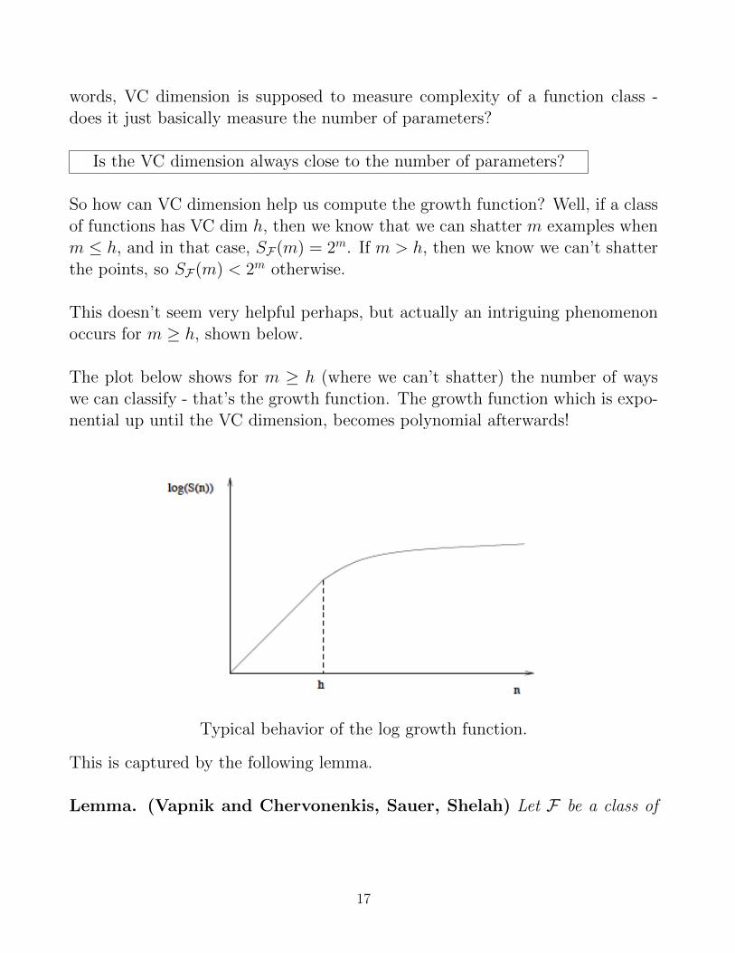
The plot below shows for m ≥ h (where we can’t shatter) the number of wayswe can classify - that’s the growth function. The growth function which is expo-nential up until the VC dimension, becomes polynomial afterwards!

Typical behavior of the log growth function.

This is captured by the following lemma.

Lemma. (Vapnik and Chervonenkis, Sauer, Shelah) Let F be a class of

17

functions with finite VC dimension h. Then for all m ∈ N,

h

S (m)F ≤∑i=0

(m

i

)Intuition

and for all m ≥ h

S (m)F ≤

Using this lemma for m h along with Theo

(em.

h

)h≥ rem-GrowthFunction, we get:

Theorem VC-Bound. If F has VC dim h, and for m ≥ h, with prob. at least1− δ,

∀f ∈ F Rtrue h log 2em + log 4

(f) ≤ Remp(f) + 2

√2 h δ .

m

What is important to remember from this result is that the difference betweenthe true and empirical risk is at most of order√

h logm.

m

Before we used VC dim, the bound was infinite, i.e., vacuous!

Recap

Why is Theorem VC-Bound important? It shows that limiting the complexity ofthe class of functions leads to better generalization. An interpretation of VC dimand growth functions is that they measure the “effective” size of the class, that is,the size of the projection of the class onto finite samples. This measure doesn’tjust count the number of functions in the class, but depends on the geometryof the class, that is, the projections onto the possible samples. Also since theVC dimension is finite, our bound shows that the empirical risk will convergeuniformly over the class F to the true risk.

Back to Margins

How is it that SVM’s limit the complexity? Well, the choice of kernel controlsthe complexity. But also the margin itself controls complexity. There is a set of

18

linear classifiers called “gap-tolerant classifiers” that I won’t define precisely (itgets complicated) that require a margin of at least ∆ between points of the twodifferent classes. The points are also forced to live inside a sphere of diameter D.So the class of functions is fairly limited, since they not only need to separatethe points with a margin of ∆, but also we aren’t allowed to move the pointsoutside of the sphere.

“Theorem” VC-Margin. (Vapnik) For data in Rd, the VC dimension h

of (linear) gap-tolerant classifiers classifiers with gap ∆ belong to a sphere ofdiameter D, is bounded by the inequality:

h ≤ min

(⌈D2

12

⌉, d

)+ .

∆

So the VC dimension (of the set of functions that separate points with somemargin) is less than 1/margin. If we have a large margin, we necessarily have asmall VC-dimension.

What does this say about halfspaces in Rd?(Think about the VC dimension example we did earlier.)

Symmetrization

We’ll do the proof of Theorem-GrowthFunction. The key ingredient is the sym-metrization lemma. We’ll use what’s called a “ghost sample” which is an extra(virtual) data set Z1

′ , ..., Zm′ . Denote P ′emp the corresponding empirical measure.

(Lemma-Symmetrization) For any t > 0, such that mt2 ≥ 2,

PZ∼Dm

[sup(P true

g− P emp)g ≥ t

∈G

]≤ 2PZ∼Dm,Z′∼Dm

[sup(P ′emp

g− P emp)g ≥ t/2

∈G

].

That is, if we can bound the difference between the behavior on one sample ver-sus another, it gives us a bound on the behavior of a sample with respect to thetrue risk.

Proof. Let gm be the function achieving the supremum in the lhs term, whichdepends on Z1, ...Zm. Think about the event that: (P true P emp)gm t (the− ≥

19

sample’s loss is far from the true loss) and (P true − P ′emp)gm < t/2 (the ghostsample’s loss is close to the true loss). If this event were true, it sort of means thatthings didn’t generalize well for Z1, ..., Zm but that they did generalize well forZ1′ , ..., Zm

′ . If we can show that this event happens rarely, then the ghost samplecan help us. Again, the event that we want to happen rarely is (P true−P emp)gm ≥t and (P true − P ′emp)gm < t/2.

1(P true−P emp)gm≥t1(P true−P ′emp)gm<t/2

= 1(P true−P emp)g ≥t and (P true empm −P ′ )gm<t/2

= 1(P true−P emp)gm≥t and (P ′emp−P true)gm>−t/2

≤ 1(P true−P emp+P ′emp−P true)g >t−t/2=t/2 = 1(−P emp empm +P ′ )gm>t/2.

The inequality came from the fact that the event on the second last line ((P true−P emp)gm ≥ t and (P ′emp − P true)gm > −t/2) implies the event on the last line((P true − P emp + P ′emp − P true)gm > t− t/2), so the event on the last line couldhappen more often.Taking expectations with respect to the second sample, and using the trick tochange expectation into probability,

1 P [(P true − P ′emp(P true P emp)gm t Z′ Dm )gm < t/2]− ≥ ∼

≤ PZ′ Dm[(P ′emp − P emp)gm > t/2]. (3)∼

Do you remember Chebyshev’s Inequality? It says P[|X − EX| ≥ t] ≤ VarX/t2.We’ll apply it now, to that second term on the left, inverted:

4VPZ′ Dm[(P true − P ′emp argm

)gm ≥ t/2]∼ ≤ .mt2

I hope you’ll believe me when I say that any random variable that has range[0, 1] has variance less than or equal to 1/4. Hence,

1PZ′ Dm[(P true − P ′emp)gm ≥ t/2]∼ ≤ .

mt2

Inverting back, so that it looks like the second term on the left of (3) again:

1PZ′ Dm[(P true − P ′emp)gm < t/2] ≥ 1∼ − .

mt2

Multiplying both sides by 1(P true−P emp( )gm≥t I get back to the left of (3):

11 1−

)≤ 1 P [(P true

emp)g t′emp

(P true P emp)gm t (P true P Z′ Dmm

− P )gm < t/2]− ≥mt2

− ≥ ∼

≤ PZ′∼Dm[(P ′emp − P emp)gm > t/2] from (3).

20

Taking the expectation with respect to the first sample, the term

EZ∼Dm1 true emp(P true−P emp)gm≥t becomes PZ∼Dm[(P − P )gm ≥ t].

And now we get:

P [(P true emp 1Z Dm −P )gm ≥ t]

(1−

)≤ PZ′ DmZ Dm[(P ′emp

∼mt2

∼ ∼ −P emp)gm > t/2]

P true 1[(P −P emp)g ≥ t] ≤

( )P [(P ′emp−P emp

Z∼Dm m Z′∼DmZ∼Dm )g1− m > t/2].1

mt2

Only one more step, which uses our assumption mt2 ≥ 2.

mt2 ≥ 21 1

mt2≤

21 1 1

1−mt2

≥ 1− =( 2 21

1− 1mt2

)≤ 2

Plug:

PZ Dm[(P true − P emp)g empm ≥ t] ≤ 2PZ′ DmZ Dm[([P ′emp − P )g >∼ ∼ m t/2]∼

≤ 2P empZ Dm,Z′ Dm sup(P ′ − P emp)g > t/2∼ ∼

g∈G

].

We have an upper bound by changing the strict inequality “>” to a “≥.” Thenthe result is the same as the statement of the lemma. �

Remember, we’re still in the middle of proving Theorem-GrowthFunction. Thesymmetrization is just a step in that proof. This symmetrization lemma allows usto replace the expectation P trueg by an empirical average over the ghost sample.As a result, the proof will only depends on the projection of the class G on thedouble sample

GZ1...Zm,Z1′ ...Zm

′ ,

which contains finitely many different vectors. In other words, an element of thisset is just the vector [g(x1), ..., g(xm)], and there are finitely many possibilitiesfor vectors like this. So we can use the union bound that we used for the finite

21

case. The other ingredient that we need to prove Theorem-GrowthFunction isthis one:

P 2

[P empg − P ′empg ≥ t] ≤ 2e−mt /2Z∼DmZ′∼Dm . (4)

This one comes itself from a mix of Hoeffding’s with the union bound:

P [P empg − P ′empZ∼DmZ′∼Dm g ≥ t]

= P emp true trueZ DmZ′ Dm[P g − P g + P g − P ′empg t∼ ∼ ≥ ]

≤ PZ∼Dm[P empg − P trueg t/2] + P true empZ′ [∼Dm P g P ′ g t/2]

≤ e−2m(t/2)2 + e−2m(t/2)2≥ − ≥

= 2e−mt2/2.

We just have to put the pieces together now:

P trueZ∼Dm[sup(P

g− P emp)g ≥ t]

∈G

≤ 2PZ DmZ′ Dm[sup(P ′emp∼

g− P emp)g ≥ t/2] Lemma-Symmetrization∼

∈G

= 2P emp empZ∼DmZ′∼Dm[ sup (P ′ P )g t/2] (restrict to data)∑ g∈GZ ,...,Zm,Z′ ,...,Z1 1 m

′

− ≥

≤ 2 PZ DmZ′ Dm[(P ′emp∼ ∼

g

− P emp)g ≥ t/2] (union bound)∈GZ ,...,Z1 m,Z′ ,...,Z1 m

′

≤ 2∑

2e−m(t/2)2/2

g∈GZ ,...,Z1 m,Z′ ,...,Z1 m′

2

= 4e−mt /8

g∈GZ ,...,Z1

∑1

m,Z1′ ,...,Zm

′

= 4S (2m) e−mt2/8.G

And using inversion,

P true emp mt2/8Z∼Dm[sup(P )

g− P g ≤ t] ≥ 1− 4S (2m) e− .G

∈G

Letting δ = 4S (2m) e−mt2/8, solving for t yields:G

t =

√8 4S (2m)

logG

m δ

22

Plug:

PZ∼Dm

S + 4

sup( true

g− P emp log (2m) log

P )g ≤ 2∈G

√2

G δ

m

≥ 1− δ.

So, with probability at least 1− δ,

∀g ∈ G (P true − P emp)g ≤ 2

√logS (2m) + log 4

2G δ .

m

That’s the result of Theorem-GrowthFunction. �

Other kinds of capacity measures

One important aspect of VC dimension is that it doesn’t depend on D, so itis a distribution independent quantity. The growth function is also distributionindependent. That’s nice in some ways, because it allows us to get bounds thatdon’t depend on the problem at hand: the same bound holds for any distribu-tion. Although this may seem like an advantage, it could also be a drawbacksince, as a result, the bound may be loose for most distributions.

It turns out there are several different quantities that are distribution dependent,which we can use in generalization bounds.

VC-entropy

One quantity is called the (annealed) VC entropy. Recall the notation |Gz1,...,zm|which is the number of ways we can correctly/incorrectly classify z1, ..., zm.

VC-entropyG(m) := logEZ Dm[ ]∼ |GZ1,...,Zm| .

If the VC-entropy is large, it means that a lot of the time, there are a lot ofdifferent ways to classify m data points. So the capacity of the set of functionsis somehow large. There’s a bound for the VC-entropy that’s very similar to theone for Theorem-GrowthFunction (which I won’t go into here).

How does the VC-entropy relate to the Growth Function?

23

Covering Number

Another quantity is called the covering number. Covering numbers can be de-fined in several different ways, but we’ll just define one of them. Let’s start byendowing the function class G with the following (random) metric:

m1

dm(g, g′) =∑

1[g(Zm i)=g′(Zi)],

i=1

the fraction of times they disagree on the (random) sample.

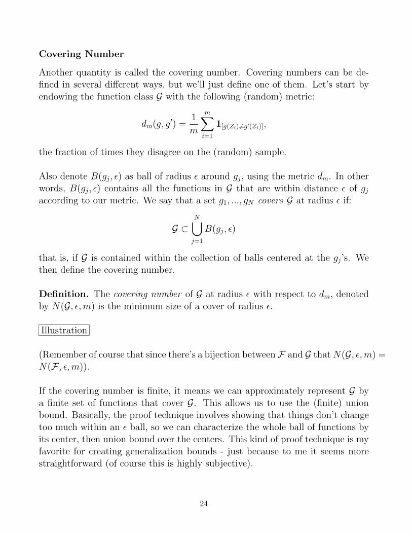
Also denote B(gj, ε) as ball of radius ε around gj, using the metric dm. In otherwords, B(gj, ε) contains all the functions in G that are within distance ε of gjaccording to our metric. We say that a set g1, ..., gN covers G at radius ε if:

N

G ⊂j

⋃B(gj, ε)

=1

that is, if G is contained within the collection of balls centered at the gj’s. Wethen define the covering number.

Definition. The covering number of G at radius ε with respect to dm, denotedby N(G, ε,m) is the minimum size of a cover of radius ε.

Illustration

(Remember of course that since there’s a bijection between F and G thatN(G, ε,m) =N(F , ε,m)).

If the covering number is finite, it means we can approximately represent G bya finite set of functions that cover G. This allows us to use the (finite) unionbound. Basically, the proof technique involves showing that things don’t changetoo much within an ε ball, so we can characterize the whole ball of functions byits center, then union bound over the centers. This kind of proof technique is myfavorite for creating generalization bounds - just because to me it seems morestraightforward (of course this is highly subjective).

6

24

A typical result (stated without proof) is:

Theorem-Covering. For any t > 0,

P [∃f ∈ F : Rtrue(f) ≥ Remp(f) + t] ≤ 8E [N(F , t,m)]e−mt2/128

Z∼Dm Z∼Dm .

We can relate the covering number to the VC dimension.

Lemma (Haussler). Let F be a class of VC dimension h. Then for all ε > 0,all m, and any sample,

N(F , ε,m) ≤ Ch(4e)hεh.

(where C is a constant). One thing about this result is that the upper bounddoes not depend on the sample size m. Probably it is a loose upper bound, butit’s nice to be able to get this independent of m!

Rademacher Averages

Another way to measure complexity is to see how well functions from the classF can classify random noise. So if I arbitrarily start flipping the labels, how wellcan functions from my class fit those arbitrary labels. If the functions from F canfit those arbitrary labels really well, then F must have high complexity. That’sthe intuition behind the Rademacher complexity measure that we’re going tointroduce.

I’m going to introduce some notation,

m1

Rmg :=∑

σig(Zi)m

i=1

where the σi’s are independent {+1,−1}-valued random variables with proba-bility 1/2 of taking either value. You can think of them as random coin flips.Denote Eσ the expectation taken with respect to the σi’s.

Definition. (Rademacher Averages) For a class G of functions, the Rademacheraverage is defined as:

R(G) := Eσ,Z supRmg.g∈G

25

In other words, for each set of flips of the coin, you consider them as labels foryour data, and find a function from G that matches them the best. If you canmatch a lot of random coin flips really well using functions from G, then G hashigh complexity.

Here’s a bound involving Rademacher averages:

Theorem-RademacherBound. With probability at least 1− δ,

log 2

∀g ∈ G, Rtrue(g) ≤ Remp(g) + 2R(G) +

√δ .

2m

The proof of this requires a powerful tool called a concentration inequality. Ac-tually, Hoeffding’s inequality is a concentration inequality, so you’ve seen one al-ready. Concentration inequalities say that as m increases, the empirical averageis concentrated around the expectation. McDiarmid’s concentration inequalityis my favorite, and it generalizes Hoeffding’s in that applies to functions thatdepend on m iid random variables:

Theorem. (McDiarmid’s Inequality) Assume for all i = 1, ...,m

sup |F (z1, ..., zi, ..., zm)− F (z1, ..., zi′, ..., zm)

z1,...,zm,zi′

| ≤ c

then for all ε > 0,

2ε2P[|F − E[F ]| ≥ ε] ≤ 2 exp

(−mc2

).

This is a Hoeffding-like inequality that holds for any function of m variables, aslong as replacing one of those variables by another one won’t allow the functionto change too much.

Proof of Theorem-RademacherBound

We’ll follow two steps:

• concentration to relate supg (P trueg∈G − P empg) to its expectation,

26

• symmetrization to relate the expectation to the Rademacher average.

We want to use McDiarmid’s inequality on supg (P trueg−P empg), so we’ll need∈Gto show that if we modify one training example, it doesn’t change too much.Denote P emp,i as the empirical measure obtained by replacing zi by zi

′ of thesample. The following holds:

| sup(P trueg )g

− P empg − sup(P trueg∈G g

− P emp,ig)| ≤ sup∈G g

|P emp,ig − P empg|. (5)∈G

This isn’t too hard to check. For instance, let’s say that the first term is largerthan the second so we can remove the absolute value. Then say g∗ achievessupg (P trueg∈G − P empg). Then

sup(P trueg − P empg)− sup(P trueg g∈G g

− P emp,i )g ∈G

= (P trueg∗ − P empg∗)− sup(P truegg

− P emp,ig)∈G

≤ (P trueg∗ − P empg∗)− (P trueg∗ P emp,ig∗)

= P emp,ig∗ − P empg∗ ≤ sup(P emp,i

−g

g− P empg)

∈G

And if the second term is larger than the first, we do an identical calculation.So (5) holds.

P emp,ig−P emp mg is a difference of two averages, since remember P empg is 1m i=1 g(Zi)

and P emp,ig is the same thing except that the ith term got replaced with

∑g(Zi

′).

1 1|P emp,ig − P empg| = |g(Zi′)

m− g(Zi)| ≤

m

where we used that g ∈ {0, 1} for the last inequality.

This means from (5) that we have

| sup(P truegg

− P empg)− sup(P trueg P emp,i 1g) , (6)

∈G g− | ≤

m∈G

the function F = supg (P trueg − P empg) can’t change more than 1 when we∈G m

fiddle with one of the Zi’s. This means we can directly apply McDiarmid’sinequality to it with c = 1 .m

2ε2PZ Dm[| sup(P trueg−P empg)−E true

Z Dm[sup(P g−P empg)]| ≥ ε] ≤ 2 exp

(−

).∼

g∼

g m 1∈G ∈G m2

27

That’s the first part of the proof (the concentration part).

Now for symmetrization, which we’ll use to prove that the expected differencebetween the true and empirical risks is bounded by twice the Rademacher aver-age.

Lemma.

EZ Dm sup[P trueg∼g

− P empg] ≤ 2Eσ,Z supRmg = 2R(∈G g

G)∈G

To prove it, we introduce a ghost sample and it’s corresponding measure P ′emp.We’re going to use that E true

Z P emp∼Dm

′ g = P g in the second line below.

EZ Dm sup[P trueg∼g

− P empg]∈G

= E sup[E [P ′empg − P empZ∼Dm Z′

g∼Dm g]]

∈G

≤ E emp empZ DmZ′ Dm sup[P ′ g − P g] (uses Jensen’s Inequality, sup is convex)∼ ∼

g∈G

= EZ,Z′

[m

1sup

∑(g(Zi

′)− g(Zi))g m∈G i=1

]

= Eσ,Z,Z′

[sup

∑m1σi(g(Zi

′)− g(Zi))

]Why?

≤ Eσ,Z

[ g m∈G i=1

m m1 1

sup∑

σig(Z ′)m i sup

∈G

]+ Eσ,Z

g

[g m

i=1 ∈G

∑σig(Zi)

i=1

−

]= 2Eσ,Z supRmg.

g∈G

The last step uses that σig(Zi) and −σig(Zi) have the same distribution. �

Let’s put the two parts of the proof of Theorem-RademacherBound together.The first part said:

2

P [| sup(P trueg−P empg)−E [sup(P true emp 2εZ∼Dm Z

g∼Dm g

g−P g)]| ≥ ε] ≤ 2 exp

(−

1/m∈G ∈G

).

The second part said:

EZ∼Dm sup[P trueg ]g

− P empg ≤ 2Eσ,Z supRmg = 2R( )∈G g

G∈G

28

Let’s fiddle with the first part. First, let

2

:= 2 exp

(2ε log 2

δ − so that ε = δ

1/m

) √2m

So the first part looks like

logPZ Dm

∣∣∣ 2∣sup(P trueg∼ − P empg)− E true emp δZ∼Dm

g

[sup(P g )] δ.g

− P g

]∣ √∣∣∣ ≥ 2m∈G ∈G

≤Using inversion, with probability at least 1− δ,∣∣∣ log 2∣sup(P trueg

g− P empg)− EZ D

[sup P emp

m (P trueg − g)∼∈G g

]∣≤

∈G

√δ .

2m

I can remove the absolute value and the left hand side only gets

∣∣∣smaller. Then,

sup(P trueg − P empg) ≤ E[sup(P trueg − P empg)]

]+

√log 2

δZ Dm .

g∼

∈G g 2m∈G

Using the second part,

log 2

sup(P trueg − P empg) ≤ 2R( )g

G +∈G

√δ .

2m

Writing it all together, with probability at least 1− δ, for all g ∈ G,

P trueg ≤ P empg + 2R(G) +

√log 2

δ ,2m

and that’s the statement of Theorem-RademacherBound.�

Relating the Rademacher Complexity of the Loss Class

and the Initial Class

Theorem RademacherBound is nice, but it only applies to the class G, and wealso care about class , so we need to relate the Rademacher average of toF G

29

that of class F . We do this as follows, using the fact that σi and Yiσi have thesame distribution.

R(G) = Eσ,Z

[m

1sup

∑σi1[f(Xi)=Yi]

g m∈G i=1

]

= Eσ,Z

[m

1sup

∑ 1σi (1− Yif(Xi))

g m 2∈G i=1

]Why?

m1 1 1

= Eσ,Z sup σiYif(Xi) = ( ). Why?2

[g m 2

R∈G

∑i=1

]F

Ok so we’ve related the two classes’ Rademacher averages. So, with probabilityat least 1− δ,

∀f ∈ F , Rtruef ≤ Remp log 2

f +R(F) +

√δ .

2m

Computing the Rademacher Averages

Let’s assess the difficulty of actually computing Rademacher averages. Starthere:

m1 1 1R(F) = Eσ,Z

[sup

∑σif(Xi)

2 2 f m∈F i=1

]1

= + Eσ,Z2

[m

1 1 σisup

− f(Xi)

[f m

∑=1

−2∈F i

]m

1 1 1− σ− E∑

if(Xi)= σ,Z inf

2 f∈F m 2i=1

]m

1 1= − Eσ,Z

[inf

∑1f(Xi)=σi

]. (1/2 comes through the inf)

2 f∈F mi=1

Look closely at that last expression. The thing on the inside says to find theempirical risk minimizer, where the labels are the σi’s. This expression showsthat computing R(F) is not any harder than computing the expected empirical

6

6

30

risk minimizer over random labels. So we could design a hypothetical procedure,where we generate the σi’s randomly, and minimize the empirical error in G withrespect to the labels σi. (Of course we technically also have to do this over thepossible Xi’s, but there are some ways to get around this that I won’t go intohere.)

It’s also true thath log em

R(F) ≤ 2

√h

m

So we could technically use the Rademacher complexity bound to get anotherVC-bound.So we’re done! We showed formally that limiting the complexity leads to bettergeneralization. We gave several complexity measures for a set of models (GrowthFunction, VC-dimension, VC-entropy, Covering Number, Rademacher averages).

31

MIT OpenCourseWarehttp://ocw.mit.edu

15.097 Prediction: Machine Learning and StatisticsSpring 2012

For information about citing these materials or our Terms of Use, visit: http://ocw.mit.edu/terms.