15. Basic Index Number Theory
33
370 15. Basic Index Number Theory A. Introduction The answer to the question what is the Mean of a given set of magnitudes cannot in general be found, unless there is given also the object for the sake of which a mean value is required. There are as many kinds of average as there are purposes; and we may almost say, in the matter of prices as many purposes as writers. Hence much vain controversy between persons who are literally at cross purposes. (F.Y. Edgeworth, 1888, p. 347) 15.1 The number of physically distinct goods and unique types of services that consumers can purchase is in the millions. On the business or pro- duction side of the economy, there are even more products that are actively traded. The reason is that firms not only produce products for final consump- tion, they also produce exports and intermediate products that are demanded by other producers. Firms collectively also use millions of imported goods and services, thousands of different types of labor services, and hundreds of thousands of spe- cific types of capital. If we further distinguish physical products by their geographic location or by the season or time of day that they are produced or consumed, then there are billions of products that are traded within each year in any advanced economy. For many purposes, it is necessary to summarize this vast amount of price and quantity information into a much smaller set of numbers. The question that this chapter addresses is the fol- lowing: How exactly should the microeconomic in- formation involving possibly millions of prices and quantities be aggregated into a smaller number of price and quantity variables? This is the basic in- dex number problem. 15.2 It is possible to pose the index number problem in the context of microeconomic theory; that is, given that we wish to implement some eco- nomic model based on producer or consumer the- ory, what is the best method for constructing a set of aggregates for the model? However, when con- structing aggregate prices or quantities, other points of view (that do not rely on economics) are possible. Some of these alternative points of view will be considered in this chapter and the next chapter. Economic approaches will be pursued in Chapters 17 and 18. 15.3 The index number problem can be framed as the problem of decomposing the value of a well- defined set of transactions in a period of time into an aggregate price multiplied by an aggregate quantity term. It turns out that this approach to the index number problem does not lead to any useful solutions. Therefore, in Section B, the problem of decomposing a value ratio pertaining to two peri- ods of time into a component that measures the overall change in prices between the two periods (this is the price index) multiplied by a term that measures the overall change in quantities between the two periods (this is the quantity index) is con- sidered. The simplest price index is a fixed-basket index. In this index, fixed amounts of the n quanti- ties in the value aggregate are chosen, and then this fixed basket of quantities at the prices of period 0 and period 1 are calculated. The fixed-basket price index is simply the ratio of these two values, where the prices vary but the quantities are held fixed. Two natural choices for the fixed basket are the quantities transacted in the base period, period 0, or the quantities transacted in the current period, period 1. These two choices lead to the Laspeyres (1871) and Paasche (1874) price indices, respec- tively. 15.4 Unfortunately, the Paasche and Laspeyres measures of aggregate price change can differ, sometimes substantially. Thus, Section C considers taking an average of these two indices to come up with a single measure of price change. Section C.1 argues that the best average to take is the geomet- ric mean, which is Irving Fisher’s (1922) ideal price index. In Section C.2, instead of averaging the Paasche and Laspeyres measures of price change, taking an average of the two baskets is considered. This fixed-basket approach to index number theory leads to a price index advocated by Walsh (1901, 1921a). However, other fixed-basket
Transcript of 15. Basic Index Number Theory
370
15. Basic Index Number Theory
A. Introduction
The answer to the question what is the Mean of a given set of magnitudes cannot in general be found, unless there is given also the object for the sake of which a mean value is required. There are as many kinds of average as there are purposes; and we may almost say, in the matter of prices as many purposes as writers. Hence much vain controversy between persons who are literally at cross purposes. (F.Y. Edgeworth, 1888, p. 347)
15.1 The number of physically distinct goods and unique types of services that consumers can purchase is in the millions. On the business or pro-duction side of the economy, there are even more products that are actively traded. The reason is that firms not only produce products for final consump-tion, they also produce exports and intermediate products that are demanded by other producers. Firms collectively also use millions of imported goods and services, thousands of different types of labor services, and hundreds of thousands of spe-cific types of capital. If we further distinguish physical products by their geographic location or by the season or time of day that they are produced or consumed, then there are billions of products that are traded within each year in any advanced economy. For many purposes, it is necessary to summarize this vast amount of price and quantity information into a much smaller set of numbers. The question that this chapter addresses is the fol-lowing: How exactly should the microeconomic in-formation involving possibly millions of prices and quantities be aggregated into a smaller number of price and quantity variables? This is the basic in-dex number problem.
15.2 It is possible to pose the index number problem in the context of microeconomic theory; that is, given that we wish to implement some eco-nomic model based on producer or consumer the-ory, what is the best method for constructing a set of aggregates for the model? However, when con-structing aggregate prices or quantities, other
points of view (that do not rely on economics) are possible. Some of these alternative points of view will be considered in this chapter and the next chapter. Economic approaches will be pursued in Chapters 17 and 18.
15.3 The index number problem can be framed as the problem of decomposing the value of a well-defined set of transactions in a period of time into an aggregate price multiplied by an aggregate quantity term. It turns out that this approach to the index number problem does not lead to any useful solutions. Therefore, in Section B, the problem of decomposing a value ratio pertaining to two peri-ods of time into a component that measures the overall change in prices between the two periods (this is the price index) multiplied by a term that measures the overall change in quantities between the two periods (this is the quantity index) is con-sidered. The simplest price index is a fixed-basket index. In this index, fixed amounts of the n quanti-ties in the value aggregate are chosen, and then this fixed basket of quantities at the prices of period 0 and period 1 are calculated. The fixed-basket price index is simply the ratio of these two values, where the prices vary but the quantities are held fixed. Two natural choices for the fixed basket are the quantities transacted in the base period, period 0, or the quantities transacted in the current period, period 1. These two choices lead to the Laspeyres (1871) and Paasche (1874) price indices, respec-tively.
15.4 Unfortunately, the Paasche and Laspeyres measures of aggregate price change can differ, sometimes substantially. Thus, Section C considers taking an average of these two indices to come up with a single measure of price change. Section C.1 argues that the best average to take is the geomet-ric mean, which is Irving Fisher’s (1922) ideal price index. In Section C.2, instead of averaging the Paasche and Laspeyres measures of price change, taking an average of the two baskets is considered. This fixed-basket approach to index number theory leads to a price index advocated by Walsh (1901, 1921a). However, other fixed-basket
15. Basic Index Number Theory
371
approaches are also possible. Instead of choosing the basket of period 0 or 1 (or an average of these two baskets), it is possible to choose a basket that pertains to an entirely different period, say, period b. In fact, it is typical statistical agency practice to pick a basket that pertains to an entire year (or even two years) of transactions in a year before pe-riod 0, which is usually a month. Indices of this type, where the weight reference period differs from the price reference period, were originally proposed by Joseph Lowe (1823), and in Section D indices of this type will be studied. They will also be evaluated from the axiomatic perspective in Chapter 16 and from the economic perspective in Chapter 17.1
15.5 In Section E, another approach to the de-termination of the functional form or the formula for the price index is considered. This approach, devised by the French economist Divisia (1926), is based on the assumption that price and quantity data are available as continuous functions of time. The theory of differentiation is used to decompose the rate of change of a continuous time value ag-gregate into two components that reflect aggregate price and quantity change. Although Divisia’s ap-proach offers some insights,2 it does not offer much guidance to statistical agencies in terms of leading to a definite choice of index number formula.
15.6 In Section F, the advantages and disadvan-tages of using a fixed-base period in the bilateral index number comparison are considered versus always comparing the current period with the pre-vious period, which is called the chain system. In the chain system, a link is an index number com-parison of one period with the previous period. These links are multiplied to make comparisons over many periods.
1Indices of this type will not appear in Chapter 19, where
most of the index number formulas exhibited in Chapters 15–18 will be illustrated using an artificial data set. How-ever, indices where the weight reference period differs from the price reference period will be illustrated numeri-cally in Chapter 22, where the problem of seasonal prod-ucts will be discussed.
2In particular, it can be used to justify the chain system of index numbers, which will be discussed in Section E.2.
B. Decomposition of Value Aggregates into Price and Quantity Components
B.1 Decomposition of value aggregates and the product test
15.7 A price index is a measure or function that summarizes the change in the prices of many products from one situation 0 (a time period or place) to another situation 1. More specifically, for most practical purposes, a price index can be re-garded as a weighted mean of the change in the relative prices of the products under consideration in the two situations. To determine a price index, it is necessary to know
(i) Which products or items to include in the index,
(ii) How to determine the item prices, (iii) Which transactions that involve these items to
include in the index, (iv) How to determine the weights and from
which sources these weights should be drawn, and
(v) Which formula or mean should be used to av-erage the selected item relative prices.
All the above price index definition questions ex-cept the last can be answered by appealing to the definition of the value aggregate to which the price index refers. A value aggregate V for a given collection of items and transactions is computed as
(15.1) 1
n
i ii
V p q=
= ∑ ,
where pi represents the price of the ith item in na-tional currency units, qi represents the correspond-ing quantity transacted in the time period under consideration, and the subscript i identifies the ith elementary item in the group of n items that make up the chosen value aggregate V. Included in this definition of a value aggregate is the specification of the group of included products (which items to include) and of the economic agents engaging in transactions involving those products (which transactions to include), as well as the valuation and time of recording principles motivating the behavior of the economic agents undertaking the transactions (determination of prices). The in-cluded elementary items, their valuation (the pi),

Producer Price Index Manual
372
the eligibility of the transactions, and the item weights (the qi) are all within the domain of defini-tion of the value aggregate. The precise determina-tion of the pi and qi was discussed in more detail in Chapter 5 and other chapters.3 15.8 The value aggregate V defined by equa-tion (15.1) referred to a certain set of transactions pertaining to a single (unspecified) time period. Now, consider the same value aggregate for two places or time periods, periods 0 and 1. For the sake of definiteness, period 0 is called the base pe-riod and period 1 is called the current period. As-sume that observations on the base-period price and quantity vectors, p0 ≡ [p1
0,…,pn0] and q0 ≡
[q10,…,qn
0], respectively, have been collected.4 The value aggregates in the two periods are de-fined in the obvious way as
(15.2) 0 0 1 10 1; .
1 1
n n
i i i i
i i
V p q V p q= =
≡ ≡∑ ∑
15.9 In the previous paragraph, a price index was defined as a function or measure that summa-rizes the change in the prices of the n products in the value aggregate from situation 0 to situation 1. In this paragraph, a price index P(p0,p1,q0,q1) along with the corresponding quantity index (or volume index) Q(p0,p1,q0,q1) is defined as two functions of the 4n variables p0,p1,q0,q1 (these variables de-scribe the prices and quantities pertaining to the value aggregate for periods 0 and 1), where these two functions satisfy the following equation:5
(15.3) 1 0 0 1 0 1 ( ) V / V P p , p ,q ,q = 0 1 0 1( ) Q p , p ,q ,q× .
3Ralph Turvey and others (1989) have noted that some
values may be difficult to decompose into unambiguous price and quantity components. Some examples of values difficult to decompose are bank charges, gambling expendi-tures, and life insurance payments.
4Note that it is assumed that there are no new or disap-pearing products in the value aggregates. Approaches to the “new goods problem” and the problem of accounting for quality change are discussed in Chapters 7, 8, and 21.
5The first person to suggest that the price and quantity in-dices should be jointly determined to satisfy equation (15.3) was Irving Fisher (1911, p. 418). Frisch (1930, p. 399) called equation (15.3) the product test.
If there is only one item in the value aggregate, then the price index P should collapse to the single-price ratio p1
1/p10, and the quantity index Q
should collapse to the single-quantity ratio q11/q1
0. In the case of many items, the price index P is to be interpreted as some sort of weighted average of the individual price ratios, p1
1/p10,…, pn
1/pn0.
15.10 Thus, the first approach to index number theory can be regarded as the problem of decom-posing the change in a value aggregate, V1/V0, into the product of a part that is due to price change, P(p0,p1,q0,q1), and a part that is due to quantity change, Q(p0,p1,q0,q1). This approach to the de-termination of the price index is the approach taken in the national accounts, where a price index is used to deflate a value ratio to obtain an estimate of quantity change. Thus, in this approach to index number theory, the primary use for the price index is as a deflator. Note that once the functional form for the price index P(p0,p1,q0,q1) is known, then the corresponding quantity or volume index Q(p0,p1,q0,q1) is completely determined by P; that is, by rearranging equation (15.3):
(15.4) ( )0 1 0 1 1 0 ( )Q p , p ,q ,q V /V= 0 1 0 1( )/ P p , p ,q ,q .
Conversely, if the functional form for the quantity index Q(p0,p1,q0,q1) is known, then the correspond-ing price index P(p0,p1,q0,q1) is completely deter-mined by Q. Thus, using this deflation approach to index number theory, separate theories for the de-termination of the price and quantity indices are not required: if either P or Q is determined, then the other function is implicitly determined by the product test, equation (15.4). 15.11 In the next subsection, two concrete choices for the price index P(p0,p1,q0,q1) are con-sidered, and the corresponding quantity indices Q(p0,p1,q0,q1) that result from using equation (15.4) are also calculated. These are the two choices used most frequently by national income accountants.
B.2 Laspeyres and Paasche indices
15.12 One of the simplest approaches determin-ing the price index formula was described in great detail by Joseph Lowe (1823). His approach to
15. Basic Index Number Theory
373
measuring the price change between periods 0 and 1 was to specify an approximate representative product basket,6 which is a quantity vector q ≡ [q1,…,qn] that is representative of purchases made during the two periods under consideration, and then to calculate the level of prices in period 1 relative to period 0 as the ratio of the period 1 cost
of the basket, 1
1
n
i ii
p q=∑ , to the period 0 cost of the
basket, 0
1
n
i ii
p q=∑ . This fixed-basket approach to the
determination of the price index leaves open the following question: How exactly is the fixed-basket vector q to be chosen?
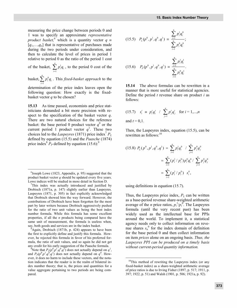
15.13 As time passed, economists and price stat-isticians demanded a bit more precision with re-spect to the specification of the basket vector q. There are two natural choices for the reference basket: the base period 0 product vector q0 or the current period 1 product vector q1. These two choices led to the Laspeyres (1871) price index7 PL defined by equation (15.5) and the Paasche (1874) price index8 PP defined by equation (15.6):9
6Joseph Lowe (1823, Appendix, p. 95) suggested that the
product basket vector q should be updated every five years. Lowe indices will be studied in more detail in Section D.
7This index was actually introduced and justified by Drobisch (1871a, p. 147) slightly earlier than Laspeyres. Laspeyres (1871, p. 305) in fact explicitly acknowledged that Drobisch showed him the way forward. However, the contributions of Drobisch have been forgotten for the most part by later writers because Drobisch aggressively pushed for the ratio of two unit values as being the best index number formula. While this formula has some excellent properties, if all the n products being compared have the same unit of measurement, the formula is useless when, say, both goods and services are in the index basket.
8Again, Drobisch (1871b, p. 424) appears to have been the first to explicitly define and justify this formula. How-ever, he rejected this formula in favor of his preferred for-mula, the ratio of unit values, and so again he did not get any credit for his early suggestion of the Paasche formula.
9Note that PL(p0,p1,q0,q1) does not actually depend on q1, and PP(p0,p1,q0,q1) does not actually depend on q0. How-ever, it does no harm to include these vectors, and the nota-tion indicates that the reader is in the realm of bilateral in-dex number theory; that is, the prices and quantities for a value aggregate pertaining to two periods are being com-pared.
(15.5)
n1 0
0 1 0 1 1n
0 0
1
( ) ;i i
iL
i ii
p qP p , p ,q ,q
p q
=
=
≡∑
∑
(15.6)
n1 1
0 1 0 1 1n
0 1
1
( ) .i i
iP
i ii
p qP p , p ,q ,q
p q
=
=
≡∑
∑
15.14 The above formulas can be rewritten in a manner that is more useful for statistical agencies. Define the period t revenue share on product i as follows:
(15.7) 1
/n
t t t t ti i i j j
js p q p q
=
≡ ∑ for i = 1,...,n
and t = 0,1. Then, the Laspeyres index, equation (15.5), can be rewritten as follows:10
(15.8) 0 1 0 1 1 0 0 0
1 1( , , , ) /
n n
L i i j ji j
P p p q q p q p q= =
= ∑ ∑
1 0 0 0 0 0
1 1
1 0 0
1
( / ) /
( / ) ,
n n
i i i i j ji j
n
i i ii
p p p q p q
p p s
= =
=
=
=
∑ ∑
∑ using definitions in equation (15.7). Thus, the Laspeyres price index, PL can be written as a base-period revenue share-weighted arithmetic average of the n price ratios, pi
1/pi0. The Laspeyres
formula (until the very recent past) has been widely used as the intellectual base for PPIs around the world. To implement it, a statistical agency needs only to collect information on reve-nue shares sn
0 for the index domain of definition for the base period 0 and then collect information on item prices alone on an ongoing basis. Thus, the Laspeyres PPI can be produced on a timely basis without current-period quantity information.
10This method of rewriting the Laspeyres index (or any fixed-basket index) as a share-weighted arithmetic average of price ratios is due to Irving Fisher (1897, p. 517; 1911, p. 397; 1922, p. 51) and Walsh (1901, p. 506; 1921a, p. 92).

Producer Price Index Manual
374
15.15 The Paasche index can also be written in revenue share and price ratio form as follows:11
(15.9) 0 1 0 1 0 1 1 1
1 1
( , , , ) 1n n
P i i j ji j
P p p q q p q p q= =
=
∑ ∑
( )
( )
( )
0 1 1 1 1 1
1 1
11 0 1
1
111 0 1
1
1
1
,
n n
i i i i j ji j
n
i i ii
n
i i ii
p p p q p q
p p s
p p s
= =
−
=
−−
=
=
=
=
∑ ∑
∑
∑
using definitions in equation (15.7). Thus, the Paasche price index PP can be written as a period 1 (or current-period) revenue share-weighted harmonic average of the n item price ra-tios pi
1/pi0.12 The lack of information on current-
period quantities prevents statistical agencies from producing Paasche indices on a timely basis. 15.16 The quantity index that corresponds to the Laspeyres price index using the product test, equa-tion (15.3), is the Paasche quantity index; that is, if P in equation (15.4) is replaced by PL defined by equation (15.5), then the following quantity index is obtained:
(15.10)
1 1
0 1 0 1 1
1 0
1
( ) .
n
i ii
P n
i ii
p qQ p , p ,q ,q
p q
=
=
≡∑
∑
Note that QP is the value of the period 1 quantity
vector valued at the period 1 prices, 1 1
1
n
i ii
p q=∑ , di-
vided by the (hypothetical) value of the period 0 quantity vector valued at the period 1 prices,
1 0
1
n
i ii
p q=∑ . Thus, the period 0 and 1 quantity vectors
11This method of rewriting the Paasche index (or any
fixed-basket index) as a share-weighted harmonic average of the price ratios is due to Walsh (1901, p. 511; 1921a, p. 93) and Irving Fisher (1911, pp. 397–98).
12Note that the derivation in equation (15.9) shows how harmonic averages arise in index number theory in a very natural way.
are valued at the same set of prices, the current-period prices, p1. 15.17 The quantity index that corresponds to the Paasche price index using the product test, equa-tion (15.3), is the Laspeyres quantity index; that is, if P in equation (15.4) is replaced by PP defined by equation (15.6), then the following quantity index is obtained:
(15.11)
0 1
0 1 0 1 1
0 0
1
( ) .
n
i ii
L n
i ii
p qQ p , p ,q ,q
p q
=
=
≡∑
∑
Note that QL is the (hypothetical) value of the pe-riod 1 quantity vector valued at the period 0 prices,
0 1
1
n
i ii
p q=∑ , divided by the value of the period 0
quantity vector valued at the period 0 prices, 0 0
1
n
i ii
p q=∑ . Thus, the period 0 and 1 quantity vectors
are valued at the same set of prices, the base-period prices, p0. 15.18 The problem with the Laspeyres and Paasche index number formulas is that they are equally plausible, but, in general, they will give different answers. For most purposes, it is not sat-isfactory for the statistical agency to provide two answers to this question:13 what is the best overall summary measure of price change for the value aggregate over the two periods in question? Thus, in the following section, it is considered how best averages of these two estimates of price change can be constructed. Before doing this, we ask what is the normal relationship between the Paasche and Laspeyres indices? Under normal economic condi-tions, when the price ratios pertaining to the two situations under consideration are negatively corre-lated with the corresponding quantity ratios, it can be shown that the Laspeyres price index will be
13In principle, instead of averaging the Paasche and
Laspeyres indices, the statistical agency could think of pro-viding both (the Paasche index on a delayed basis). This suggestion would lead to a matrix of price comparisons be-tween every pair of periods instead of a time series of com-parisons. Walsh (1901, p. 425) noted this possibility: “In fact, if we use such direct comparisons at all, we ought to use all possible ones.”
15. Basic Index Number Theory
375
larger than the corresponding Paasche index.14 In Appendix 15.1, a precise statement of this result is presented.15 This divergence between PL and PP suggests that if a single estimate for the price change between the two periods is required, then some sort of evenly weighted average of the two indices should be taken as the final estimate of price change between periods 0 and 1. This strat-egy will be pursued in the following section. How-ever, it should be kept in mind that, usually, statis-tical agencies will not have information on current revenue weights and, hence, averages of Paasche and Laspeyres indices can be produced only on a delayed basis (perhaps using national accounts in-formation) or not at all.
C. Symmetric Averages of Fixed-Basket Price Indices
C.1 Fisher index as an average of the Paasche and Laspeyres indices
15.19 As was mentioned in the previous para-graph, since the Paasche and Laspeyres price indi-ces are equally plausible but often give different estimates of the amount of aggregate price change between periods 0 and 1, it is useful to consider taking an evenly weighted average of these fixed-basket price indices as a single estimator of price change between the two periods. Examples of such
14Peter Hill (1993, p. 383) summarized this inequality as
follows: “It can be shown that relationship (13) [that is, that PL is greater than PP] holds whenever the price and quantity relatives (weighted by values) are negatively correlated. Such negative correlation is to be expected for price takers who react to changes in relative prices by substituting goods and services that have become relatively less expen-sive for those that have become relatively more expensive. In the vast majority of situations covered by index num-bers, the price and quantity relatives turn out to be nega-tively correlated so that Laspeyres indices tend systemati-cally to record greater increases than Paasche with the gap between them tending to widen with time.”
15There is another way to see why PP will often be less than PL. If the period 0 revenue shares si
0 are exactly equal to the corresponding period 1 revenue shares si
1, then by Schlömilch's (1858) Inequality (see Hardy, Littlewood, and Polyá, 1934, p. 26), it can be shown that a weighted har-monic mean of n numbers is equal to or less than the corre-sponding arithmetic mean of the n numbers and the ine-quality is strict if the n numbers are not all equal. If revenue shares are approximately constant across periods, then it follows that PP will usually be less than PL under these conditions; see Section D.3.
symmetric averages16 are the arithmetic mean, which leads to the Drobisch (1871b, p. 425) Sidg-wick (1883, p. 68) Bowley (1901, p. 227)17 index, PDR ≡ (1/2)PL + (1/2)PP, and the geometric mean, which leads to the Irving Fisher18 (1922) ideal in-dex, PF, defined as
(15.12)1 20 1 0 1 0 1 0 1( , , , ) ( , , , )F LP p p q q P p p q q ≡
1 20 1 0 1( , , , ) .PP p p q q × At this point, the fixed-basket approach to index number theory is transformed into the test ap-proach to index number theory; that is, to deter-mine which of these fixed-basket indices or which averages of them might be best, desirable criteria or tests or properties are needed for the price in-dex. This topic will be pursued in more detail in the next chapter, but an introduction to the test ap-proach is provided in the present section because a test is used to determine which average of the Paasche and Laspeyres indices might be best. 15.20 What is the best symmetric average of PL and PP to use as a point estimate for the theoretical cost-of-living index? It is very desirable for a price index formula that depends on the price and quan-tity vectors pertaining to the two periods under consideration to satisfy the time reversal test.19 An
16For a discussion of the properties of symmetric aver-
ages, see Diewert (1993c). Formally, an average m(a,b) of two numbers a and b is symmetric if m(a,b) = m(b,a). In other words, the numbers a and b are treated in the same manner in the average. An example of a nonsymmetric av-erage of a and b is (1/4)a + (3/4)b. In general, Walsh (1901, p. 105) argued for a symmetric treatment if the two periods (or countries) under consideration were to be given equal importance.
17Walsh (1901, p. 99) also suggested this index. See Diewert (1993a, p. 36) for additional references to the early history of index number theory.
18Bowley (1899, p. 641) appears to have been the first to suggest the use of this index. Walsh (1901, pp. 428–29) also suggested this index while commenting on the big dif-ferences between the Laspeyres and Paasche indices in one of his numerical examples: “The figures in columns (2) [Laspeyres] and (3) [Paasche] are, singly, extravagant and absurd. But there is order in their extravagance; for the nearness of their means to the more truthful results shows that they straddle the true course, the one varying on the one side about as the other does on the other.”
19See Diewert (1992a, p. 218) for early references to this test. If we want the price index to have the same property as a single-price ratio, then it is important to satisfy the time reversal test. However, other points of view are possi-
(continued)

Producer Price Index Manual
376
index number formula P(p0,p1,q0,q1) satisfies this test if
(15.13) 1 0 1 0 0 1 0 1 ( ) 1 ( ) ;P p , p ,q ,q / P p , p ,q ,q = that is, if the period 0 and period 1 price and quan-tity data are interchanged and the index number formula is evaluated, then this new index P(p1,p0,q1,q0) is equal to the reciprocal of the original index P(p0,p1,q0,q1). This is a property that is satisfied by a single price ratio, and it seems de-sirable that the measure of aggregate price change should also satisfy this property so that it does not matter which period is chosen as the base period. Put another way, the index number comparison be-tween any two points of time should not depend on the choice of which period we regard as the base period: if the other period is chosen as the base pe-riod, then the new index number should simply equal the reciprocal of the original index. It should be noted that the Laspeyres and Paasche price in-dices do not satisfy this time reversal property. 15.21 Having defined what it means for a price index P to satisfy the time reversal test, then it is possible to establish the following result:20 the Fisher ideal price index defined by equation (15.12) above is the only index that is a homoge-neous21 symmetric average of the Laspeyres and Paasche price indices, PL and PP, and satisfies the time reversal test in equation (15.13) above. Thus, the Fisher ideal price index emerges as perhaps the best evenly weighted average of the Paasche and Laspeyres price indices.
15.22 It is interesting to note that this symmetric basket approach to index number theory dates back to one of the early pioneers of index number theory, Arthur L. Bowley, as the following quota-tions indicate:
If [the Paasche index] and [the Laspeyres index] lie close together there is no further difficulty; if
ble. For example, we may want to use our price index for compensation purposes, in which case satisfaction of the time reversal test may not be so important.
20See Diewert (1997, p. 138). 21An average or mean of two numbers a and b, m(a,b), is
homogeneous if when both numbers a and b are multiplied by a positive number λ, then the mean is also multiplied by λ; that is, m satisfies the following property: m(λa,λb) = λm(a,b).
they differ by much they may be regarded as in-ferior and superior limits of the index number, which may be estimated as their arithmetic mean … as a first approximation. (Arthur L. Bowley, 1901, p. 227)
When estimating the factor necessary for the cor-rection of a change found in money wages to ob-tain the change in real wages, statisticians have not been content to follow Method II only [to calculate a Laspeyres price index], but have worked the problem backwards [to calculate a Paasche price index] as well as forwards. … They have then taken the arithmetic, geometric or harmonic mean of the two numbers so found. (Arthur L. Bowley, 1919, p. 348)22
15.23 The quantity index that corresponds to the Fisher price index using the product test, equation (15.3), is the Fisher quantity index; that is, if P in equation (15.4) is replaced by PF defined by equa-tion (15.12), the following quantity index is obtained:
(15.14) 1 20 1 0 1 0 1 0 1( , , , ) ( , , , )F LQ p p q q Q p p q q ≡
1 20 1 0 1( , , , ) .PQ p p q q ×
Thus, the Fisher quantity index is equal to the square root of the product of the Laspeyres and Paasche quantity indices. It should also be noted that QF(p0,p1,q0,q1) = PF(q0,q1,p0,p1); that is, if the role of prices and quantities is interchanged in the Fisher price index formula, then the Fisher quan-tity index is obtained.23 15.24 Rather than take a symmetric average of the two basic fixed-basket price indices pertaining to two situations, PL and PP, it is also possible to return to Lowe’s basic formulation and choose the basket vector q to be a symmetric average of the base- and current-period basket vectors, q0 and q1. The following subsection pursues this approach to index number theory.
22Irving Fisher (1911, pp. 417–18; 1922) also considered
the arithmetic, geometric, and harmonic averages of the Paasche and Laspeyres indices.
23Irving Fisher (1922, p. 72) said that P and Q satisfied the factor reversal test if Q(p0,p1,q0,q1) = P(q0,q1,p0,p1) and P and Q satisfied the product test in equation (15.3) as well.

15. Basic Index Number Theory
377
C.2 Walsh index and theory of “pure” price index
15.25 Price statisticians tend to be very comfort-able with a concept of the price index based on pricing out a constant representative basket of products, q ≡ (q1,q2,…,qn), at the prices of period 0 and 1, p0 ≡ (p1
0,p20,…,pn
0) and p1 ≡ (p11,p2
1,…,pn1),
respectively. Price statisticians refer to this type of index as a fixed-basket index or a pure price in-dex,24 and it corresponds to Knibbs’s (1924, p. 43) unequivocal price index.25 Since Joseph Lowe (1823) was the first person to describe systemati-cally this type of index, it is referred to as a Lowe index. Thus, the general functional form for the Lowe price index is
(15.15) 0 1 1 0
1 1
( , , ) /n n
Lo i i i ii i
P p p q p q p q= =
≡ ∑ ∑
1 0
1
( / ),n
i i ii
s p p=
= ∑
where the (hypothetical) hybrid revenue shares si
26 corresponding to the quantity weights vector q are defined by
24See Section 7 in Diewert (2001). 25“Suppose, however, that for each commodity, Q′ = Q,
the fraction, ∑(P′Q) / ∑(PQ), viz., the ratio of aggregate value for the second unit-period to the aggregate value for the first unit-period is no longer merely a ratio of totals, it also shows unequivocally the effect of the change in price. Thus, it is an unequivocal price index for the quantitatively unchanged complex of commodities, A, B, C, etc.
“It is obvious that if the quantities were different on the two occasions, and if at the same time the prices had been unchanged, the preceding formula would be-come ∑(PQ′) / ∑(PQ). It would still be the ratio of the aggregate value for the second unit-period to the aggre-gate value for the first unit-period. But it would be also more than this. It would show in a generalized way the ratio of the quantities on the two occasions. Thus it is an unequivocal quantity index for the complex of commodities, unchanged as to price and differing only as to quantity.
“Let it be noted that the mere algebraic form of these expressions shows at once the logic of the problem of finding these two indices is identical” (Sir George H. Knibbs, 1924, pp. 43–44).
26Irving Fisher (1922, p. 53) used the terminology “weighted by a hybrid value,” while Walsh (1932, p. 657) used the term “hybrid weights.”
(15.16) 0 0
1/ for 1,2,..., .
n
i i i j jj
s p q p q i n=
≡ =∑
15.26 The main reason why price statisticians might prefer a member of the family of Lowe or fixed-basket price indices defined by equation (15.15) is that the fixed-basket concept is easy to explain to the public. Note that the Laspeyres and Paasche indices are special cases of the pure price concept if we choose q = q0 (which leads to the Laspeyres index) or if we choose q = q1 (which leads to the Paasche index).27 The practical prob-lem of picking q remains to be resolved, and that is the problem addressed in this section.
15.27 It should be noted that Walsh (1901, p. 105; 1921a) also saw the price index number prob-lem in the above framework:
Commodities are to be weighted according to their importance, or their full values. But the problem of axiometry always involves at least two periods. There is a first period, and there is a second period which is compared with it. Price variations have taken place between the two, and these are to be averaged to get the amount of their variation as a whole. But the weights of the commodities at the second period are apt to be different from their weights at the first period. Which weights, then, are the right ones—those of the first period? Or those of the second? Or should there be a combination of the two sets? There is no reason for preferring either the first or the second. Then the combination of both would seem to be the proper answer. And this combination itself involves an averaging of the weights of the two periods. (Correa Moylan Walsh, 1921a, p. 90)
Walsh’s suggestion will be followed, and thus the ith quantity weight, qi, is restricted to be an aver-age or mean of the base-period quantity qi
0 and the current-period quantity for product i qi
1, say, m(qi
0,qi1), for i = 1,2,…,n.28 Under this assump-
27Note that the ith share defined by equation (15.16) in
this case is the hybrid share 0 1 0 1
1,
n
i i i i ii
s p q p q=
= Σ which uses
the prices of period 0 and the quantities of period 1. 28Note that we have chosen the mean function m(qi
0,qi1)
to be the same for each item i. We assume that m(a,b) has the following two properties: m(a,b) is a positive and con-tinuous function, defined for all positive numbers a and b, and m(a,a) = a for all a > 0.

Producer Price Index Manual
378
tion, the Lowe price index in equation (15.15) becomes
(15.17)
1 0 1
0 1 0 1 1
0 0 1
1
( , )( , , , ) .
( , )
n
i i ii
Lo n
j j jj
p m q qP p p q q
p m q q
=
=
≡∑
∑
15.28 To determine the functional form for the mean function m, it is necessary to impose some tests or axioms on the pure price index defined by equation (15.17). As in Section C.1, we ask that PLo satisfy the time reversal test, equation (15.13) above. Under this hypothesis, it is immediately obvious that the mean function m must be a sym-metric mean;29 that is, m must satisfy the following property: m(a,b) = m(b,a) for all a > 0 and b > 0. This assumption still does not pin down the func-tional form for the pure price index defined by equation (15.17) above. For example, the function m(a,b) could be the arithmetic mean, (1/2)a + (1/2)b, in which case equation (15.17) reduces to the Marshall (1887) Edgeworth (1925) price index PME, which was the pure price index preferred by Knibbs (1924, p. 56):
(15.18) ( ){ }( ){ }
1 0 1
0 1 0 1 1
0 0 1
1
/ 2( , , , ) .
/ 2
n
i i ii
ME n
j j jj
p q qP p p q q
p q q
=
=
+≡
+
∑
∑
15.29 On the other hand, the function m(a,b) could be the geometric mean, (ab)1/2, in which case equation (15.17) reduces to the Walsh (1901, p. 398; 1921a, p. 97) price index, PW:30
29For more on symmetric means, see Diewert (1993c, p.
361). 30Walsh endorsed PW as being the best index number for-
mula: “We have seen reason to believe formula 6 better than formula 7. Perhaps formula 9 is the best of the rest, but between it and Nos. 6 and 8 it would be difficult to decide with assurance” (C.M. Walsh, 1921a, p. 103). His formula 6 is PW defined by equation (15.19), and his 9 is the Fisher ideal defined by equation (15.12) above. The Walsh quan-tity index, QW(p0,p1,q0,q1), is defined as PW(q0,q1,p0,p1); that is, prices and quantities in equation (15.19) are inter-changed. If the Walsh quantity index is used to deflate the value ratio, an implicit price index is obtained, which is Walsh’s formula 8.
(15.19)
1 0 1
0 1 0 1 1
0 0 1
1
( , , , ) .
n
i i ii
W n
j j jj
p q qP p p q q
p q q
=
=
≡∑
∑
15.30 There are many other possibilities for the mean function m, including the mean of order r, [(1/2)ar + (1/2)br ]1/r for r ≠ 0. To completely de-termine the functional form for the pure price in-dex PLo, it is necessary to impose at least one addi-tional test or axiom on PLo(p0,p1,q0,q1).
15.31 There is a potential problem with the use of the Marshall-Edgeworth price index, equation (15.18), that has been noticed in the context of us-ing the formula to make international comparisons of prices. If the price levels of a very large country are compared with the price levels of a small coun-try using equation (15.18), then the quantity vector of the large country may totally overwhelm the in-fluence of the quantity vector corresponding to the small country.31 In technical terms, the Marshall- Edgeworth formula is not homogeneous of degree 0 in the components of both q0 and q1. To prevent this problem from occurring in the use of the pure price index PK(p0,p1,q0,q1) defined by equation (15.17), it is asked that PLo satisfy the following invariance to proportional changes in current quantities test:32
(15.20) 0 1 0 1 0 1 0 1( , , , ) ( , , , )Lo LoP p p q q P p p q qλ = 0 1 0 1for all , , , and all 0p p q q λ > .
The two tests, the time reversal test in equation (15.13) and the invariance test in equation (15.20), enable one to determine the precise functional form for the pure price index PLo defined by equa-tion (15.17) above: the pure price index PK must be the Walsh index PW defined by equation (15.19).33 15.32 To be of practical use by statistical agen-cies, an index number formula must be able to be expressed as a function of the base-period revenue shares, si
0; the current-period revenue shares, si1;
31This is not likely to be a severe problem in the time-
series context where the change in quantity vectors going from one period to the next is small.
32This is the terminology used by Diewert (1992a, p. 216). Vogt (1980) was the first to propose this test.
33See Section 7 in Diewert (2001).

15. Basic Index Number Theory
379
and the n price ratios, pi1/pi
0. The Walsh price in-dex defined by equation (15.19) above can be re-written in this format:
(15.21)
1 0 1
0 1 0 1 1
0 0 1
1
( , , , )
n
i i ii
W n
j j jj
p q qP p p q q
p q q
=
=
≡∑
∑
1 0 1 0 1
1
0 0 1 0 1
1
( / )
( / )
n
i i i i iin
j j j j jj
p p p s s
p p p s s
=
=
=∑
∑
0 1 1 0
1
0 1 0 1
1
n
i i i iin
j j j jj
s s p p
s s p p
=
=
=∑
∑.
C.3 Conclusions
15.33 The approach taken to index number the-ory in this section was to consider averages of various fixed-basket price indices. The first ap-proach was to take an evenhanded average of the two primary fixed-basket indices: the Laspeyres and Paasche price indices. These two primary indi-ces are based on pricing out the baskets that per-tain to the two periods (or locations) under consid-eration. Taking an average of them led to the Fisher ideal price index PF defined by equation (15.12) above. The second approach was to aver-age the basket quantity weights and then price out this average basket at the prices pertaining to the two situations under consideration. This approach led to the Walsh price index PW defined by equa-tion (15.19) above. Both these indices can be writ-ten as a function of the base-period revenue shares, si
0; the current-period revenue shares, si1; and the n
price ratios, pi1/pi
0. Assuming that the statistical agency has information on these three sets of vari-ables, which index should be used? Experience with normal time-series data has shown that these two indices will not differ substantially, and thus it is a matter of choice which of these indices is used in practice.34 Both these indices are examples of
34Diewert (1978, pp. 887–89) showed that these two indi-ces will approximate each other to the second order around an equal price and quantity point. Thus, for normal time-series data where prices and quantities do not change much
(continued)
superlative indices, which will be defined in Chap-ter 17. However, note that both these indices treat the data pertaining to the two situations in a sym-metric manner. Hill commented on superlative price indices and the importance of a symmetric treatment of the data as follows:
Thus economic theory suggests that, in general, a symmetric index that assigns equal weight to the two situations being compared is to be preferred to either the Laspeyres or Paasche indices on their own. The precise choice of superlative in-dex—whether Fisher, Törnqvist or other superla-tive index—may be of only secondary impor-tance as all the symmetric indices are likely to approximate each other, and the underlying theo-retic index fairly closely, at least when the index number spread between the Laspeyres and Paasche is not very great. (Peter Hill, 1993, p. 384)35
D. Annual Weights and Monthly Price Indices
D.1 Lowe index with monthly prices and annual base-year quantities
15.34 It is now necessary to discuss a major practical problem with the theory of basket-type indices. Up to now, it has been assumed that the quantity vector q ≡ (q1,q2,…,qn) that appeared in the definition of the Lowe index, PLo(p0,p1,q) de-fined by equation (15.15), is either the base-period quantity vector q0 or the current-period quantity vector q1 or an average of the two. In fact, in terms of actual statistical agency practice, the quantity vector q is usually taken to be an annual quantity vector that refers to a base year b, say, that is be-fore the base period for the prices, period 0. Typi-cally, a statistical agency will produce a PPI at a monthly or quarterly frequency, but, for the sake of definiteness, a monthly frequency will be assumed in what follows. Thus, a typical price index will have the form PLo(p0,pt,qb), where p0 is the price vector pertaining to the base-period month for prices, month 0; pt is the price vector pertaining to the current-period month for prices, month t, say; going from the base period to the current period, the indices will approximate each other quite closely.
35See also Peter Hill (1988).

Producer Price Index Manual
380
and qb is a reference basket quantity vector that re-fers to the base year b, which is equal to or before month 0.36 Note that this Lowe index PLo(p0,pt,qb) is not a true Laspeyres index (because the annual quantity vector qb is not equal to the monthly quantity vector q0 in general).37
15.35 The question is this: why do statistical agencies not pick the reference quantity vector q in the Lowe formula to be the monthly quantity vec-tor q0 that pertains to transactions in month 0 (so that the index would reduce to an ordinary Laspeyres price index)? There are two main reasons:
• Most economies are subject to seasonal fluc-tuations, and so picking the quantity vector of month 0 as the reference quantity vector for all months of the year would not be representative of transactions made throughout the year.
• Monthly household quantity or revenue weights are usually collected by the statistical agency using an establishment survey with a relatively small sample. Hence, the resulting weights are usually subject to very large sam-pling errors, and so standard practice is to av-erage these monthly revenue or quantity weights over an entire year (or in some cases, over several years), in an attempt to reduce these sampling errors. In other instances, where an establishment census is used, the re-ported revenue weights are for an annual period.
The index number problems that are caused by seasonal monthly weights will be studied in more detail in Chapter 22. For now, it can be argued that the use of annual weights in a monthly index num-ber formula is simply a method for dealing with the seasonality problem.38
36Month 0 is called the price reference period, and year b
is called the weight reference period. 37Triplett (1981, p. 12) defined the Lowe index, calling it
a Laspeyres index, and calling the index that has the weight reference period equal to the price reference period a pure Laspeyres index. Triplett also noted the hybrid share repre-sentation for the Lowe index defined by equation (15.15) and equation (15.16). Triplett noted that the ratio of two Lowe indices using the same quantity weights was also a Lowe index.
38In fact, using the Lowe index PLo(p0,pt,qb) in the con-text of seasonal products corresponds to Bean and Stine’s (1924, p. 31) Type A index number formula. Bean and
(continued)
15.36 One problem with using annual weights corresponding to a perhaps distant year in the con-text of a monthly PPI must be noted at this point. If there are systematic (but divergent) trends in prod-uct prices, and consumers or businesses increase their purchases of products that decline (relatively) in price and decrease their purchases of products that increase (relatively) in price, then the use of distant quantity weights will tend to lead to an up-ward bias in this Lowe index compared with one that used more current weights, as will be shown below. This observation suggests that statistical agencies should get up-to-date weights on an on-going basis.
15.37 It is useful to explain how the annual quantity vector qb could be obtained from monthly revenues on each product during the chosen base year b. Let the month m revenue of the reference population in the base year b for product i be vi
b,m , and let the corresponding price and quantity be pi
b,m and qib,m , respectively. Value, price, and
quantity for each product are related by the follow-ing equations:
(15.22) , , , ;b m b m b mi i iv p q= i = 1,...,n; m = 1,...,12.
For each product i, the annual total qi
b can be ob-tained by price-deflating monthly values and summing over months in the base year b as follows:
(15.23) ,12 12
,,
1 1
;b m
b b mii ib m
m mi
vq qp= =
= =∑ ∑ i = 1,...,n,
where equation (15.22) was used to derive equa-tion (15.23). In practice, the above equations will be evaluated using aggregate revenues over closely related products, and the price pi
b,m will be the month m price index for this elementary product group i in year b relative to the first month of year b. 15.38 For some purposes, it is also useful to have annual prices by product to match the annual quantities defined by equation (15.23). Following national income accounting conventions, a reason-
Stine made three additional suggestions for price indices in the context of seasonal products. Their contributions will be evaluated in Chapter 22.
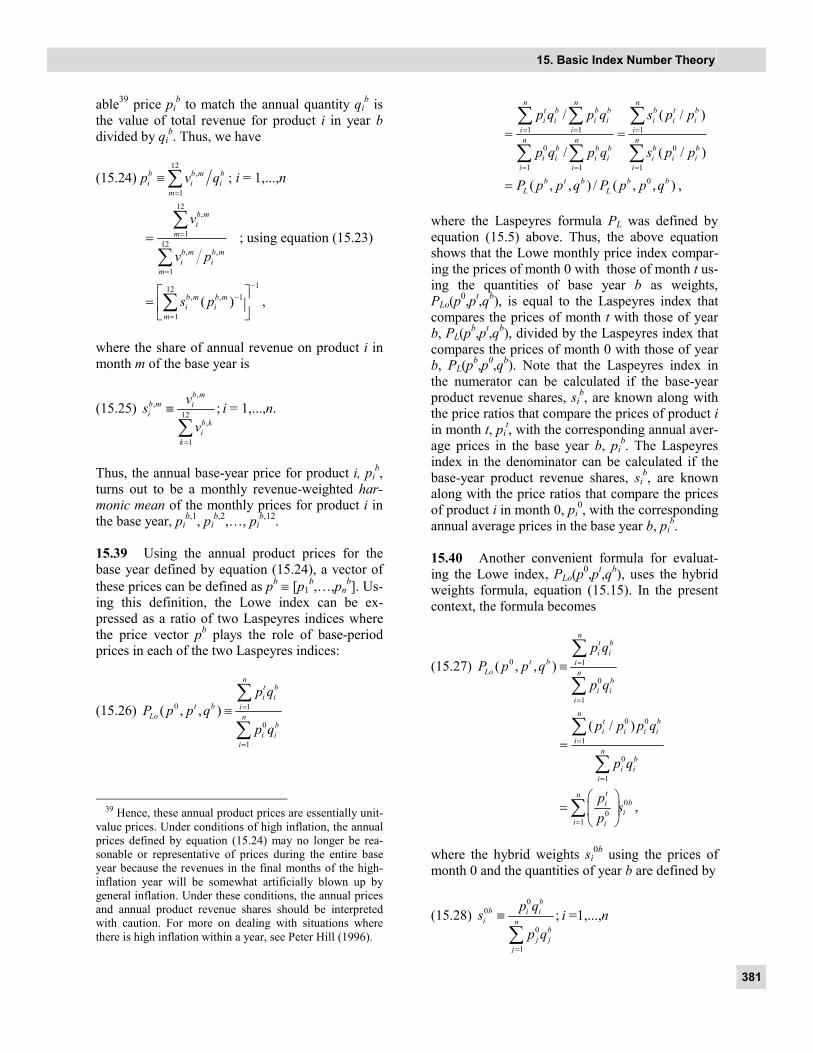
15. Basic Index Number Theory
381
able39 price pib to match the annual quantity qi
b is the value of total revenue for product i in year b divided by qi
b. Thus, we have
(15.24)12
,
1
b b m bi i i
mp v q
=
≡ ∑ ; i = 1,...,n
12,
112
, ,
1
b mi
m
b m b mi i
m
v
v p
=
=
=∑
∑; using equation (15.23)
112, , 1
1
( )b m b mi i
m
s p−
−
=
=
∑ ,
where the share of annual revenue on product i in month m of the base year is
(15.25) ,
,12
,
1
;b m
b m ii
b ki
k
vs
v=
≡
∑i = 1,...,n.
Thus, the annual base-year price for product i, pi
b, turns out to be a monthly revenue-weighted har-monic mean of the monthly prices for product i in the base year, pi
b,1, pib,2,…, pi
b,12. 15.39 Using the annual product prices for the base year defined by equation (15.24), a vector of these prices can be defined as pb ≡ [p1
b,…,pnb]. Us-
ing this definition, the Lowe index can be ex-pressed as a ratio of two Laspeyres indices where the price vector pb plays the role of base-period prices in each of the two Laspeyres indices:
(15.26) 0 1
0
1
( , , )
nt bi i
t b iLo n
bi i
i
p qP p p q
p q
=
=
≡∑
∑
39 Hence, these annual product prices are essentially unit-
value prices. Under conditions of high inflation, the annual prices defined by equation (15.24) may no longer be rea-sonable or representative of prices during the entire base year because the revenues in the final months of the high-inflation year will be somewhat artificially blown up by general inflation. Under these conditions, the annual prices and annual product revenue shares should be interpreted with caution. For more on dealing with situations where there is high inflation within a year, see Peter Hill (1996).
1 1 1
0 0
1 1 1
/ ( / )
/ ( / )
n n nt b b b b t bi i i i i i i
i i in n n
b b b b bi i i i i i i
i i i
p q p q s p p
p q p q s p p
= = =
= = =
= =∑ ∑ ∑
∑ ∑ ∑
0( , , ) / ( , , )b t b b bL LP p p q P p p q= ,
where the Laspeyres formula PL was defined by equation (15.5) above. Thus, the above equation shows that the Lowe monthly price index compar-ing the prices of month 0 with those of month t us-ing the quantities of base year b as weights, PLo(p0,pt,qb), is equal to the Laspeyres index that compares the prices of month t with those of year b, PL(pb,pt,qb), divided by the Laspeyres index that compares the prices of month 0 with those of year b, PL(pb,p0,qb). Note that the Laspeyres index in the numerator can be calculated if the base-year product revenue shares, si
b, are known along with the price ratios that compare the prices of product i in month t, pi
t, with the corresponding annual aver-age prices in the base year b, pi
b. The Laspeyres index in the denominator can be calculated if the base-year product revenue shares, si
b, are known along with the price ratios that compare the prices of product i in month 0, pi
0, with the corresponding annual average prices in the base year b, pi
b. 15.40 Another convenient formula for evaluat-ing the Lowe index, PLo(p0,pt,qb), uses the hybrid weights formula, equation (15.15). In the present context, the formula becomes
(15.27) 0 1
0
1
( , , )
nt bi i
t b iLo n
bi i
i
p qP p p q
p q
=
=
≡∑
∑
0 0
1
0
1
( / )n
t bi i i i
in
bi i
i
p p p q
p q
=
=
=∑
∑
00
1
tnbi
ii i
ps
p=
=
∑ ,
where the hybrid weights si
0b using the prices of month 0 and the quantities of year b are defined by
(15.28) 0
0
0
1
;b
b i ii n
bj j
j
p qsp q
=
≡
∑i =1,...,n

Producer Price Index Manual
382
0
0
1
( / ) .( / )
b b bi i i i
nb b bj j j j
j
p q p p
p q p p=
= ∑
Equation (15.28) shows how the base-year reve-nues, pi
bqib, can be multiplied by the product price
indices, pi0/pi
b, to calculate the hybrid shares. 15.41 One additional formula for the Lowe in-dex, PLo(p0,pt,qb), will be exhibited. Note that the Laspeyres decomposition of the Lowe index de-fined by the third line in equation (15.26) involves the very long-term price relatives, pi
t/pib, that com-
pare the prices in month t, pit, with the possibly
distant base-year prices, pib. Further, the hybrid
share decomposition of the Lowe index defined by the third line in equation (15.27) involves the long-term monthly price relatives, pi
t/pi0, which com-
pare the prices in month t, pit, with the base month
prices, pi0. Both these formulas are not satisfactory
in practice because of the problem of sample attri-tion: each month, a substantial fraction of products disappears from the marketplace, and thus it is use-ful to have a formula for updating the previous month’s price index using just month-over-month price relatives. In other words, long-term price relatives disappear at a rate that is too large in practice to base an index number formula on their use. The Lowe index for month t + 1, PLo(p0,pt+1,qb), can be written in terms of the Lowe index for month t, PLo(p0,pt,qb), and an updating factor as follows:
(15.29)
1
0 1 1
0
1
( , , )
nt bi i
t b iLo n
bi i
i
p qP p p q
p q
+
+ =
=
≡∑
∑
1
1 1
0
1 1
n nt b t bi i i i
i in n
b t bi i i i
i i
p q p q
p q p q
+
= =
= =
=
∑ ∑
∑ ∑
1
0 1
1
( , , )
nt bi i
t b iLo n
t bi i
i
p qP p p q
p q
+
=
=
=
∑
∑
1
10
1
( , , )
tnt bii it
i it bLo n
t bi i
i
p p qp
P p p qp q
+
=
=
=
∑
∑
10
1
( , , )tn
t b tbiLo it
i i
pP p p q s
p
+
=
=
∑ ,
where the hybrid weights si
tb are defined by
(15.30)
1
;t b
tb i ii n
t bj j
j
p qsp q
=
≡
∑i =1,...,n.
Thus, the required updating factor, going from month t to month t + 1, is the chain-linked index
( )1
1
ntb t ti i i
i
s p p+
=∑ , which uses the hybrid share
weights sitb corresponding to month t and base
year b. 15.42 The Lowe index PLo(p0,pt,qb) can be re-garded as an approximation to the ordinary Laspeyres index, PL(p0,pt,q0), that compares the prices of the base month 0, p0, with those of month t, pt, using the quantity vector of month 0, q0, as weights. There is a relatively simple formula that relates these two indices. To explain this for-mula, it is first necessary to make a few defini-tions. Define the ith price relative between month 0 and month t as
(15.31) 0/ ;ti i ir p p≡ i =1,...,n.
The ordinary Laspeyres price index, going from month 0 to t, can be defined in terms of these price relatives as follows:
(15.32)
0
0 0 1
0 0
1
( , , )
nti i
t iL n
i ii
p qP p p q
p q
=
=
≡∑
∑
0 00
1 00
0 0 1
1
tni
i i tni i i
ini i
i ii
p p qp p
spp q
=
=
=
= =
∑∑
∑
15. Basic Index Number Theory
383
0
1
n
i ii
s r r∗
=
= ≡∑ ,
where the month 0 revenue shares si
0 are defined as follows:
(15.33) 0 0
0
0 0
1
;i ii n
j jj
p qsp q
=
≡
∑i =1,...,n.
15.43 Define the ith quantity relative ti as the ra-tio of the quantity of product i used in the base year b, qi
b, to the quantity used in month 0, qi0, as
follows:
(15.34) 0/ ;bi i it q q≡ i =1,...,n.
The Laspeyres quantity index, QL(q0,qb,p0), that compares quantities in year b, qb, with the corre-sponding quantities in month 0, q0, using the prices of month 0, p0, as weights can be defined as a weighted average of the quantity ratios ti as follows:
(15.35)
0
0 0 1
0 0
1
( , , )
nb
i ib i
L n
i ii
p qQ q q p
p q
=
=
≡∑
∑
0 00
1
0 0
1
bni
i ii i
n
i ii
q p qq
p q
=
=
=
∑
∑
00
1
bni
ii i
qs
q=
=
∑ ; using equation (15.34)
01
*ni ii
s t t=
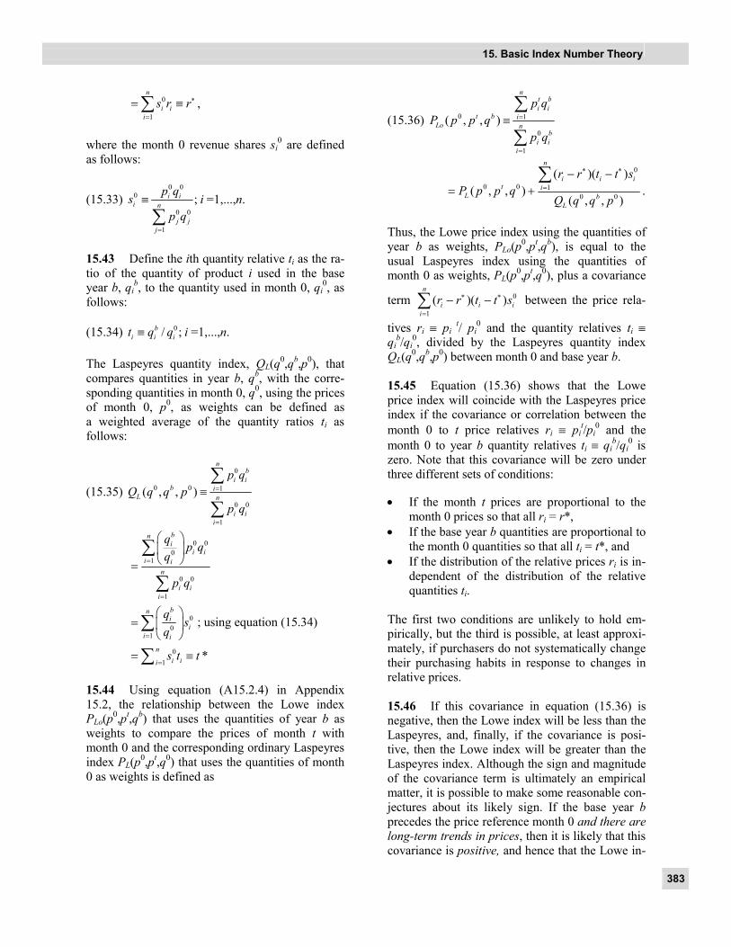
= ≡∑ 15.44 Using equation (A15.2.4) in Appendix 15.2, the relationship between the Lowe index PLo(p0,pt,qb) that uses the quantities of year b as weights to compare the prices of month t with month 0 and the corresponding ordinary Laspeyres index PL(p0,pt,q0) that uses the quantities of month 0 as weights is defined as
(15.36) 0 1
0
1
( , , )
nt bi i
t b iLo n
bi i
i
p qP p p q
p q
=
=
≡∑
∑
0
0 0 10 0
( )( )( , , )
( , , )
n
i i it i
L bL
r r t t sP p p q
Q q q p
∗ ∗
=
− −= +
∑.
Thus, the Lowe price index using the quantities of year b as weights, PLo(p0,pt,qb), is equal to the usual Laspeyres index using the quantities of month 0 as weights, PL(p0,pt,q0), plus a covariance
term 0
1
( )( )n
i i ii
r r t t s∗ ∗
=
− −∑ between the price rela-
tives ri ≡ pi t/ pi
0 and the quantity relatives ti ≡ qi
b/qi0, divided by the Laspeyres quantity index
QL(q0,qb,p0) between month 0 and base year b. 15.45 Equation (15.36) shows that the Lowe price index will coincide with the Laspeyres price index if the covariance or correlation between the month 0 to t price relatives ri ≡ pi
t/pi0 and the
month 0 to year b quantity relatives ti ≡ qib/qi
0 is zero. Note that this covariance will be zero under three different sets of conditions:
• If the month t prices are proportional to the month 0 prices so that all ri = r*,
• If the base year b quantities are proportional to the month 0 quantities so that all ti = t*, and
• If the distribution of the relative prices ri is in-dependent of the distribution of the relative quantities ti.
The first two conditions are unlikely to hold em-pirically, but the third is possible, at least approxi-mately, if purchasers do not systematically change their purchasing habits in response to changes in relative prices. 15.46 If this covariance in equation (15.36) is negative, then the Lowe index will be less than the Laspeyres, and, finally, if the covariance is posi-tive, then the Lowe index will be greater than the Laspeyres index. Although the sign and magnitude of the covariance term is ultimately an empirical matter, it is possible to make some reasonable con-jectures about its likely sign. If the base year b precedes the price reference month 0 and there are long-term trends in prices, then it is likely that this covariance is positive, and hence that the Lowe in-

Producer Price Index Manual
384
dex will exceed the corresponding Laspeyres price index;40 that is,
(15.37) 0 0 0( , , ) ( , , ).t b tLo LP p p q P p p q>
To see why this covariance is likely to be positive, suppose that there is a long-term upward trend in the price of product i so that ri − r* ≡ (pi
t / pi0) − r*
is positive. With normal substitution responses,41 qi
t / qi0 less an average quantity change of this type
(t*) is likely to be negative, or, upon taking recip-rocals, qi
0 / qit less an average quantity change of
this (reciprocal) type is likely to be positive. But if the long-term upward trend in prices has persisted back to the base year b, then ti − t* ≡ (qi
b / qi0) − t*
is also likely to be positive. Hence, the covariance will be positive under these circumstances. More-over, the more distant is the weight reference year b from the price reference month 0, the bigger the residuals ti − t* will likely be and the bigger will be the positive covariance. Similarly, the more dis-tant is the current-period month t from the base-period month 0, the bigger the residuals ri − r* will likely be and the bigger will be the positive covari-ance. Thus, under the assumptions that there are long-term trends in prices and normal substitution responses, the Lowe index will normally be greater than the corresponding Laspeyres index. 15.47 Define the Paasche index between months 0 and t as follows:
40It is also necessary to assume that purchasers have nor-
mal substitution effects in response to these long-term trends in prices; that is, if a product increases (relatively) in price, its quantity purchased will decline (relatively), and if a product decreases relatively in price, its quantity pur-chased will increase relatively. This reflects the normal “market equilibrium” response to changes in supply.
41Walsh (1901, pp. 281–82) was well aware of substitu-tion effects, as can be seen in the following comment that noted the basic problem with a fixed-basket index that uses the quantity weights of a single period: “The argument made by the arithmetic averagist supposes that we buy the same quantities of every class at both periods in spite of the variation in their prices, which we rarely, if ever, do. As a rough proposition, we—a community—generally spend more on articles that have risen in price and get less of them, and spend less on articles that have fallen in price and get more of them.”
(15.38) 0 1
0
1
( , , ) .
nt ti i
t t iP n
ti i
i
p qP p p q
p q
=
=
≡∑
∑
As was discussed in Section C.1, a reasonable tar-get index to measure the price change going from month 0 to t is some sort of symmetric average of the Paasche index PP(p0,pt,qt) defined by equation (15.38) and the corresponding Laspeyres index PL(p0,pt,q0) defined by equation (15.32). Adapting equation (A15.1.5) in Appendix 15.1, the relation-ship between the Paasche and Laspeyres indices can be written as follows: (15.39) 0 0 0( , , ) ( , , )t t t
P LP p p q P p p q=
0
10 0
( )( )
( , , )
n
i i ii
tL
r r u u s
Q q q p
∗ ∗
=
− −+
∑,
where the price relatives ri ≡ pi
t / pi0 are defined by
equation (15.31) and their share-weighted average r* by equation (15.32), and the ui, u* and QL are defined as follows: (15.40) 0/ ;t
i i iu q q≡ i = 1,...,n,
(15.41) 0 0 0
1
( , , )n
ti i L
i
u s u Q q q p∗
=
≡ =∑ ,
and the month 0 revenue shares si
0 are defined by equation (15.33). Thus, u* is equal to the Laspeyres quantity index between months 0 and t. This means that the Paasche price index that uses the quantities of month t as weights, PP(p0,pt,qt), is equal to the usual Laspeyres index using the quan-tities of month 0 as weights, PL(p0,pt,q0), plus a
covariance term 0
1
( )( )n
i i ii
r r u u s∗ ∗
=
− −∑ between the
price relatives ri ≡ pit / pi
0 and the quantity relatives ui ≡ qi
t / qi0, divided by the Laspeyres quantity in-
dex QL(q0,qt,p0) between month 0 and month t. 15.48 Although the sign and magnitude of the covariance term is again an empirical matter, it is possible to make a reasonable conjecture about its likely sign. If there are long-term trends in prices, and purchasers respond normally to price changes in their purchases, then it is likely that this covari-

15. Basic Index Number Theory
385
ance is negative, and hence the Paasche index will be less than the corresponding Laspeyres price in-dex; that is,
(15.42) 0 0 0( , , ) ( , , )t t tP LP p p q P p p q< .
To see why this covariance is likely to be negative, suppose that there is a long-term upward trend in the price of product i 42 so that ri − r* ≡ (pi
t / pi0) −
r* is positive. With normal substitution responses, qi
t / qi0 less an average quantity change of this type
(u*) is likely to be negative. Hence, ui − u* ≡ (qit /
qi0) − u* is likely to be negative. Thus, the covari-
ance will be negative under these circumstances. Moreover, the more distant is the base month 0 from the current-month t, the bigger in magnitude the residuals ui − u* will likely be and the bigger in magnitude will be the negative covariance.43 Simi-larly, the more distant is the current-period month t from the base-period month 0, the bigger the re-siduals ri − r* will likely be and the bigger in mag-nitude will be the covariance. Thus, under the as-sumptions that there are long-term trends in prices and normal substitution responses, the Laspeyres index will be greater than the corresponding Paasche index, with the divergence likely growing as month t becomes more distant from month 0. 15.49 Putting the arguments in the three previ-ous paragraphs together, it can be seen that under the assumptions that there are long-term trends in prices and normal substitution responses, the Lowe price index between months 0 and t will exceed the corresponding Laspeyres price index, which in turn will exceed the corresponding Paasche price index; that is, under these hypotheses,
(15.43) 0 0 0 0( , , ) ( , , ) ( , , ).t b t t t
Lo L PP p p q P p p q P p p q> > Thus, if the long-run target price index is an aver-age of the Laspeyres and Paasche indices, it can be
42The reader can carry through the argument if there is a long-term relative decline in the price of the ith product. The argument required to obtain a negative covariance re-quires that there be some differences in the long-term trends in prices; that is, if all prices grow (or fall) at the same rate, we have price proportionality, and the covari-ance will be zero.
43However, QL = u* may also be growing in magnitude, so the net effect on the divergence between PL and PP is ambiguous.
seen that the Laspeyres index will have an upward bias relative to this target index, and the Paasche index will have a downward bias. In addition, if the base year b is prior to the price reference month, month 0, then the Lowe index will also have an upward bias relative to the Laspeyres in-dex and hence also to the target index. D.2 Lowe index and midyear indices
15.50 The discussion in the previous paragraph assumed that the base year b for quantities pre-ceded the base month for prices, month 0. How-ever, if the current-period month t is quite distant from the base month 0, then it is possible to think of the base year b as referring to a year that lies be-tween months 0 and t. If the year b does fall be-tween months 0 and t, then the Lowe index be-comes a midyear index.44 The Lowe midyear index no longer has the upward biases indicated by the inequalities in equation (15.43) under the assump-tion of long-term trends in prices and normal sub-stitution responses by quantities.
15.51 It is now assumed that the base-year quan-tity vector qb corresponds to a year that lies be-tween months 0 and t. Under the assumption of long-term trends in prices and normal substitution effects so that there are also long-term trends in quantities (in the opposite direction to the trends in prices so that if the ith product price is trending up, then the corresponding ith quantity is trending down), it is likely that the intermediate-year quan-
44This concept can be traced to Peter Hill (1998, p. 46):
“When inflation has to be measured over a specified se-quence of years, such as a decade, a pragmatic solution to the problems raised above would be to take the middle year as the base year. This can be justified on the grounds that the basket of goods and services purchased in the middle year is likely to be much more representative of the pattern of consumption over the decade as a whole than baskets purchased in either the first or the last years. Moreover, choosing a more representative basket will also tend to re-duce, or even eliminate, any bias in the rate of inflation over the decade as a whole as compared with the increase in the CoL index.” Thus, in addition to introducing the con-cept of a midyear index, Hill also introduced the idea of representativity bias. For additional material on midyear indices, see Schultz (1999) and Okamoto (2001). Note that the midyear index concept could be viewed as a close com-petitor to Walsh’s (1901, p. 431) multiyear fixed-basket in-dex, where the quantity vector was chosen to be an arith-metic or geometric average of the quantity vectors in the period.

Producer Price Index Manual
386
tity vector will lie between the monthly quantity vectors q0 and qt. The midyear Lowe index, PLo(p0,pt,qb), and the Laspeyres index going from month 0 to t, PL(p0,pt,q0), will still satisfy the exact relationship given by equation (15.36). Thus, PLo(p0,pt,qb) will equal PL(p0,pt,q0) plus the co-
variance term 0 0 0
1
( )( ) ( , , )n
bi i i L
i
r r t t s Q q q p∗ ∗
=
− −∑ ,
where QL(q0,qb,p0) is the Laspeyres quantity index going from month 0 to t. This covariance term is likely to be negative, so that
(15.44) 0 0 0( , , ) ( , , ).t t bL LoP p p q P p p q>
To see why this covariance is likely to be negative, suppose that there is a long-term upward trend in the price of product i so that ri − r* ≡ (pi
t / pi0) − r*
is positive. With normal substitution responses, qi will tend to decrease relatively over time, and since qi
b is assumed to be between qi0 and qi
t, qi
b/qi0 less an average quantity change of this type,
r* is likely to be negative. Hence ui − u* ≡ (qi
b / qi0) − t* is likely to be negative. Thus, the co-
variance is likely to be negative under these cir-cumstances. Under the assumptions that the quan-tity base year falls between months 0 and t and that there are long-term trends in prices and nor-mal substitution responses, the Laspeyres index will normally be larger than the corresponding Lowe midyear index, with the divergence likely growing as month t becomes more distant from month 0. 15.52 It can also be seen that under the above assumptions, the midyear Lowe index is likely to be greater than the Paasche index between months 0 and t; that is,
(15.45) 0 0( , , ) ( , , ).t b t tLo PP p p q P p p q>
To see why the above inequality is likely to hold, think of qb starting at the month 0 quantity vector q0 and then trending smoothly to the month t quan-tity vector qt. When qb = q0, the Lowe index be-comes the Laspeyres index PL(p0,pt,q0). When qb = qt, the Lowe index becomes the Paasche index PP(p0,pt,qt). Under the assumption of trending prices and normal substitution responses to these trending prices, it was shown earlier that the Paasche index will be less than the corresponding Laspeyres price index; that is, that PP(p0,pt,qt) was less than PL(p0,pt,q0); recall equation (15.42).
Thus, under the assumption of smoothly trending prices and quantities between months 0 and t, and assuming that qb is between q0 and qt, we will have (15.46) 0 0( , , ) ( , , )t t t b
P LoP p p q P p p q< 0 0( , , )t
LP p p q< . Thus, if the base year for the Lowe index is chosen to be between the base month for the prices, month 0, and the current month for prices, month t, and there are trends in prices with corresponding trends in quantities that correspond to normal substitution effects, then the resulting Lowe index is likely to lie between the Paasche and Laspeyres indices go-ing from months 0 to t. If the trends in prices and quantities are smooth, then choosing the base year halfway between periods 0 and t should give a Lowe index that is approximately halfway between the Paasche and Laspeyres indices and hence will be very close to an ideal target index between months 0 and t. This basic idea has been imple-mented by Okamoto (2001) using Japanese con-sumer data, and he found that the resulting mid-year indices approximated the corresponding Fisher ideal indices very closely. 15.53 It should be noted that these midyear indi-ces can be computed only on a retrospective basis; that is, they cannot be calculated in a timely fash-ion as can Lowe indices that use a base year before month 0. Thus, midyear indices cannot be used to replace the more timely Lowe indices. However, these timely Lowe indices are likely to have an upward bias even bigger than the usual Laspeyres upward bias compared with an ideal target index, which was taken to be an average of the Paasche and Laspeyres indices.
15.54 All of the inequalities derived in this sec-tion rest on the assumption of long-term trends in prices (and corresponding economic responses in quantities). If there are no systematic long-run trends in prices and only random fluctuations around a common trend in all prices, then the above inequalities are not valid, and the Lowe in-dex using a prior base year will probably provide a perfectly adequate approximation to both the Paasche and Laspeyres indices. However, there are some reasons for believing that some long-run trends in prices exist:
15. Basic Index Number Theory
387
(i) The computer chip revolution of the past 40 years has led to strong downward trends in the prices of products that use these chips in-tensively. As new uses for chips are devel-oped, the share of products that are chip-intensive has grown, which implies that what used to be a relatively minor problem has be-come a major problem.
(ii) Other major scientific advances have had similar effects. For example, the invention of fiber-optic cable (and lasers) has led to a downward trend in telecommunications prices as obsolete technologies based on copper wire are gradually replaced.
(iii) Since the end of World War II, a series of in-ternational trade agreements have dramati-cally reduced tariffs around the world. These reductions, combined with improvements in transportation technologies, have led to a rapid growth of international trade and re-markable improvements in international spe-cialization. Manufacturing activities in the more developed economies have gradually been outsourced to lower-wage countries, leading to deflation in goods prices in most countries. However, many services cannot be readily outsourced,45 and so on average the price of services trends upward while the price of goods trends downward.
(iv) At the microeconomic level, there are tre-mendous differences in growth rates of firms. Successful firms expand their scale, lower their costs, and cause less successful competi-tors to wither away with their higher prices and lower volumes. This leads to a systematic negative correlation between changes in item prices and the corresponding changes in item volumes that can be very large.
Thus, there is some a priori basis for assuming long-run divergent trends in prices and hence some basis for concern that a Lowe index that uses a base year for quantity weights that is prior to the base month for prices may be upward biased, compared with a more ideal target index.
45However some services can be internationally out-
sourced; for example, call centers, computer programming, and airline maintenance.
D.3 Young index
15.55 Recall the definitions for the base-year quantities, qi
b, and the base-year prices, pib, given
by equation (15.23) and equation (15.24). The base-year revenue shares can be defined in the usual way as follows:
(15.47)
1
;b b
b i ii n
b bk k
k
p qs
p q=
≡
∑i =1,...,n.
Define the vector of base-year revenue shares in the usual way as sb ≡ [s1
b,…,snb]. These base-year
revenue shares were used to provide an alternative formula for the base year b Lowe price index go-ing from month 0 to t defined in equation (15.26)
as PLo(p0,pt,qb) = 0
1 1
( / ) ( / )n n
b t b b bi i i i i i
i i
s p p s p p= =∑ ∑ .
Rather than using this index as their short-run tar-get index, many statistical agencies use the follow-ing closely related index:
(15.48) ( )0 0
1
( , , ) .n
t b b tY i i i
i
P p p s s p p=
≡ ∑
This type of index was first defined by the English economist Arthur Young (1812).46 Note that there is a change in focus when the Young index is used compared with the indices proposed earlier in this chapter. Up to this point, the indices proposed have been of the fixed-basket type (or averages of such indices), where a product basket that is somehow representative for the two periods being compared is chosen and then “purchased” at the prices of the two periods, and the index is taken to be the ratio of these two costs. On the other hand, for the Young index, one instead chooses representative revenue shares that pertain to the two periods un-der consideration and then uses these shares to cal-culate the overall index as a share-weighted aver-age of the individual price ratios, pi
t / pi0. Note that
this share-weighted average of price ratios view of index number theory is a bit different from the view taken at the beginning of this chapter, which viewed the index number problem as the problem of decomposing a value ratio into the product of two terms, one of which expresses the amount of
46Walsh (1901, p. 536; 1932, p. 657) attributes this for-mula to Young.

Producer Price Index Manual
388
price change between the two periods and the other that expresses the amount of quantity change.47 15.56 Statistical agencies sometimes regard the Young index defined above as an approximation to the Laspeyres price index PL(p0,pt,q0). Hence, it is of interest to see how the two indices compare. De-fining the long-term monthly price relatives going from month 0 to t as ri ≡ pi
t/pi0 and using equations
(15.32) and (15.48),
(15.49) 0 0 0( , , ) ( , , )t b tY LP p p s P p p q−
00 0
1 1
t tn nb i ii i
i ii i
p ps s
p p= =
≡ −
∑ ∑
0 00
1 1
0 0
1 1
0
1,
tn nb bii i i i i
i ii
n nb bi i i i i
i i
nbi i i
i
ps s s s r
p
s s r r r s s
s s r r
= =
∗ ∗
= =
∗
=
= − = −
= − − + −
= − −
∑ ∑
∑ ∑
∑
since 0
1 1
1n n
bi i
i i
s s= =
= =∑ ∑ and defining
47Irving Fisher’s 1922 book is famous for developing the
value ratio decomposition approach to index number the-ory, but his introductory chapters took the share-weighted average point of view: “An index number of prices, then, shows the average percentage change of prices from one point of time to another” (1922, p. 3). Fisher went on to note the importance of economic weighting: “The preced-ing calculation treats all the commodities as equally impor-tant; consequently, the average was called ‘simple’. If one commodity is more important than another, we may treat the more important as though it were two or three com-modities, thus giving it two or three times as much ‘weight’ as the other commodity” (1922, p. 6). Walsh (1901, pp. 430–31) considered both approaches: “We can either (1) draw some average of the total money values of the classes during an epoch of years, and with weighting so determined employ the geometric average of the price variations [ra-tios]; or (2) draw some average of the mass quantities of the classes during the epoch, and apply to them Scrope’s method.” Scrope’s method is the same as using the Lowe index. Walsh (1901, pp. 88–90) consistently stressed the importance of weighting price ratios by their economic im-portance (rather than using equally weighted averages of price relatives). Both the value ratio decomposition ap-proach and the share-weighted average approach to index number theory will be studied from the axiomatic perspec-tive in the following chapter; see also Sections C and E in Chapter 16.
( )0 0 0
1
* , ,n
ti i L
i
r s r P p p q=
≡ =∑ .
Thus, the Young index PY(p0,pt,sb) is equal to the Laspeyres index PL(p0,pt,q0) plus the covariance between the difference in the annual shares per-taining to year b and the month 0 shares, si
b − si0,
and the deviations of the relative prices from their mean, ri − r*. 15.57 It is no longer possible to guess the likely sign of the covariance term. The question is no longer whether the quantity demanded goes down as the price of product i goes up (the answer to this question is usually yes) but does the share of reve-nue go down as the price of product i goes up? The answer depends on the elasticity of demand for the product. However, let us provisionally assume that there are long-run trends in product prices, and if the trend in prices for product i is above the mean, then the revenue share for the product trends down (and vice versa). Thus, we are assuming high elas-ticities or very strong substitution effects. Assum-ing also that the base year b is before month 0, then under these conditions, suppose that there is a long-term upward trend in the price of product i so that ri − r* ≡ (pi
t / pi0) − r* is positive. With the as-
sumed very elastic purchaser substitution re-sponses, si will tend to decrease relatively over time. Since si
b is assumed to be before si0, si
0 is ex-pected to be less than si
b , or sib − si
0 will likely be positive. Thus, the covariance is likely to be posi-tive under these circumstances. Hence with long-run trends in prices and very elastic responses of purchasers to price changes, the Young index is likely to be greater than the corresponding Laspeyres index.
15.58 Assume that there are long-run trends in product prices. If the trend in prices for product i is above the mean, then suppose that the revenue share for the product trends up (and vice versa). Thus, we are assuming low elasticities or very weak substitution effects. Assume also that the base year b is before month 0, and suppose that there is a long-term upward trend in the price of product i so that ri − r* ≡ (pi
t / pi0) − r* is positive.
With the assumed very inelastic substitution re-sponses, si will tend to increase relatively over time, and, since si
b is assumed to be before si0, we
will have si0 greater than si
b , or sib − si
0 is negative. Thus, the covariance is likely to be negative under
15. Basic Index Number Theory
389
these circumstances. Hence with long-run trends in prices and very inelastic responses of purchasers to price changes, the Young index is likely to be less than the corresponding Laspeyres index.
15.59 The previous two paragraphs indicate that, a priori, it is not known what the likely difference between the Young index and the corresponding Laspeyres index will be. If elasticities of substitu-tion are close to 1, then the two sets of revenue shares, si
b and si0, will be close to each other and
the difference between the two indices will be close to zero. However, if monthly revenue shares have strong seasonal components, then the annual shares si
b could differ substantially from the monthly shares si
0.
15.60 It is useful to have a formula for updating the previous month’s Young price index using only month-over-month price relatives. The Young index for month t + 1, PY(p0,pt+1,sb), can be pre-sented in terms of the Lowe index for month t, PY(p0,pt,sb), and an updating factor as follows:
(15.50) 1
0 10
1( , , )
tnt b b i
Y ii i
pP p p s s
p
++
=
≡
∑
1 0
0 1
0
1
( / )( , , )
( / )
nb ti i i
t b iY n
b ti i i
i
s p pP p p s
s p p
+
=
=
=∑
∑
1 0
0 1
0
1
( / )( , , )
( / )
nb b ti i i i
t b iY n
b b ti i i i
i
p q p pP p p s
p q p p
+
=
=
=∑
∑;
using equation (15.47) 1
010
0
1
0 0 1
1
( , , )( / )
( , , ) ( / ) ,
t tnb b i ii i t
i i it bY n
b b ti i i i
i
nt b b t t t
Y i i ii
p pp qp p
P p p sp q p p
P p p s s p p
+
=
=
+
=
=
=
∑
∑
∑
where the hybrid weights si
b0t are defined by
(15.51) 0
0
0
1
( / )
( / )
b b tb t i i i ii n
b b tk k k k
k
p q p ps
p q p p=
≡
∑
0
0
1
( / );
( / )
b ti i i
nb tk k k
k
s p p
s p p=
=
∑i = 1,...,n.
Thus, the hybrid weights si
b0t can be obtained from the base-year weights si
b by updating them; that is, by multiplying them by the price relatives (or indi-ces at higher levels of aggregation), pi
t / pi0. Thus,
the required updating factor, going from month t to month t + 1, is the chain-linked index,
0 1
1
( / )n
b t t ti i i
i
s p p+
=∑ , which uses the hybrid revenue-
share weights sib0t defined by equation (15.51).
15.61 Even if the Young index provides a close approximation to the corresponding Laspeyres in-dex, it is difficult to recommend the use of the Young index as a final estimate of the change in prices going from period 0 to t, just as it was diffi-cult to recommend the use of the Laspeyres index as the final estimate of inflation going from period 0 to t. Recall that the problem with the Laspeyres index was its lack of symmetry in the treatment of the two periods under consideration. That is, using the justification for the Laspeyres index as a good fixed-basket index, there was an identical justifica-tion for the use of the Paasche index as an equally good fixed-basket index to compare periods 0 and t. The Young index suffers from a similar lack of symmetry with respect to the treatment of the base period. The problem can be explained as follows. The Young index, PY(p0,pt,sb), defined by equation (15.48), calculates the price change between months 0 and t, treating month 0 as the base. But there is no particular reason to treat month 0 as the base month other than convention. Hence, if we treat month t as the base and use the same formula to measure the price change from month t back to
month 0, the index PY(p0,pt,sb) = 0
1
( / )n
b ti i i
i
s p p=∑
would be appropriate. This estimate of price change can then be made comparable to the origi-nal Young index by taking its reciprocal, leading to the following rebased Young index,48 PY*(p0,pt,sb), defined as
48Using Irving Fisher’s (1922, p. 118) terminology,
PY*(p0,pt,sb) ≡ 1/[PY(pt,p0,sb)] is the time antithesis of the original Young index, PY(p0,pt,sb).
Producer Price Index Manual
390
(15.52) 0 0
1
( , , ) 1 ( / )n
t b b tY i i i
i
P p p s s p p∗
=
≡ ∑
1
0 1
1
( / ) .n
b ti i i
i
s p p−
−
=
=
∑
Thus, the rebased Young index, PY*(p0,pt,sb), that uses the current month as the initial base period is a share-weighted harmonic mean of the price rela-tives going from month 0 to month t, whereas the original Young index, PY(p0,pt,sb), is a share-weighted arithmetic mean of the same price rela-tives. 15.62 Fisher argued that an index number for-mula should give the same answer no matter which period was chosen as the base:
Either one of the two times may be taken as the “base”. Will it make a difference which is cho-sen? Certainly, it ought not and our Test 1 de-mands that it shall not. More fully expressed, the test is that the formula for calculating an index number should be such that it will give the same ratio between one point of comparison and the other point, no matter which of the two is taken as the base. (Irving Fisher, 1922, p. 64)
15.63 The problem with the Young index is that not only does it not coincide with its rebased coun-terpart, but there is a definite inequality between the two indices, namely
(15.53) 0 0( , , ) ( , , ),t b t bY YP p p s P p p s∗ ≤
with a strict inequality provided that the period t price vector pt is not proportional to the period 0 price vector p0.49 Thus, a statistical agency that
49These inequalities follow from the fact that a harmonic
mean of M positive numbers is always equal to or less than the corresponding arithmetic mean; see Walsh (1901, p. 517) or Irving Fisher (1922, pp. 383–84). This inequality is a special case of Schlömilch’s (1858) Inequality; see Hardy, Littlewood and Polyá (1934, p. 26). Walsh (1901, pp. 330–32) explicitly noted the inequality in equation (15.53) and also noted that the corresponding geometric average would fall between the harmonic and arithmetic averages. Walsh (1901, p. 432) computed some numerical examples of the Young index and found big differences be-tween it and his best indices, even using weights that were representative for the periods being compared. Recall that the Lowe index becomes the Walsh index when geometric
(continued)
uses the direct Young index PY(p0,pt,sb) will gener-ally show a higher inflation rate than a statistical agency that uses the same raw data but uses the re-based Young index, PY*(p0,pt,sb). 15.64 The inequality in equation (15.53) does not tell us by how much the Young index will ex-ceed its rebased time antithesis. However, in Ap-pendix 15.3, it is shown that to the accuracy of a certain second-order Taylor series approximation, the following relationship holds between the direct Young index and its time antithesis:
(15.54) 0 0( , , ) ( , , )t b t bY YP p p s P p p s∗≈
0( , , ) Var ,t bYP p p s e+
where Var e is defined as
(15.55) 2
1
Var .n
bi i
i
e s e e∗
=
≡ − ∑
The deviations ei are defined by 1 + ei = ri / r* for i = 1,…,n where the ri and their weighted mean r* are defined by (15.56) 0/ ;t
i i ir p p≡ i = 1,…,n ,
(15.57) 1
nbi i
i
r s r∗
=
≡ ∑ ,
which turns out to equal the direct Young index, PY(p0,pt,sb). The weighted mean of the ei is defined as
(15.58) 1
nbi i
i
e s e∗
=
≡ ∑ ,
which turns out to equal 0. Hence, the more dis-persion there is in the price relatives pi
t / pi0, to the
accuracy of a second-order approximation, the more the direct Young index will exceed its coun-terpart that uses month t as the initial base period rather than month 0.
mean quantity weights are chosen, and so the Lowe index can perform well when representative weights are used. This is not necessarily the case for the Young index, even using representative weights. Walsh (1901, p. 433) summed up his numerical experiments with the Young in-dex as follows: “In fact, Young’s method, in every form, has been found to be bad.”
15. Basic Index Number Theory
391
15.65 Given two a priori equally plausible index number formulas that give different answers, such as the Young index and its time antithesis, Irving Fisher (1922, p. 136) generally suggested taking the geometric average of the two indices.50 A benefit of this averaging is that the resulting for-mula will satisfy the time reversal test. Thus, rather than using either the base period 0 Young index, PY(p0,pt,sb), or the current period t Young index, PY*(p0,pt,sb), which is always below the base pe-riod 0 Young index if there is any dispersion in relative prices, it seems preferable to use the fol-lowing index, which is the geometric average of the two alternatively based Young indices:51
(15.59) 0( , , )t bYP p p s∗ ∗
1/20 0( , , ) ( , , ) .t b t b
Y YP p p s P p p s∗ ≡ If the base-year shares si
b happen to coincide with both the month 0 and month t shares, si
0 and sit, re-
spectively, the time-rectified Young index PY**(p0,pt,sb) defined by equation (15.59) will co-incide with the Fisher ideal price index between months 0 and t, PF(p0,pt,q0,qt) (which will also equal the Laspeyres and Paasche indices under these conditions). Note also that the index PY** de-fined by equation (15.59) can be produced on a timely basis by a statistical agency.
50“We now come to a third use of these tests, namely, to
‘rectify’ formulae, i.e., to derive from any given formula which does not satisfy a test another formula which does satisfy it; …. This is easily done by ‘crossing’, that is, by averaging antitheses. If a given formula fails to satisfy Test 1 [the time reversal test], its time antithesis will also fail to satisfy it; but the two will fail, as it were, in opposite ways, so that a cross between them (obtained by geometrical av-eraging) will give the golden mean which does satisfy” (Ir-ving Fisher, 1922, p. 136). Actually, the basic idea behind Fisher’s rectification procedure was suggested by Walsh, who was a discussant for Fisher (1921), where Fisher gave a preview of his 1922 book: “We merely have to take any index number, find its antithesis in the way prescribed by Professor Fisher, and then draw the geometric mean be-tween the two” (Correa Moylan Walsh, 1921b, p. 542).
51This index is a base-year weighted counterpart to an equally weighted index proposed by Carruthers, Sellwood, and Ward (1980, p. 25) and Dalén (1992a, p. 140) in the context of elementary index number formulas. See Chapter 20 for further discussion of this unweighted index.
E. Divisia Index and Discrete Approximations
E.1 Divisia price and quantity indices
15.66 The second broad approach to index num-ber theory relies on the assumption that price and quantity data change in a more or less continuous way.
15.67 Suppose that the price and quantity data on the n products in the chosen domain of defini-tion can be regarded as continuous functions of (continuous) time, say, pi(t) and qi(t) for i = 1,…,n. The value of producer revenue at time t is V(t) de-fined in the obvious way as
(15.60) 1
( ) ( ) ( ).n
i ii
V t p t q t=
≡ ∑
15.68 Now suppose that the functions pi(t) and qi(t) are differentiable. Then both sides of equation (15.60) can be differentiated with respect to time to obtain
(15.61) 1 1
( ) ( ) ( ) ( ) ( ).n n
i i i ii i
V t p t q t p t q t= =
′ ′′ = +∑ ∑
Divide both sides of equation (15.61) through by V(t) and, using equation (15.60), the following equation is obtained:
(15.62) 1 1
1
( ) ( ) ( ) ( )( ) / ( )
( ) ( )
n n
i i i ii i
n
j jj
p t q t p t q tV t V t
p t q t
= =
=
′ ′+′ =
∑ ∑
∑
1 1
( ) ( )( ) ( )
( ) ( )
n ni i
i ii ii i
p t q ts t s t
p t q t= =
′ ′= +∑ ∑ ,
where the time t revenue share on product i, si(t), is defined as
(15.63)
1
( ) ( )( )
( ) ( )
i ii n
m mm
p t q ts t
p t q t=
≡
∑for i = 1,…,n.
15.69 François Divisia (1926, p. 39) argued as follows: suppose the aggregate value at time t,
Producer Price Index Manual
392
V(t), can be written as the product of a time t price-level function, P(t), say, multiplied by a time t quantity-level function, Q(t), say; that is, we have
(15.64) ( ) ( ) ( ).V t P t Q t= Suppose, further, that the functions P(t) and Q(t) are differentiable. Then, differentiating equation (15.64) yields (15.65) ( ) ( ) ( ) ( ) ( ).V t P t Q t P t Q t′ ′ ′= + Dividing both sides of equation (15.65) by V(t) and using equation (15.64) leads to the following equation:
(15.66) ( ) ( ) ( ) .( ) ( ) ( )
V t P t Q tV t P t Q t
′ ′ ′ = +
15.70 Divisia compared the two expressions for the logarithmic value derivative, V′(t)/V(t), given by equation (15.62) and equation (15.66). He sim-ply defined the logarithmic rate of change of the aggregate price level, P′(t)/P(t), as the first set of terms on the right-hand side of equation (15.62), and he simply defined the logarithmic rate of change of the aggregate quantity level, Q′(t)/Q(t), as the second set of terms on the right-hand side of equation (15.62). That is, he made the following definitions:
(15.67) 1
( )( ) ( ) ;( ) ( )
ni
ii i
p tP t s tP t p t=
′′≡ ∑
(15.68) 1
( )( ) ( ) .( ) ( )
ni
ii i
q tQ t s tQ t q t=
′′≡ ∑
15.71 Equations (15.67) and (15.68) are reason-able definitions for the proportional changes in the aggregate price and quantity (or quantity) levels, P(t) and Q(t).52 The problem with these definitions is that economic data are not collected in continu-ous time; they are collected in discrete time. In other words, even though transactions can be
52If these definitions are applied (approximately) to the
Young index studied in the previous section, then it can be seen that for the Young price index to be consistent with the Divisia price index, the base-year shares should be cho-sen to be average shares that apply to the entire time period between months 0 and t.
thought of as occurring in continuous time, no producer records his or her purchases as they occur in continuous time; rather, purchases over a finite time period are cumulated and then recorded. A similar situation occurs for producers or sellers of products; firms cumulate their sales over discrete periods of time for accounting or analytical pur-poses. If it is attempted to approximate continuous time by shorter and shorter discrete time intervals, empirical price and quantity data can be expected to become increasingly erratic, since consumers make purchases only at discrete points of time (and producers or sellers of products make sales only at discrete points of time). However, it is still of some interest to approximate the continuous time price and quantity levels, P(t) and Q(t) defined im-plicitly by equations (15.67) and (15.68), by dis-crete time approximations. This can be done in two ways. Either methods of numerical approximation can be used or assumptions about the path taken by the functions pi(t) and qi(t) (i = 1,…,n) through time can be made. The first strategy is used in the following section. For discussions of the second strategy, see Vogt (1977; 1978), Van Ijzeren (1987, pp. 8–12), Vogt and Barta (1997), and Balk (2000).
15.72 There is a connection between the Divisia price and quantity levels, P(t) and Q(t), and the economic approach to index number theory. How-ever, this connection is best made after one has studied the economic approach to index number theory in Chapter 17. Since this material is rather technical, it appears in Appendix 17.1.
E.2 Discrete approximations to continuous-time Divisia index
15.73 To make operational the continuous time Divisia price and quantity levels, P(t) and Q(t) de-fined by the differential equations (15.67) and (15.68), it is necessary to convert to discrete time. Divisia (1926, p. 40) suggested a straightforward method for doing this conversion, which we now outline.
15.74 Define the following price and quantity (forward) differences
(15.69) (1) (0);P P P∆ ≡ − (15.70) (1) (0);i i ip p p∆ ≡ − i = 1,...,n. Using the above definitions
15. Basic Index Number Theory
393
(15.71) (1) (0)(0) (0)
P P PP P
+ ∆=
1
1
(0)1 1
(0) (0) (0)
n
i ii
n
m mm
p qP
P p q
=
=
∆∆
= + ≈ +∑
∑,
using equation (15.67) when t = 0 and approximat-ing pi(0) by the difference ∆pi
{ }1
1
(0) (0)
(0) (0)
n
i i ii
n
m mm
p p q
p q
=
=
+ ∆=
∑
∑
1
1
0 1 0 1
(1) (0)
(0) (0)
( , , , ),
n
i iin
m mm
L
p q
p q
P p p q q
=
=
=
=
∑
∑
where pt ≡ [p1(t),…,pn(t)] and qt ≡ [q1(t),…,qn(t)] for t = 0,1. Thus, it can be seen that Divisia’s dis-crete approximation to his continuous-time price index is just the Laspeyres price index, PL, defined by equation (15.5). 15.75 But now a problem noted by Frisch (1936, p. 8) occurs: instead of approximating the deriva-tives by the discrete (forward) differences defined by equations (15.69) and (15.70), other approxima-tions could be used and a wide variety of discrete time approximations can be obtained. For example, instead of using forward differences and evaluating the index at time t = 0, one could use backward differences and evaluate the index at time t = 1. These backward differences are defined as
(15.72) (0) (1);b i i ip p p∆ ≡ − i = 1,...,n. This use of backward differences leads to the fol-lowing approximation for P(0) / P(1):
(15.73) (1)(0)
(1) (1)bP PP
P P+ ∆
=
1
1
(1)1 1
(1) (1) (1)
n
b i ib i
n
m mm
p qP
P p q
=
=
∆∆
= + ≈ +∑
∑
using equation (15.67) when t = 1 and approximat-ing pi(1) by the difference ∆bpi:
{ }1
1
(1) (1)
(1) (1)
n
i b i ii
n
m mm
p p q
p q
=
=
+ ∆=
∑
∑
1
1
(0) (1)
(1) (1)
n
i iin
m mm
p q
p q
=
=
=∑
∑
0 1 0 1
1( , , , )PP p p q q
= ,
where PP is the Paasche index defined by equation (15.6). Taking reciprocals of both sides of equation (15.73) leads to the following discrete approxima-tion to P(1) / P(0):
(15.74) (1)(0) P
P PP
≈ .
15.76 Thus, as Frisch53 noted, both the Paasche and Laspeyres indices can be regarded as (equally valid) approximations to the continuous-time Di-visia price index.54 Since the Paasche and Laspeyres indices can differ considerably in some empirical applications, it can be seen that Divisia’s idea is not all that helpful in determining a unique discrete time index number formula.55 What is use-ful about the Divisia indices is the idea that as the discrete unit of time gets smaller, discrete ap-
53“As the elementary formula of the chaining, we may get
Laspeyres’ or Paasche’s or Edgeworth’s or nearly any other formula, according as we choose the approximation princi-ple for the steps of the numerical integration (Ragnar Frisch, 1936, p. 8).
54Diewert (1980, p. 444) also obtained the Paasche and Laspeyres approximations to the Divisia index using a somewhat different approximation argument. He also showed how several other popular discrete time index number formulas could be regarded as approximations to the continuous-time Divisia index.
55Trivedi (1981) systematically examined the problems involved in finding a best discrete time approximation to the Divisia indices using the techniques of numerical analy-sis. However, these numerical analysis techniques depend on the assumption that the true continuous-time micro price functions, pi(t), can be adequately represented by a poly-nomial approximation. Thus, we are led to the conclusion that the best discrete time approximation to the Divisia in-dex depends on assumptions that are difficult to verify.
Producer Price Index Manual
394
proximations to the Divisia indices can approach meaningful economic indices under certain condi-tions. Moreover, if the Divisia concept is accepted as the correct one for index number theory, then the corresponding correct discrete time counterpart might be taken as a weighted average of the chain price relatives pertaining to the adjacent periods under consideration, where the weights are some-how representative for the two periods under consideration.
F. Fixed-Base versus Chain Indices
15.77 This section56 discusses the merits of us-ing the chain system for constructing price indices in the time series context versus using the fixed-base system.57
15.78 The chain system58 measures the change in prices going from one period to another using a bilateral index number formula involving the prices and quantities pertaining to the two adjacent periods. These one-period rates of change (the links in the chain) are then cumulated to yield the relative levels of prices over the entire period un-der consideration. Thus, if the bilateral price index is P, the chain system generates the following pat-tern of price levels for the first three periods:
(15.75) 0 1 0 11, ( , , , ),P p p q q 0 1 0 1 1 2 1 2( , , , ) ( , , , )P p p q q P p p q q .
15.79 On the other hand, the fixed-base system of price levels using the same bilateral index num-ber formula P simply computes the level of prices
56This section is based largely on the work of Peter Hill
(1988; 1993, pp. 385–90). 57The results in Appendix 17.1 provide some theoretical
support for the use of chain indices in that it is shown that under certain conditions, the Divisia index will equal an economic index. Hence, any discrete approximation to the Divisia index will approach the economic index as the time period gets shorter. Thus, under certain conditions, chain indices will approach an underlying economic index.
58The chain principle was introduced independently into the economics literature by Lehr (1885, pp. 45–6) and Mar-shall (1887, p. 373). Both authors observed that the chain system would mitigate the difficulties because of the intro-duction of new products into the economy, a point also mentioned by Peter Hill (1993, p. 388). Irving Fisher (1911, p. 203) introduced the term “chain system.”
in period t relative to the base period 0 as P(p0,pt,q0,qt). Thus, the fixed-base pattern of price levels for periods 0, 1, and 2 is
(15.76) 0 1 0 1 0 2 0 21, ( , , , ), ( , , , ).P p p q q P p p q q 15.80 Note that in both the chain system and the fixed-base system of price levels defined by equa-tions (15.75) and (15.76), the base-period price level is equal to 1. The usual practice in statistical agencies is to set the base-period price level equal to 100. If this is done, then it is necessary to multi-ply each of the numbers in equations (15.75) and (15.76) by 100.
15.81 Because of the difficulties involved in ob-taining current-period information on quantities (or, equivalently, on revenues), many statistical agencies loosely base their PPI on the use of the Laspeyres formula in equation (15.5) and the fixed-base system. Therefore, it is of some interest to look at the possible problems associated with the use of fixed-base Laspeyres indices.
15.82 The main problem with the use of fixed-base Laspeyres indices is that the period 0 fixed basket of products that is being priced out in pe-riod t often can be quite different from the period t basket. Thus, if there are systematic trends in at least some of the prices and quantities59 in the in-dex basket, the fixed-base Laspeyres price index, PL(p0,pt,q0,qt), can be quite different from the cor-responding fixed-base Paasche price index, PP(p0,pt,q0,qt).60 This means that both indices are likely to be an inadequate representation of the movement in average prices over the time period under consideration.
15.83 The fixed-base Laspeyres quantity index cannot be used forever; eventually, the base-period quantities q0 are so far removed from the current-period quantities qt that the base must be changed.
59Examples of rapidly downward trending prices and up-
ward trending quantities are computers, electronic equip-ment of all types, Internet access, and telecommunication charges.
60 Note that PL(p0,pt,q0,qt) will equal PP(p0,pt,q0,qt) if ei-ther the two quantity vectors q0 and qt are proportional or the two price vectors p0 and pt are proportional. Thus, to obtain a difference between the Paasche and Laspeyres in-dices, nonproportionality in both prices and quantities is required.
15. Basic Index Number Theory
395
Chaining is merely the limiting case where the base is changed each period.61
15.84 The main advantage of the chain system is that under normal conditions, chaining will reduce the spread between the Paasche and Laspeyres in-dices.62 These indices provide an asymmetric per-spective on the amount of price change that has occurred between the two periods under considera-tion, and it could be expected that a single point estimate of the aggregate price change should lie between these two estimates. Thus, the use of ei-ther a chained Paasche or Laspeyres index will usually lead to a smaller difference between the two and hence to estimates that are closer to the “truth.”63
15.85 Peter Hill (1993, p. 388), drawing on his earlier research (1988, pp. 136–37) and that of Szulc (1983), noted that it is not appropriate to use the chain system when prices oscillate, or “bounce,” to use Szulc’s (1983, p. 548) term. This phenomenon can occur in the context of regular seasonal fluctuations or in the context of price wars. However, in the context of roughly mono-tonically changing prices and quantities, Peter Hill (1993, p. 389) recommended the use of chained symmetrically weighted indices (see Section C). The Fisher and Walsh indices are examples of symmetrically weighted indices.
15.86 It is possible to be a bit more precise re-garding under which conditions one should or should not chain. Basically, one should chain if the prices and quantities pertaining to adjacent periods are more similar than the prices and quantities of more distant periods, since this strategy will lead to a narrowing of the spread between the Paasche and Laspeyres indices at each link.64 One needs a
61Regular seasonal fluctuations can cause monthly or quarterly data to “bounce,” using Szulc’s (1983) term, and chaining bouncing data can lead to a considerable amount of index drift. That is, if after 12 months, prices and quanti-ties return to their levels of a year earlier, then a chained monthly index will usually not return to unity. Hence, the use of chained indices for “noisy” monthly or quarterly data is not recommended without careful consideration.
62See Diewert (1978, p. 895) and Peter Hill (1988; 1993, pp. 387–88).
63This observation will be illustrated with an artificial data set in Chapter 19.
64Walsh, in discussing whether fixed-base or chained in-dex numbers should be constructed, took for granted that the precision of all reasonable bilateral index number for-
(continued)
measure of how similar are the prices and quanti-ties pertaining to two periods. The similarity measures could be relative or absolute. In the case of absolute comparisons, two vectors of the same dimension are similar if they are identical and dis-similar otherwise. In the case of relative compari-sons, two vectors are similar if they are propor-tional and dissimilar if they are nonproportional.65 Once a similarity measure has been defined, the prices and quantities of each period can be com-pared using this measure, and a “tree” or path that links all of the observations can be constructed where the most similar observations are compared using a bilateral index number formula.66 R. J. Hill (1995) defined the price structures between the two countries to be more dissimilar the bigger is
mulas would improve, provided that the two periods or situations being compared were more similar and, for this reason, favored the use of chained indices: “The question is really, in which of the two courses [fixed-base or chained index numbers] are we likely to gain greater exactness in the comparisons actually made? Here the probability seems to incline in favor of the second course; for the conditions are likely to be less diverse between two contiguous peri-ods than between two periods say, fifty years apart” (Correa Moylan Walsh, 1901, p. 206). Walsh (1921a, pp. 84–85) later reiterated his preference for chained index numbers. Fisher also made use of the idea that the chain system would usually make bilateral comparisons between price and quantity data that were more similar and hence the resulting comparisons would be more accurate: “The index numbers for 1909 and 1910 (each calculated in terms of 1867–1877) are compared with each other. But direct comparison between 1909 and 1910 would give a different and more valuable result. To use a common base is like comparing the relative heights of two men by measuring the height of each above the floor, instead of putting them back to back and directly measuring the difference of level between the tops of their heads” (Irving Fisher, 1911, p. 204). “It seems, therefore, advisable to compare each year with the next, or, in other words, to make each year the base year for the next. Such a procedure has been recom-mended by Marshall, Edgeworth and Flux. It largely meets the difficulty of non-uniform changes in the Q’s, for any inequalities for successive years are relatively small” (Ir-ving Fisher, 1911, pp. 423–24).
65Diewert (2002b) takes an axiomatic approach to defin-ing various indices of absolute and relative dissimilarity.
66Irving Fisher (1922, pp. 271–76) hinted at the possibil-ity of using spatial linking; that is, of linking countries similar in structure. However, the modern literature has grown due to the pioneering efforts of R.J. Hill (1995; 1999a; 1999b; 2001). R.J. Hill (1995) used the spread be-tween the Paasche and Laspeyres price indices as an indica-tor of similarity and showed that this criterion gives the same results as a criterion that looks at the spread between the Paasche and Laspeyres quantity indices.

Producer Price Index Manual
396
the spread between PL and PP; that is, the bigger is max {PL/PP, PP/PL}. The problem with this meas-ure of dissimilarity in the price structures of the two countries is that it could be the case that PL = PP (so that the R. J. Hill measure would register a maximal degree of similarity), but p0 could be very different from pt. Thus, there is a need for a more systematic study of similarity (or dissimilarity) measures to pick the best one that could be used as an input into R. J. Hill’s (1999a; 1999b; 2001) spanning tree algorithm for linking observations.
15.87 The method of linking observations ex-plained in the previous paragraph based on the similarity of the price and quantity structures of any two observations may not be practical in a sta-tistical agency context, since the addition of a new period may lead to a reordering of the previous links. However, the above scientific method for linking observations may be useful in deciding whether chaining is preferable or whether fixed-base indices should be used while making month-to-month comparisons within a year.
15.88 Some index number theorists have ob-jected to the chain principle on the grounds that it has no counterpart in the spatial context:
They [chain indices] only apply to intertemporal comparisons, and in contrast to direct indices they are not applicable to cases in which no natu-ral order or sequence exists. Thus, the idea of a chain index, for example, has no counterpart in interregional or international price comparisons, because countries cannot be sequenced in a “logical” or “natural” way (there is no k + 1 nor k − 1 country to be compared with country k). (Peter von der Lippe, 2001, p. 12)67
This is correct, but R.J. Hill’s approach does lead to a natural set of spatial links. Applying the same approach to the time-series context will lead to a set of links between periods that may not be month to month, but it will in many cases justify year-over-year linking of the data pertaining to the same
67It should be noted that von der Lippe (2001, pp. 56–8)
is a vigorous critic of all index number tests based on symmetry in the time series context, although he is willing to accept symmetry in the context of making international comparisons. “But there are good reasons not to insist on such criteria in the intertemporal case. When no symmetry exists between 0 and t, there is no point in interchanging 0 and t” (Peter von der Lippe, 2001, p. 58).
month. This problem will be reconsidered in Chap-ter 22. 15.89 It is of some interest to determine if there are index number formulas that give the same an-swer when either the fixed-base or chain system is used. Comparing the sequence of chain indices de-fined by equation (15.75) above to the correspond-ing fixed-base indices, it can be seen that we will obtain the same answer in all three periods if the index number formula P satisfies the following functional equation for all price and quantity vectors:
(15.77) 0 2 0 2 0 1 0 1( , , , ) ( , , , )P p p q q P p p q q= 1 2 1 2( , , , )P p p q q× .
If an index number formula P satisfies equation (15.77), then P satisfies the circularity test.68 15.90 If it is assumed that the index number for-mula P satisfies certain properties or tests in addi-tion to the circularity test above,69 then Funke, Hacker, and Voeller (1979) showed that P must have the following functional form credited origi-nally to Konüs and Byushgens70 (1926, pp. 163–66):71
68The test name is credited to Irving Fisher (1922, p.
413), and the concept was originally credited to Wester-gaard (1890, pp. 218–19).
69The additional tests are (i) positivity and continuity of P(p0,p1,q0,q1) for all strictly positive price and quantity vec-tors p0,p1,q0,q1; (ii) the identity test; (iii) the commensura-bility test; (iv) P(p0,p1,q0,q1) is positively homogeneous of degree 1 in the components of p1 ; and (v) P(p0,p1,q0,q1) is positively homogeneous of degree zero in the components of q1.
70Konüs and Byushgens show that the index defined by equation (15.78) is exact for Cobb-Douglas (1928) prefer-ences; see also Pollak (1983a, pp. 119–20). The concept of an exact index number formula will be explained in Chap-ter 17.
71This result can be derived using results in Eichhorn (1978, pp. 167–68) and Vogt and Barta (1997, p. 47). A simple proof can be found in Balk (1995). This result vin-dicates Irving Fisher’s (1922, p. 274) intuition. He asserted that “the only formulae which conform perfectly to the cir-cular test are index numbers which have constant weights…” Irving Fisher (1922, p. 275) went on to assert, “But, clearly, constant weighting is not theoretically cor-rect. If we compare 1913 with 1914, we need one set of weights; if we compare 1913 with 1915, we need, theoreti-cally at least, another set of weights. … Similarly, turning
(continued)

15. Basic Index Number Theory
397
(15.78)1
0 1 0 10
1
( , , , )in
iKB
i i
pP p p q qp
α
=
≡
∏ ,
where the n constants αi satisfy the following re-strictions:
(15.79)1
1 and 0n
i ii=
α = α >∑ for i = 1,...,n .
Thus, under very weak regularity conditions, the only price index satisfying the circularity test is a weighted geometric average of all the individual price ratios, the weights being constant through time. 15.91 An interesting special case of the family of indices defined by equation (15.78) occurs when the weights αi are all equal. In this case, PKB re-duces to the Jevons (1865) index:
(15.80)
11
0 1 0 10
1
( , , , ) .n n
iJ
i i
pP p p q qp=
≡
∏
15.92 The problem with the indices defined by Konüs and Byushgens and Jevons is that the indi-vidual price ratios, pi
1 / pi0, have weights (either αi
or 1/n ) that are independent of the economic im-portance of product i in the two periods under con-sideration. Put another way, these price weights are independent of the quantities of product i con-sumed or the revenues on product i during the two periods. Hence, these indices are not really suitable for use by statistical agencies at higher levels of aggregation when revenue share information is available.
15.93 The above results indicate that it is not useful to ask that the price index P satisfy the cir-cularity test exactly. However, it is of some interest to find index number formulas that satisfy the cir-cularity test to some degree of approximation, since the use of such an index number formula will lead to measures of aggregate price change that are more or less the same whether we use the chain or fixed-base systems. Irving Fisher (1922, p. 284)
from time to space, an index number for comparing the United States and England requires one set of weights, and an index number for comparing the United States and France requires, theoretically at least, another.”
found that deviations from circularity using his data set and the Fisher ideal price index PF defined by equation (15.12) above were quite small. This relatively high degree of correspondence between fixed-base and chain indices has been found to hold for other symmetrically weighted formulas like the Walsh index PW defined by equation (15.19).72 Thus, in most time-series applications of index number theory where the base year in fixed-base indices is changed every five years or so, it will not matter very much whether the statistical agency uses a fixed-base price index or a chain in-dex, provided that a symmetrically weighted for-mula is used.73 This, of course, depends on the length of the time series considered and the degree of variation in the prices and quantities as we go from period to period. The more prices and quanti-ties are subject to large fluctuations (rather than smooth trends), the less the correspondence.74
15.94 It is possible to give a theoretical explana-tion for the approximate satisfaction of the circu-larity test for symmetrically weighted index num-ber formulas. Another symmetrically weighted for-mula is the Törnqvist index PT.75 The natural loga-rithm of this index is defined as follows:
(15.81) 0 1 0 1ln ( , , , )TP p p q q
( )1
0 10
1
1 ln2
ni
i ii i
ps s
p=
≡ +
∑ ,
where the period t revenue shares si
t are defined by equation (15.7) above. Alterman, Diewert, and Feenstra (1999, p. 61) show that if the logarithmic
72See, for example, Diewert (1978, p. 894). Walsh (1901, pp. 424 and 429) found that his three preferred formulas all approximated each other very well, as did the Fisher ideal for his artificial data set.
73More specifically, most superlative indices (which are symmetrically weighted) will satisfy the circularity test to a high degree of approximation in the time series context. See Chapter 17 for the definition of a superlative index. It is worth stressing that fixed-base Paasche and Laspeyres indices are very likely to diverge considerably over a five-year period if computers (or any other product that has price and quantity trends different from the trends in the other products) are included in the value aggregate under consideration. See Chapter 19 for some empirical evidence on this topic.
74Again, see Szulc (1983) and Peter Hill (1988). 75This formula was implicitly introduced in Törnqvist
(1936) and explicitly defined in Törnqvist and Törnqvist (1937).
Producer Price Index Manual
398
price ratios ln (pit / pi
t–1) trend linearly with time t, and the revenue shares si
t also trend linearly with time, then the Törnqvist index PT will satisfy the circularity test exactly.76 Since many economic time series on prices and quantities satisfy these assumptions approximately, then the Törnqvist in-dex will satisfy the circularity test approximately. As will be seen in Chapter 19, generally the Törn-qvist index closely approximates the symmetri-cally weighted Fisher and Walsh indices, so that for many economic time series (with smooth trends), all three of these symmetrically weighted indices will satisfy the circularity test to a high enough degree of approximation so that it will not matter whether we use the fixed-base or chain principle. 15.95 Walsh (1901, p. 401; 1921a, p. 98; 1921b, p. 540) introduced the following useful variant of the circularity test:
(15.82) 0 1 0 1 1 2 1 21 ( , , , ) ( , , , )P p p q q P p p q q= 0 0... ( , , , )T TP p p q q .
The motivation for this test is the following. Use the bilateral index formula P(p0,p1,q0,q1) to calcu-late the change in prices going from period 0 to 1, use the same formula evaluated at the data corre-sponding to periods 1 and 2, P(p1,p2,q1,q2), to cal-culate the change in prices going from period 1 to 2, … . Use P(pT−1,pT,qT−1,qT) to calculate the change in prices going from period T − 1 to T. In-troduce an artificial period T + 1 that has exactly the price and quantity of the initial period 0 and use P(pT,p0,qT,q0) to calculate the change in prices going from period T to 0. Finally, multiply all these indices, and, since we end up where we started, then the product of all of these indices should ideally be 1. Diewert (1993a, p. 40) called this test a multiperiod identity test.77 Note that if T = 2 (so that the number of periods is 3 in total),
76This exactness result can be extended to cover the case
when there are monthly proportional variations in prices and the revenue shares have constant seasonal effects in addition to linear trends; see Alterman, Diewert, and Feen-stra (1999, p. 65).
77Walsh (1921a, p. 98) called his test the circular test, but since Irving Fisher also used this term to describe his tran-sitivity test defined earlier by equation (15.77), it seems best to stick to Irving Fisher’s terminology since it is well established in the literature.
then Walsh’s test reduces to Fisher’s (1921, p. 534; 1922, p. 64) time reversal test.78 15.96 Walsh (1901, pp. 423–33) showed how his circularity test could be used to evaluate the worth of a bilateral index number formula. He in-vented artificial price and quantity data for five pe-riods and added a sixth period that had the data of the first period. He then evaluated the right-hand side of equation (15.82) for various formulas, P(p0,p1,q0,q1), and determined how far from unity the results were. His best formulas had products that were close to 1.79
15.97 This same framework is often used to evaluate the efficacy of chained indices versus their direct counterparts. Thus, if the right-hand side of equation (15.82) turns out to be different from unity, the chained indices are said to suffer from “chain drift.” If a formula does suffer from chain drift, it is sometimes recommended that fixed-base indices be used in place of chained ones. However, this advice, if accepted, would al-ways lead to the adoption of fixed-base indices, provided that the bilateral index formula satisfies the identity test, P(p0,p0,q0,q0) = 1. Thus, it is not recommended that Walsh’s circularity test be used to decide whether fixed-base or chained indices should be calculated. However, it is fair to use Walsh’s circularity test as he originally used it; that is, as an approximate method for deciding the force of a particular index number formula. To de-cide whether to chain or use fixed-base indices, one should decide on the basis of how similar are the observations being compared and choose the method that will best link the most similar obser-vations.
15.98 Various properties, axioms, or tests that an index number formula could satisfy have already been introduced in this chapter. In the following chapter, the test approach to index number theory will be studied in a more systematic manner.
78Walsh (1921b, pp. 540–41) noted that the time reversal
test was a special case of his circularity test. 79This is essentially a variant of the methodology that Ir-
ving Fisher (1922, p. 284) used to check how well various formulas corresponded to his version of the circularity test.

15. Basic Index Number Theory
399
Appendix 15.1: Relationship Between Paasche and Laspeyres Indices 15.99 Recall the notation used in Section B.2. Define the ith relative price or price relative ri and the ith quantity relative ti as follows:
(A15.1.1) 1 1
0 0; ; 1i ii i
i i
p qr t i ,...,n.p q
≡ ≡ =
Using equation (15.8) above for the Laspeyres price index PL and equation (A15.1.1), we have
(A15.1.2) 0 *
1
;n
L i ii
P r s r=
= ≡∑
that is, we define the “average” price relative r* as the base-period revenue share-weighted average of the individual price relatives, ri . 15.100 Using equation (15.6) for the Paasche price index PP, we have
(A15.1.3)
1 1
1
0 1
1
n
i ii
P n
m mm
p qP
p q
=
=
≡∑
∑
0 0
1
0 0
1
n
i i i iin
m m mm
r t p q
t p q
=
=
=∑
∑ using equation (A15.1.1)
0
1
0
1
n
i i ii
n
m mm
rt s
t s
=
=
=∑
∑
* * 0 *
0 1
1
1 ( )( )n
i i ini
m mm
r r t t s rt s =
=
= − − +
∑∑
,
using equation (A15.1.2) and 0
1
1n
ii
s=
=∑ and where
the average quantity relative t* is defined as
(A15.1.4) * 0
1
n
i i Li
t t s Q=
≡ =∑ ,
where the last equality follows using equation (15.11), the definition of the Laspeyres quantity index QL. 15.101 Taking the difference between PP and PL and using equation (A15.1.2) – equation (A15.1.4) yields
(A15.1.5) * * 0
1
1 ( )( ) .n
P L i i iiL
P P r r t t sQ =
− = − −∑
Now let r and t be discrete random variables that take on the n values ri and ti, respectively. Let si
0 be the joint probability that r = ri and t = ti for i = 1,…,n, and let the joint probability be 0 if r = ri and t = tj where i ≠ j. It can be verified that the
summation * * 0
1
( )( )n
i i ii
r r t t s=
− −∑ on the right-hand
side of equation (A15.1.5) is the covariance be-tween the price relatives ri and the corresponding quantity relatives ti. This covariance can be con-verted into a correlation coefficient.80 If this co-variance is negative, which is the usual case in the consumer context, then PP will be less than PL. If it is positive, which will occur in the situations where supply conditions are fixed (as in the fixed-input output price index), but demand is changing, then PP will be greater than PL. Appendix 15.2: Relationship Between Lowe and Laspeyres Indices 15.102 Recall the notation used in Section D.1. Define the ith relative price relating the price of product i of month t to month 0, ri, and the ith quantity relative, ti, relating quantity of product i in base year b to month 0, ti, as follows:
(A15.2.1) 0 0 ;t bi i
i ii i
p qr tp q
≡ ≡ i = 1,…,n.
80See Bortkiewicz (1923, pp. 374–75) for the first appli-
cation of this correlation coefficient decomposition tech-nique.

Producer Price Index Manual
400
As in Appendix 15.1, the Laspeyres price index PL(p0,pt,q0) can be defined as r*, the month 0 reve-nue share-weighted average of the individual price relatives ri defined in equation (A15.2.1), except that the month t price, pi
t, now replaces period 1 price, pi
1, in the definition of the ith price relative ri :
(A15.2.2) 0
1
.n
i i Li
r r s P∗
=
≡ =∑
15.103 The average quantity relative t* relating the quantities of base year b to those of month 0 is defined as the month 0 revenue share-weighted av-erage of the individual quantity relatives ti defined in equation (A15.2.1):
(A15.2.3) * 0
1
n
i i Li
t t s Q=
≡ =∑ ,
where QL = QL(q0,qb,p0) is the Laspeyres quantity index relating the quantities of month 0, q0, to those of the year b, qb, using the prices of month 0, p0, as weights. 15.104 Using equation (15.26), the Lowe index comparing the prices in month t with those of month 0, using the quantity weights of the base year b, is equal to
(A15.2.4) 0 1
0
1
( , , )
nt bi i
t b iLo n
bi i
i
p qP p p q
p q
=
=
≡∑
∑
0
1
0 0
1
nti i i
in
i i ii
p t q
p t q
=
=
=∑
∑ using equation (A15.2.1)
10 0 0
1 1
0 0 0 0
1 1
n nti i i i i i
i in n
i i i ii i
p t q p t q
p q p q
−
= =
= =
=
∑ ∑
∑ ∑
0 00
1
0 0
1
tni
i i ii i
n
i ii
p t p qp
tp q
= ∗
=
=
∑
∑
using equation (A15.2.3)
0 0
1
0 0
1
n
i i i ii
n
i ii
r t p qt
p q
∗=
=
=
∑
∑ using equation (A15.2.1)
0 0 0
1 1 1( )
n n n
i i i i i i i ii i i
r t s r r t s r t s
t t t
∗ ∗
= = =∗ ∗ ∗
−= = +
∑ ∑ ∑
00
11
( )nn
i ii i iii
r t sr r t s
t t
∗∗
==∗ ∗
−
= + ∑∑
0
1( )
n
i i ii
r r t s r t
t t
∗∗ ∗
=∗ ∗
− = + ∑
using equation (A15.2.3)
0 0
1 1( )( ) ( )
n n
i i i i ii i
r r t t s r r t sr
t t
∗ ∗ ∗ ∗
∗= =∗ ∗
− − −= + +
∑ ∑
00
11
( )( )nn
i ii i iii
t r s rr r t t sr
t t
∗ ∗∗ ∗
= ∗=∗ ∗
−− −
= + + ∑∑
0
1( )( )
n
i i ii
r r t t sr
t
∗ ∗
∗=∗
− −= +
∑ since
n0
i 1i ir s r∗
=
= ∑
0
0 0 10 0
( )( )( , , )
( , , )
n
i i it i
L bL
r r t t sP p p q
Q q q p
∗ ∗
=
− −= +
∑,
since using equation (A15.2.2), r* equals the Laspeyres price index, PL(p0,pt,q0), and using equation (A15.2.3), t* equals the Laspeyres quan-tity index, QL(q0,qb,p0). Thus, equation (A15.2.4) tells us that the Lowe price index using the quanti-ties of year b as weights, PLo(p0,pt,qb), is equal to the usual Laspeyres index using the quantities of month 0 as weights, PL(p0,pt,q0), plus a covariance
term 0
1
( )( )n
i i ii
r r t t s∗ ∗
=
− −∑ between the price rela-
tives ri ≡ pit / pi
0 and the quantity relatives ti ≡ qi
b / qi0, divided by the Laspeyres quantity index
QL(q0,qb,p0) between month 0 and base year b.
15. Basic Index Number Theory
401
Appendix 15.3: Relationship Between Young Index and Its Time Antithesis 15.105 Recall that the direct Young index, PY(p0,pt,sb), was defined by equation (15.48) and its time antithesis, PY*(p0,pt,sb), was defined by equation (15.52). Define the ith relative price be-tween months 0 and t as
(A15.3.1) 0/ ;ti i ir p p≡ i = 1,...,n ,
and define the weighted average (using the base-year weights si
b) of the ri as
(A15.3.2) 1
nbi i
i
r s r∗
=
≡ ∑ ,
which turns out to equal the direct Young index, PY(p0,pt,sb). Define the deviation ei of ri from their weighted average r* using the following equation: (A15.3.3) (1 );i ir r e∗= + i = 1,...,n. If equation (A15.3.3) is substituted into equation (A15.3.2), the following equations are obtained:
(A15.3.4) 1
(1 )n
bi i
i
r s r e∗ ∗
=
≡ +∑
1
nbi i
i
r r s e∗ ∗
=
= + ∑ , since 1
1n
bi
i
s=
=∑ .
(A15.3.5) 1
0.n
bi i
i
e s e∗
=
≡ =∑
Thus, the weighted mean e* of the deviations ei equals 0. 15.106 The direct Young index, PY(p0,pt,sb), and its time antithesis, PY*(p0,pt,sb), can be written as functions of r*, the weights si
b and the deviations of the price relatives ei as follows:
(A15.3.6) 0( , , ) ;t bYP p p s r∗=
(A15.3.7) { }1
10
1
( , , ) (1 )n
t b bY i i
i
P p p s s r e−
−∗ ∗
=
= +
∑
1
1
1
(1 ) .n
bi i
i
r s e−
∗ −
=
= +
∑
15.107 Now, regard PY*(p0,pt,sb) as a function of the vector of deviations, e ≡ [e1,…,en], say, PY*(e). The second-order Taylor series approximation to PY*(e) around the point e = 0n is given by the fol-lowing expression:81
(A15.3.8) ( )YP e∗
[ ]2
1 1 1 1
n n n nb b b bi i i j i j i i
i i j ir r s e r s s e e r s e∗ ∗ ∗ ∗
= = = =
≈ + + −∑ ∑∑ ∑
2
1 1 1
0 *n n n
b b bi j j i i i
i j i
r r r s s e e r s e e∗ ∗ ∗ ∗
= = =
= + + − −
∑ ∑ ∑
using equation (A15.3.5)
[ ]2
1 1
0n n
b bi i i i
i i
r r s e r s e e∗ ∗ ∗ ∗
= =
= + − − ∑ ∑
using equation (A15.3.5)
20 0
1
( , , ) ( , , )n
t b t b bY Y i i
i
P p p s P p p s s e e∗
=
= − − ∑
using equation (A15.3.6)
0 0( , , ) ( , , ) Vart b t bY YP p p s P p p s e= − ,
where the weighted sample variance of the vector e of price deviations is defined as
(A15.3.9) 2
1
Var .n
bi i
i
e s e e∗
=
≡ − ∑
15.108 Rearranging equation (A15.3.8) gives the following approximate relationship between the di-rect Young index PY(p0,pt,sb) and its time antithesis PY*(p0,pt,sb), to the accuracy of a second-order Taylor series approximation about a price point where the month t price vector is proportional to the month 0 price vector:
(A15.3.10) 0( , , )t bYP p p s
0 0( , , ) ( , , ) Var .t b t bY YP p p s P p p s e∗≈ +
Thus, to the accuracy of a second-order approxi-mation, the direct Young index will exceed its time
81This type of second-order approximation is credited to
Dalén (1992a, p. 143) for the case r* = 1 and to Diewert (1995a, p. 29) for the case of a general r*.
Producer Price Index Manual
402
antithesis by a term equal to the direct Young in-dex times the weighted variance of the deviations of the price relatives from their weighted mean.
Thus, the bigger the dispersion in relative prices, the more the direct Young index will exceed its time antithesis.