1

14.581 International Trade Class notes on 2/25/20131

Testing the Ricardian Model

• Given that Ricardo’s model of trade is the first and simplest model of international trade it’s surprising to learn that very little has been done to confront its predictions with the data

• As Deardorff (1984) points out, this is actually doubly puzzling:

– As he puts it, a major challenge in empirical trade is to go from the Deardorff (1980) correlation (pA.T ≤ 0) based on unobservable autarky prices pA to some relationship based on observables.

A– So the name of the game is modeling p as a function of primitives (technology and tastes).

– Doing so is trivial in a Ricardian model: relative prices are equal to relative labor costs, both in autarky and when trading.

1.1 What Has Inhibited Ricardian Empirics?

• Complete specialization: If the model is right then there are some goods that a trading country doesn’t make at all.

– Problem 1: this doesn’t appear to be true in the data, at least at the level for which we usually have output or price data. (Though some frontier data sources offer exceptions.)

– Problem 2: if you did find a good that a country didn’t produce (as the theory predicts you should), you then have a ‘latent variable’ problem: if a good isn’t produced then you can’t know what that good’s relative labor cost of production is.

• A fear that relative labor costs, as recorded in international data, are not really comparable across countries.

– See Bernard and Jones (1996) and later comment/reply.

• A fear that relative labor costs are endogenous (to trade flows).

1The notes are based on lecture slides with inclusion of important insights emphasized during the class.

1

• Leamer and Levinsohn (1995): “the one-factor model is a very poor setting in which to study the impacts of technologies on trade flows, because the one-factor model is jut too simple.”

– Put another way, we know that labor’s share is not always and every­where one, so why would you ignore the other factors of production? (Though as we shall see next week, for an interesting two-factor model to drive the pattern of trade we need: sectors to utilize more than one factor, and for these sectors to differ in their factor intensities.)

– One possible reply: perhaps the other factors of production are very tradable and labor is not.

• A sense that the Ricardian model is incomplete because it doesn’t say where relative labor costs come from.

• Probably the fundamental inhibition: Hard to know what is the right test or specification to estimate without being “ad-hoc”:

– As discussed in lecture 2, generalizing the theoretical insights of a 2-country Ricardian model to a realistic multi-country world is hard (and has only been done to limited success).

– As we will see shortly, many researchers have run regressions that take the intuition of a 2-country Ricardian model and translate this into a multi-country regression.

– But because these regressions didn’t follow directly from any general Ricardian model they couldn’t be considered as a true test of the Ricardian model.

2 ’Ad-hoc’ tests

2.1 Early Tests of the Ricardian Model

• MacDougall (1951) made use of newly available comparative productiv­ity measures (for the UK and the USA in 1937) to ‘test’ the intuitive prediction of Ricardian (aka: “comparative costs”) theory:

– If there are 2 countries in the world (eg UK an USA) then each country will “export those goods for which the ratio of its output per worker to that of the other country exceeds the ratio of its money wage rate to that of the other country.”

2

• This statement is not necessarily true in a Ricardian model with more than 2 countries (and even in 1937, 95% of US exports went to places other than the UK). But that didn’t deter early testers of the Ricardian model.

• MacDougall (1951) plots relative labor productivities (US:UK) against relative exports to the entire world (US:UK).

– 2 × 2 Ricardian intuition suggests (if we’re prepared to be very char­itable) that this should be upward-sloping.

– But note that even this simple intuition says nothing about how much a country will export.

2.1.1 MacDougall (1951) Results

3

Coke

Tin cans

Pig iron

Motor cars

Wireless

Glass containersPaper

Machinery

Cigarettes

Footwear

Hosiery

RayonclothCotton

Cement

Beer

ClothingMargarine

Linoleum

RayonyarnWoolen &

worsted

6

5

4

3

2

10.05 0.1 0.5 1.0 5.0

1

2

3

4

5

6

Quantity of exports U.S. : U.K. 1937

Per-

war

outp

ut

per

work

erU

.S.

: U

.K.

Per-war o

utp

ut p

er worker

U.S

. : U.K

.

Men's & boy's outerclothing of wool

U.S. tariffs U.K. tariffs

Productivity, Exports and Tariffs

Scatter Diagram of American and British Ratios of Output per Worker and Quantity of Exports, 1950.

Pig Iron

Linoleum,Oilcloth, etc. Beer

SoapMach.

Biscuits

Coke

Margarine

Woolen andWorsted

Cement

Men's and Boys' Outer Clothing

Leather Footwear

Rubber Tires

Cotton Spinning and weavingCigarettes

Rayon weaving and Making

Hosiery

Glass Containers

Paper

Tin Cans

Wireless Recieving Sets and ValvesElectric Lamps

Matches

Motor Cars

Ou

tpu

r p

er

Wo

rker

U.S

. "

U.K

.

Quantity of Exports U.S. : U.K.

1

2

3

4

5

0.5 1.0 5.0

Image by MIT OpenCourseWare.

Image by MIT OpenCourseWare.

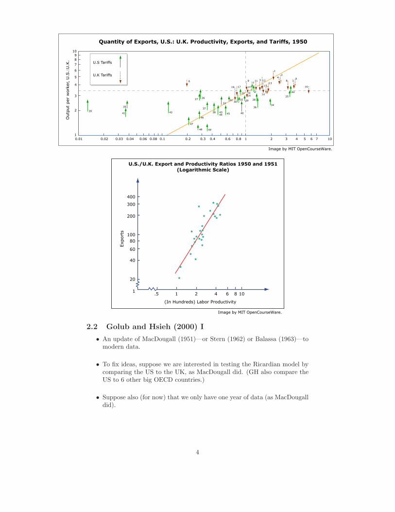
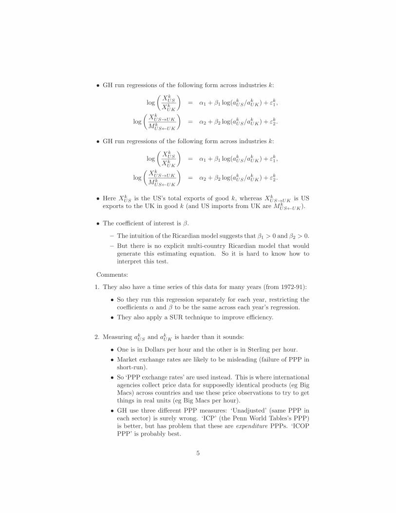
2.2 Golub and Hsieh (2000) I

• An update of MacDougall (1951)—or Stern (1962) or Balassa (1963)—to modern data.

• To fix ideas, suppose we are interested in testing the Ricardian model by comparing the US to the UK, as MacDougall did. (GH also compare the US to 6 other big OECD countries.)

• Suppose also (for now) that we only have one year of data (as MacDougall did).

4

13

42

12

1

2420 21

9

14

1011 3

15

18

1076543210.01 0.02 0.03 0.04 0.06 0.08 0.1 0.2 0.3 0.4 0.6 0.8 1

U.S Tariffs

U.K Tariffs

39

35

41 42

27

6

47

48

46

37

26

19 17

23

38

3331

4344 45

49

40

3032 29 28

3634

25

22

16

578

Quantity of Exports, U.S.: U.K. Productivity, Exports, and Tariffs, 1950

Outp

ut

per

work

er,

U.S

.:U

.K.

2

3

4

5

6

7

89

10

1086421.51

20

40

60

80100

200

300

400

(In Hundreds) Labor Productivity

Exp

ort

s

U.S./U.K. Export and Productivity Ratios 1950 and 1951(Logarithmic Scale)

Image by MIT OpenCourseWare.

Image by MIT OpenCourseWare.

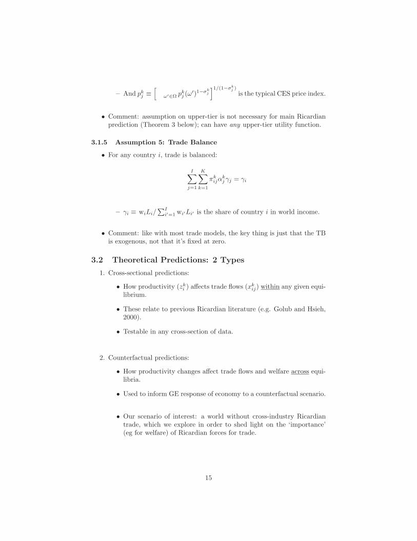
• GH run regressions of the following form across industries k: Xk

US klog = α1 + β1 log(aUS/ak

1 ,UK) + εk

Xk UK

Xk US→UK klog = α2 + β2 log(aUS/a

k 2 .UK) + εk

Mk US←UK

• GH run regressions of the following form across industries k: Xk

US k klog = α1 + β1 log(aUS/aUK) + εk 1 ,Xk

UK Xk

US→UK k klog = α2 + β2 log(aUS/aUK) + εk 2 . Mk

US←UK

• Here Xk is the US’s total exports of good k, whereas Xk is US US US→UK exports to the UK in good k (and US imports from UK are Mk ).US←UK

• The coefficient of interest is β.

– The intuition of the Ricardian model suggests that β1 > 0 and β2 > 0.

– But there is no explicit multi-country Ricardian model that would generate this estimating equation. So it is hard to know how to interpret this test.

Comments:

1. They also have a time series of this data for many years (from 1972-91):

• So they run this regression separately for each year, restricting the coefficients α and β to be the same across each year’s regression.

• They also apply a SUR technique to improve efficiency.

k k2. Measuring a and a is harder than it sounds: US UK

• One is in Dollars per hour and the other is in Sterling per hour.

• Market exchange rates are likely to be misleading (failure of PPP in short-run).

• So ‘PPP exchange rates’ are used instead. This is where international agencies collect price data for supposedly identical products (eg Big Macs) across countries and use these price observations to try to get things in real units (eg Big Macs per hour).

• GH use three different PPP measures: ‘Unadjusted’ (same PPP in each sector) is surely wrong. ‘ICP’ (the Penn World Tables’s PPP) is better, but has problem that these are expenditure PPPs. ‘ICOP PPP’ is probably best.

5

Discussion of GH (2000) and MacDougall (1951)

• Results in MacDougall (1951) and GH (2000) broadly supportive of Ri­cardian model. But problems remain:

1. Bhagwati (1963): Ricardian theory doesn’t necessarily predict rela­tionships like these.

2. Deardorff (1984): HO model (without FPE) would predict a rela­tionship like this too.

6

US_Japan

US_Germany

US_UK

US_France

US_Italy

US_Canada

US_Australia

84_90

77_91

79_91

78_91

78_91

72_90

81_91

0.33(3.03)3

0.18(4.28)3

0.09(2.78)3

-0.19(-3.50)4

0.36

(5.48)3

0.21(5.29)3

0.16

(2.27)3

0.31(2.96)3

0.15(3.55)3

0.07(2.45)3

-0.24(-3.92)4

0.37

(6.25)3

0.27(6.26)3

0.31

(3.52)3

0.30(2.80)3

0.15(3.80)3

0.23(4.48)3

0.09(1.96)3

0.22

0.08

0.03

0.03

0.09 0.13

0.01

0.04

0.20

0.07

0.02

0.06

0.04

0.10

__

0.18

0.05

0.12

0.03

__

__

__

__

__

Period R2βjk R2βjk R2βjk

Unadjusted ICP PPP ICOP PPP

1Log of US divided by other country exports.2Log of US relative to other productivity.3The coefficient is significant at 1% level with the correct sign.4The coefficient is significant at 1% level with incorrect sign.

Note: log(Xij / Xik ) = αjk1 + βjk1

log(αik / αij )-1 + εijk1 estimated by seemingly unrelated regressions.

t-statistics in parentheses, calculated from heteroskedasticity-consistent (White) standard errors.

Relative exports1 and Relative Productivity2, for 39 Manufacturing Sectors

US-Japan

US-Germany

US-UK

US-France

US-Italy

US-Canada

US-Australia

US-Korea

US-Mexico

84-91

77-90

79-90

78-90

79-89

72-89

81-91

72-90

80-90

0.14(2.07)3

0.46(8.71)3

-0.08(-2.93)4

-0.21

(-7.97)4

0.26

(7.11)3

0.41

(37.44)3

0.72

-0.64

0.46

(5.75)3

(-11.17)4

(6.12)3

-0.12

0.31

(-6.71)4

(4.21)3

0.93

0.56

(36.88)3

(7.50)3

0.20(2.68)3

0.83(17.03)3

-0.02(-1.41)

0.02

(0.52)

0.25

(7.55)3

0.73

(77.15)3

0.89

(7.13)3

0.43(2.99)3

0.07(1.32)

-0.01(-0.06)

0.05

(2.70)3

0.09

0.06

0.03

0.02

0.11 0.01

0.02

0.05

0.02

0.14

0.02

0.10

0.18

0.18

0.10

0.11

0.02

0.02

0.01

0.10

__

0.25

0.05

0.02

0.02

__

__

__

__

__

Period R2bjk R2bjk R2bjk

Unadjusted ICP PPP ICOP PPP

1Log of the ratio of bilateral exports to bilateral imports.2Log of US relative to other productivity.3The coefficient is significant at 1% level with the correct sign.4The coefficient is significant at 1% level with incorrect sign.

Note: log(Xijk / Mijk ) = αjk3 + βjk3

log(aik / aij )-1 + εijk3 estimated by seemingly unrelated regressions.

t-statistics in parentheses, based on heteroskedasticity-consistent (White) standard errors.

Bilateral Trade Balances1 and Relative Productivity2, for 21 Manufacturing Sectors

Image by MIT OpenCourseWare.

Image by MIT OpenCourseWare.

3. Harrigan (2003): Simple partial equilibrium supply-and-demand mod­els predict this relationship too. “A truly GE prediction of Ricardian models is that a productivity advantage in one sector can actually hurt export success in another sector, but GH do not investigate this prediction [and nor has anyone since.]”

4. Harrigan (2003): A test of a trade model needs to have a plausible alternative hypothesis built in which can be explicitly tested (and perhaps rejected).

• Subsequent work (which we will discuss shortly) has tackled ‘Problem 1’, but not ‘Problems 2-4.’

2.3 Nunn (2007)

• Open question in Ricardian model: where do labor cost (ie productivity) differences come from?

– Relatedly, in an empirical setting: are we prepared to assume that productivity differences are exogenous with respect to trade flows?

• Nunn (2007) took an innovative take on this problem.

– (But this paper does not try to tackle the fundamental ‘Problems 1-4’ of Ricardian model-based empirical work highlighted above.)

• Nunn (2007) is an influential paper in the ‘Trade and Institutions’ liter­ature (really: How Institutions ⇒ Trade; a separate literature considers the reverse).

– As we saw in the previous lecture, this literature argues that institu­tional differences across countries do not just have aggregate produc­tivity consequences (as in AJR 2001), but may also have differential productivity differences across industries within countries (industries may differ in their ‘institutional intensity’).

– If that is true, institutional differences should generate scope for com­parative advantage, and hence trade.

2.3.1 Set-up

• The key intuition was seen in Lecture 2:

7

– With imperfect contract enforcement (‘bad courts’) input suppliers who make relationship-specific inputs will under-invest ex ante in fear of ex post hold-up.

– This harms productivity. And it is worse in industries that are particularly-dependent on relationship-specific inputs, and in coun­tries with bad courts.

– Suppose further that productivity (in country i and industry k) is the simple product of the ‘relationship-specific input intensity’ of the industry, zk, and the quality of the country’s legal system, Qi.

– Then we have an institutional microfoundation for each country and kindustry’s productivity level: a = zk × Qi.i

2.3.2 Empirical specification

• Based on this logic, Nunn (2007) estimates the following regression, which is similar to Golub and Hseih (2000)’s regression 1:

kln x = αk + αi + β1z kQi + β2hkHi + β3k

kKi + εk i i

• x is total exports and αk and αi are industry and country fixed effects.

– The inclusion of αk is the same thing as taking differences across countries (like the US-UK comparison that GH did) and pooling all of these pairwise comparisons.

• While the regressor of interest is zkQi, Nunn controls for Heckscher­Ohlin-style effects by including an interaction between industry-level skill-intensity (hk) and country-level skill endowments (Hi), and similarly for capital.

2.3.3 Is this regression justified by theory?

• Nunn appeals to Romalis (AER, 2004) which derived an expression like this from theory.

– Romalis (2004) is a Heckscher-Ohlin model with monopolistic com­petition and trade costs, so FPE is broken.

– One problem with that is that Romalis doesn’t explicitly have ‘tech­nology’ terms (like zkQi) in his regression, though Morrow (2008) derives a version with these included.

8

– A second problem with this appeal to Romalis (2004) is that the model is effectively a two-country model, so it’s not clear whether an expression like this holds in a multi-country (and zero trade costs) world.

• Costinot (2009) provides a justification for the regression if the human and physical capital terms are left out.

k k– Note that by assumption, a = zkQi. So a is log supermodular and i i everything in Costinot (2009) applies.

2.3.4 Where is the data on zk and Qi?

k• z (industry-level ‘relationship-specific input intensity’):

– Nunn follows Rajan and Zingales (AER, 1998) and assumes that the US is a ‘model technology’ country. So data from the US can shed light on the innate nature of the technology of making good k, which works (by assumption) in all countries.

k θkRk– Nunn uses z = , where the sum is over all upstream j j neither supplying industries j to industry k

– θk is the share of industry k’s total input choices sourced from in-j dustry j (according to US 1997 Input-Ouptut Table)

– Rk is a classification done by Rauch (1999) of whether good k isneither a good that is neither ‘sold on an organized exchange’ nor ‘reference priced in industry journals’ (ie it is more likely to be relationship-specific.)

• Qi (country-level ‘quality of legal system’):

– Nunn uses standard measures from the World Bank (based on in­vestors’ perceptions of judicial predictability and enforcement of con­tracts).

9

2.3.5 Comments

• Interpreting the results:

– Regression coefficients are standardized, so they can be compared directly with one another. Hence institution-driven comparative ad­vantage appears to explain more of the world than HO CA.

– But the partial R2 in these regressions is very low (3 % of the non-fixed effects variation can be explained by all regressors combined).

10

Least Contract intensive: lowest zirs1

Most Contract intensive: highest zi

rs1

Poultry processing

Flour milling

Petroleum refineries

Wet corn milling

Aluminum sheet, plate and foilmanufacturing

Primary aluminum production

Nitrogenous fertilizer manufacturing

Rice milling

Prim. nonferrous metal excl.copper and alum.

Tobacco stemming and redrying

Other oilseed processing

Other gas extraction

Coffee and tea manufacturing

Fiber, yarn, and thread mills

Synthetic rubber manufacturing

Synthetic dye and pigmentmanufacturing

Plastic material and resinmanufacturing

Phosphatic fertilizer manufacturing

Ferroalloy and related productsmanufacturing

Frozen food manufacturing

Photographic and photocopying equip.manufacturing

Air and gas compressor manufacturing

Analytical laboratory instr. manufacturing

Other engine equipment manufacturing

Other electronic component manufacturing

Packaging machinery manufacturing

Book publishers

Breweries

Musical instrument manufacturing

Aircraft engine and engine partsmanufacturing

Electricity and signal testing instr.manufacturing

Telephone apparatus manufacturing

Search, detection, and navig. instr.manufacturing

Broadcast and wireless comm. equip.manufacturing

Aircraft manufacturing

Other computer peripheral equip.manufacturing

Audio and video equip. manufacturing

Electronic computer manufacturing

Heavy duty truck manufacturing

Automobile and light truck manufacturing

.024

.024

.036

.036

.053

.058

.087

.099

.111

.132

.144

.171

.173

.180

.184

.190

.195

.196

.200

.200

.810

.819

.822

.824

.826

.831

.840

.851

.854

.872

.873

.880

.888

.891

.893

.901

.904

.956

.977

.980

The contract intensity measures reported are rounded from seven digits to three digits.

The Twenty Least and Twenty Most Contract Intensive Industries

Industry Descriptionzirs1 Industry Descriptionzi

rs1

Judicial quality interaction: ziQc

Capital interaction: kiKc

Log income x intra-industry trade: iiti ln yc

Log income x input variety: (1 - hii) ln yc

Log income x value added: vai ln yc

Log credit/GDP x capital: kiCRc

Skill interaction: hiHc

R2

Industry fixed effects

Number of observations

Country fixed effects

.289**(.013)

Yes

_ _ _

_ _ _

_ _ _

_ _ _

_ _

_ _

_ _

_

Yes

.72

22,598

.318**(.020)

Yes

Yes

.76

10,976

.326**(.023)

.085**

(.017)

.105**(.031)

Yes

Yes

.76

10,976

.235**(.017)

-.117*

(.047)

(.041).576**

.024

(.033)

.020

(.012)

.446**(.075)

Yes

_

_

Yes

.77

15,737

.296**(.024)

(.017)

.063**

.074(.041)

-.137*

.546**

(.067)

(.056)

-.010

.021

(.049)

(.018)

.522**(.103)

Yes

Yes

.76

10,816

Dependent variable is ln xic. The regressions are estimates of (1). The dependent variable is the natural log of exports in industry i bycountry c to all other countries. In all regressions the measure of contract intensity used is zrs1. Standardized beta coefficients arereported, with robust standard errors in brackets, * and ** indicate significance at the 5 and 1 percent levels.

i

(1) (2) (3) (4) (5)

The Determinants of Comparative Advantage

Image by MIT OpenCourseWare.

Image by MIT OpenCourseWare.

So there is lots more to do on explaining export specialization! (Or the specification was wrong and/or there is big time measurement error.)

• Nunn (2007) pursues a number of nice extensions:

– Worry about endogeneity of Qi so IV for it with legal origin (La Porta et al, 1997/1998).

– Propensity score matching: restrict attention to British and French legal origin countries only. Then do matching on them (to control non-parametrically for observed confounders...but note that match­ing never helps to obviate concerns about omitted variable bias due to unobserved confounders).

2.3.6 Similar Ricardian-style Exercises

• A number of other papers pursue similar empirical set-ups to that in Nunn (2007):

– Cunat-Melitz: industry-level volatility × country-level labor market institutions.

– Costinot (JIE, 2009): industry-level job complexity × country-level human capital.

– Levchenko (ReStud, 2007): industry-level complexity × country-level contracting institutions.

11

Judicial quality interaction: ziQc

Skill interaction: hiHc

British legal origin: ziBc

French legal origin: ziFc

German legal origin: ziGc

Socialist legal origin: ziSc

Capital interaction: kiKc

Full set of control variables

Country fixed effects

Industry fixed effects

Number of observations

R2

F-test

Hausman test (p-value)

Over-id test (p-value)

.289**(.013)

No

Yes

Yes

.72

22,598

First stage IV estimates: Dependent variable is ziQc.

OLS and second stage IV estimates: Dependent variable is ln xic.

.385**(.022)

No

Yes

Yes

.72

22,598

-.295**(.033)

-.405**(.025)

-.072(.045)

-.477**(.035)113.1

.00

.00

.326**(.023)

.085**(.017)

.105**(.031)

No

Yes

Yes

.76

10,976

.539**(.044)

.042*(.019)

.183**(.035)

No

Yes

Yes

.76

10,976

-.210**(.038)

-.304**(.030)

-.072(.051)

74.6

.00

.00

.296**(.024)

.063**(.017)

.074(.041)

Yes

Yes

Yes

.76

10,816

.520**(.046)

.023(.019)

.114**(.043)

Yes

Yes

Yes

.76

10,816

-.215**(.036)

-.298**(.028)

-.088(.049)

60.4

.00

.00

In the second stage standardized beta coefficients are reported, with robust standard errors in brackets. The dependent variable is the natural log of exports in industry i bycountry c to all other countries. In the first stage I report regular coefficients, with robust standard errors clustered at the country level reported in brackets. The dependentvariable is the judicial quality interaction ziQc. The measure of contract intensity used is z rs1. Although all explanatory variables in the second stage are also included in the firststage, to conserve space I do not report the first stage coefficients for these variables. The omitted legal origin category is Scandinavian. Because there are no Socialist legalorigin countries in the smaller samples of columns (3)_(5), the Socialist interaction term does not appear as an instrument in these specifications. The reported F-test is for thenull hypothesis that the coefficients for the interaction terms are jointly equal to zero, * and ** indicate significance at the 5 and 1 percent levels.

i

OLS (1) IV (2) OLS (3) IV (4) OLS (5) IV (6)

IV Estimates Using Legal Origins as Instruments

Image by MIT OpenCourseWare.

3

– Manova (2008): industry-level financial dependence × country-level financial depth.

– Chor (2009): (roughly) all of the above in one regression, plus H-O variables (“The Determinants of Comparative Advantage”).

• Nunn and Trefler (2013) survey the ‘trade and institutions’ literature.

Costinot, Donaldson and Komunjer (2012)

• As we have discussed in previous lecture, EK (2002) leads to closed-form predictions about the total volume of trade, but it remains silent about central Ricardian question: Who produces/exports what to whom, i.e. What is the pattern of trade?

• CDK extend EK (2002) in a number of empirically-relevant dimensions in order to bring the Ricardian model closer to the data:

– Multiple industries:

∗ Now the model says nothing about which varieties within an industry get traded: fundamental EK-style indeterminacy moves ‘down’ a level.

∗ But the model does predict aggregate industry trade flows.

∗ These industry-level aggregate trade flow predictions have a very Ricardian feel. These predictions are the core of the paper.

– Also, an extension that weakens the assumption behind EK 2002’s clever choice of within-industry productivity distribution.

Contribution

• The result goes beyond the preceding Ricardian literature we’ve seen (eg MacDougall (1951), Golub and Hseih (2000), and Nunn (2007)):

– Provides theoretical justification for the regression being run. This not only relaxes the minds of the critics, but also adds clarity: it turns out that (according to the Ricardian model) no one was running the right regression before.

– Model helps us to discuss what might be in the error term and hence whether orthogonality restrictions sound plausible.

– Empirical approach explicitly allows (and attempts to correct) for Deardorff (1984)’s selection problem of unobserved productivities.

12

– Explicit GE model allows proper quantification: How important is Ricardian CA for welfare (given the state of the productivity differ­ences and trade costs in the world we live in)?

3.1 A Ricardian Environment

• Essentially: a multi-industry Eaton and Kortum (2002) model.

• Many countries indexed by i.

• Many goods indexed by k.

– Each comprised of infinite number of varieties, ω.

• One factor (‘labor’):

– Freely mobile across industries but not countries.

– In fixed supply Li.

– Paid wage wi.

3.1.1 Assumption 1: Technology

• Productivity zki (ω) is a random variable drawn independently for each triplet (i, k, ω)

• Drawn from a Frechet distribution F ki (·): −θk

i kiF (z) = exp[− z/z ]

• Where:

ki > 0 is location parameter we refer to as ‘fundamental productiv­– z

ki generates scope for cross-industry Ricardian ity’. Heterogeneity in z

comparative advantage. This ‘level’ of CA is the focus of CDK (2011).

– θ > 1 is intra-industry heteroegeneity. Generates scope for intra-industry Ricardian comparative advantage. This ‘level’ of CA is the focus of EK (2002).

13

3.1.2 Assumption 2: Trade Costs

• Standard iceberg formulation:

– For each unit of good k shipped from country i to country j, only 1/dk

ij ≤ 1 units arrive.

– Normalize dk ii = 1

– Assume: dk ≤ dk · dk il ij jl

3.1.3 Assumption 3: Market Structure

• Perfect competition:

k– In any country j price p (ω) paid by buyers of variety ω of good kj is:

k k pj (ω) = min cij (ω)i

dk k ij wi

– Where c (ω) = is the cost of producing and delivering one unit kij z (ω)i

of this variety from country i to country j.

• Comment: paper also develops case or Bertrand competition.

– This builds on the work of Bernard, Eaton, Jensen and Kortum (2003)

– Here, the price paid is the second -lowest price (but the identity of the seller is the seller with the lowest price).

– This alteration doesn’t change any of the results that follow, because the distribution of markups is fixed in BEJK (2003).

3.1.4 Assumption 4: Preferences

• Cobb-Douglas upper-tier (across goods), CES lower-tier (across varieties within goods):

– Expenditure given by:

k

k

k 1−σj

k k xj (ω) = pj (ω) pj · αj wj Lj

k– Where 0 ≤ αk ≤ 1, σj < 1 + θj

14

]

1/(1−σkj )k kAnd pj ≡ ω/∈Ω pj (ω

l)1−σkj– is the typical CES price index.

• Comment: assumption on upper-tier is not necessary for main Ricardian prediction (Theorem 3 below); can have any upper-tier utility function.

3.1.5 Assumption 5: Trade Balance

• For any country i, trade is balanced:

KI KK πk ij α

kj γj = γi

j=1 k=1

I – γi ≡ wiLi/ is the share of country i in world income. i/=1 wi/ Li/

• Comment: like with most trade models, the key thing is just that the TB is exogenous, not that it’s fixed at zero.

3.2 Theoretical Predictions: 2 Types

1. Cross-sectional predictions:

k k• How productivity (z ) affects trade flows (x ) within any given equi­i ij librium.

• These relate to previous Ricardian literature (e.g. Golub and Hsieh, 2000).

• Testable in any cross-section of data.

2. Counterfactual predictions:

• How productivity changes affect trade flows and welfare across equi­libria.

• Used to inform GE response of economy to a counterfactual scenario.

• Our scenario of interest: a world without cross-industry Ricardian trade, which we explore in order to shed light on the ‘importance’ (eg for welfare) of Ricardian forces for trade.

15

]

∑

3.3 Cross-Sectional Predictions kLemma 1. Suppose that Assumptions A1-A4 hold. Let xij be the value of trade

from i to j in industry k. Then for any importer, j, any pair of exporters, i and i , and any pair of goods, k and k ,

k k k k dkxij xi j zi zi ij di jk

ln = θ ln − θ ln .k k k kx z z dk dk ij xi j i i ij i j

where θ > 0.

• Proof: model delivers a ‘gravity equation’ for trade flows and pair of countries i,j.in each industry k. Take differences twice.

• Difficulty of t

k– ‘Fundamental Productivity’ (zi ) is not observed (except in autarky). k kThis is z = E[z (ω)].i i

k– Instead we can only hope to observe ‘Observed Productivity’, z ≡w i E zk(ω)w Ωk , where Ωk is set of varieties of k that i actually pro-i i i duces.

– This is Deardorff’s (1984) selection problem working at the level of varieties, ω.

• CDK show that: −1/θ k zk πkzi i ii = ·

k k πkzz i i i i

– Intuition: more open economies (lower πiik ’s) are able to avoid using

their low productivity draws by importing these varieties.

– This solves the selection problem, but only by extrapolation due to a functional form assumption.

Theorem 2. Suppose that Assumptions A1-A4 hold. Then for any importer, j, any pair of exporters, i and i , and any pair of goods, k and k ,

πwhere x ij ≡ xij ii.

16

( ) ( )

/

[ ]

k∑(w /z θidk

xkij i )−

kij = · αjwjL− jk

i (w′ i′di′j/zk ) θi′

aking Lemma 1 to data:

xijln

(k ˜ ′xki′j

) (k′

i′

)θ ln

(dkijd

= θ ln˜k kzi z

′

− i′j

),

xk′ijx

k ki j zk

′i z′ i dk

′′ ijd

ki′j

k k k

˜ ˜ ˜ ˜

• Note that (if trade costs take the form dk = ) then this has a very ij dij dkj

similar feel to the standard 2 × 2 Ricardian intuition.

– But standard 2 × 2 Ricardian model doesn’t usually specify trade quantities like Theorem 3 does.

– And the Ricardian model here makes this same 2 × 2 prediction for each export destination j.

• Can also write this in ‘gravity equation’ form:

• This derivation answers a lot of questions implicitly left unanswered in the previous Ricardian literature:

k– Should the dependent variable be x or something else? i

– How do we average over multiple country-pair comparisons (ie what to do with the j’s)?

– How do we interpret the regression structurally (ie, What parameter is being estimated)?

– What fixed effects should be included?

– Should we estimate the relationship in levels, logs, semi-log?

– What is in the error term? (Answer here: the error term is ln dk ij

plus measurement error in trade flows.)

• However, this specification is effectively a gravity equation (which we will see many variants of throughout this course) so this cannot be seen as a test of Ricardo vs some other gravity model.

• In the above specification, note that δij and δjk are fixed-effects. Comments

about these:

– These absorb a bunch of economic variables that are important to kthe model (eg e is in δj

k) but which are unknown to us. This is good j and bad.

k– The good: we don’t have to collect data on the e variables—they j kare perfectly controlled for by δj . (And similarly for other variables

like wages and the price indices.) Even if we did have data on these variables such that we could control for them, they would be endoge­nous and their presence in the regression would bias the results. The fixed effects correct for this endogeneity as well.

– The bad: The usual problem with fixed-effect regressions is that the types of counterfactual statements you can make are much more lim­ited. However, in this instance, because of the particular structure of this model, there are a surprising number of counterfactual state­ments that can be made with fixed effects estimates only.

17

ln xkij = γij + γkj + θ ln zki − θ ln dkij

3.4 An Extension

• A1 (Frechet distributed technologies) is restrictive. However, consider the following alternative environment:

[(i)]

1. Productivites are drawn from any distribution that has a single lo­cation parameter (zki ).

2. Production and trade cost differences are small: ck 1j c . . . c ck

Ij .

3. CES parameters are identical: σkj = σ.

• In this environment, Theorems 3 and 5 hold approximately.

– Furthermore: Frechet is the only such distribution in which Theorems 3 and 5 hold exactly, and in which the CES parameter can vary across countries and industries.

3.5 Data: Productivity

• Well-known challenge of finding productivity data that is comparable across countries and industries

– Problem lies in converting nominal revenues into measures of physical output.

– Need internationally comparable producer price deflators, across coun­tries and sectors (Bernard and Jones, 2001).

• We use what we see to be the best available data for this purpose:

– ‘International Comparisions of Output and Productivity (ICOP) In­dustry Database’ from GGDC (Groningen).

• ICOP data:

– Single cross-section in 1997.

– Data are available from 1970-2007, but only fit for our purposes in 1997, the one year in which they collected comparable producer price data.

– Careful attention to matching producer prices in thousands of prod­uct lines.

– 21 OECD countries: 17 Europe plus Japan, Korea, USA.

18

– 13 (2-digit) manufacturing industries.

• As Bernard, Eaton, Jensen and Kortum (2003) point out, in Ricardian world relative productivity is entirely reflected in relative (inverse) pro­ducer prices.

– This is always true in a Ricardian model (since wages cancel).

• But further impetus here:

– It might be tempting to use measures of ‘real output per worker’ instead as a measure of productivity.

– But statistical agencies rarely observe physical output. Instead they observe revenues (Rk ≡ QkP k) and deflate them by some price index i i i

ki ki

R(P k) to try to construct ‘real output’ (≡i ).

P

ki

kiR /P

wiL P L

– So again wages cancel. In a Ricardian world, statistical agencies’ measures of relative ‘real output per worker’ are just relative inverse producer prices.

ki

ki

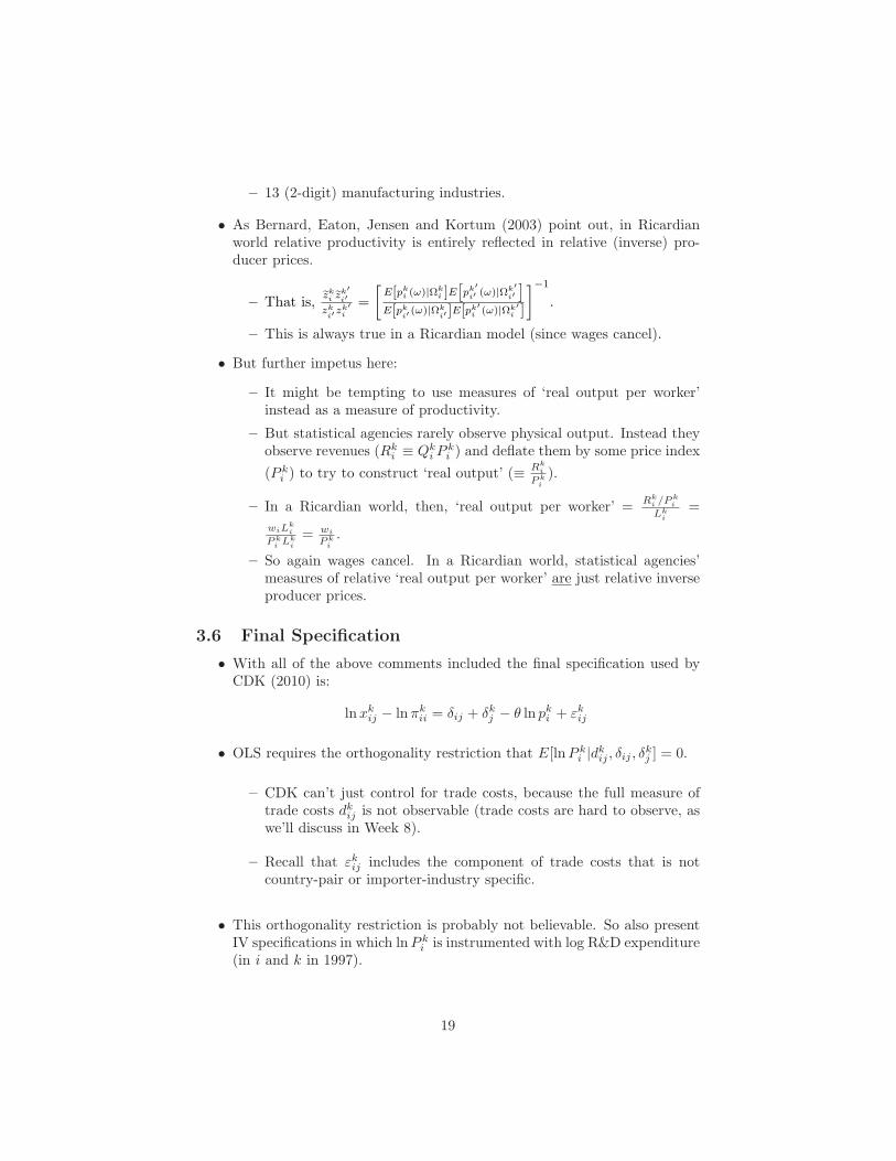
3.6 Final Specification

• With all of the above comments included the final specification used by CDK (2010) is:

k kln xij − ln πk = δij + δjk − θ ln p + εk

ii i ij

• OLS requires the orthogonality restriction that E[ln P k|dk , δij , δk] = 0. i ij j

– CDK can’t just control for trade costs, because the full measure of trade costs dk

ij is not observable (trade costs are hard to observe, as we’ll discuss in Week 8).

– Recall that εk includes the component of trade costs that is not ij country-pair or importer-industry specific.

• This orthogonality restriction is probably not believable. So also present IV specifications in which ln P k is instrumented with log R&D expenditure i (in i and k in 1997).

– In a Ricardian world, then, ‘real output per worker’ = = L

wi= .ki

kiP

ki

19

– That is,zki z

k′i′

zki′z

k′i

=

[E[pki (ω)|Ωk

i ]E[pk

′i′ (ω)|Ωk′

i′

]E[pki′ (ω)|Ωk

i′ ]E[pk′i (ω)|Ωk′

i ]

]−1

.

3.7 Results

log(corrected Dependent variable: log(exports)exports) (1) (2)

log (productivity, 1.123 1.361 based on producer prices) (0.099)*** (0.103)*** Observations 5,652 5,652

R-squared 0.856 0.844

Notes: Regressions include exporter-times-importer fixed effects and importer-times-industry fixed effects. Robust standard errors in parentheses.

Endogeneity Concerns

• Concerns about OLS results:

1. Measurement error in relative observed productivity levels: attenua­tion bias.

2. Simultaneity: act of exporting raises fundamental productivity.

3. OVB: eg endogenous protection (relative trade costs are a function of relative productivity)

• Move to IV analysis:

– Use 1997 R&D expenditure as instrument for productivity (inverse producer prices).

– This follows Eaton and Kortum (2002), and Griffith, Redding and van Reenen (2004).

• Also cut sample: pairs for which dk = dij · dk is more likely. ij j

IV Results

20

log(corrected log(correctedDependent variable: log(exports)exports) exports) (1) (2) (3)

log (productivity, 6.534 11.10 4.621 based on producer prices) (0.708)*** (0.981)*** (0.585)***

Sample Entire Entire EU only Observations 5,576 5,576 2,162

R-squared 0.747 0.460 0.808

Notes: Regressions include exporter-times-importer fixed effects and importer-times-industry fixed effects. Robust standard errors in parentheses.

3.8 Counterfactual Predictions

• Remainder of paper does something different: exploring the model’s re­sponse to counterfactual scenarios.

• CDK’s scenarios aim to answer: How ‘important’ is (cross-industry) Ricar­dian comparative advantage for driving trade flows and gains from trade?

• CDK actually answer a closely related question:

– Suppose that, for any pair of exporters, there were no fundamental relative productivity differences across industries. What would be the consequences of this for aggregate trade flows and welfare?

• More formally:

1. Fix a reference country i0.

2. For all other countries i = i0, assign a new fundamental productivity k k(zi ) ≡ Zi · zi0

.

3. Choose Zi such that terms-of-trade effects on i0 are neutralized: (wi/wi0 ) = (wi/wi0 ).

4. Let Zi0 = 1 (normalization).

5. Refer to all of this as ‘removing country i0’s Ricardian comparative advantage.’

• Questions:

21

6′

′

1. How to compute Zi? (Lemma 4)

2. How to solve for endogenous GE responses under counterfactual sce­nario? (Theorem 5)

3. What model parameters and ingredients (eg trade costs) are needed to answer (a) and (b)?

Lemma 3. Suppose that Assumptions A1-A5 hold. For all countries i = i0, adjustments in absolute productivity, Zi, can be computed as the implicit solution of

−θkKI KK πk zi /Zi αk ij j γj

j=1 k=1 kI πk z /Zi

−θ = γi i =1 i j i

k k(Only need data (πij , z ) and θ. This is a trick first spotted in Dekle, Eaton and i Kortum (2007, IMF paper).)

Theorem 4. Suppose that Assumptions A1-A5 hold. If we remove country i0’s Ricardian comparative advantage, then counterfactual (proportional) changes in

kbilateral trade flows, xij , satisfy

−θkzi /Zi xk = ij I −θkπk z /Zii =1 i j i

k(Again, only need data (πk ) and θ.)ij , zi

Theorem 5. And counterfactual (proportional) changes in country i0’s welfare, kik )−αWi0 ≡ wi0 · (pi0k 0 , satisfy ⎡ ⎤

K IK K zk ⎣ πk iWi0 ii0

−θ kiα 0 /θ

= ⎦

k=1 i=1 zik 0 Zi

We will usually normalize this by the total gains from trade (≡ welfare loss of going to autarky):

ki)−α /θ 0

k=1

3.9 Revealed Productivity Levels k• Counterfactual method requires data on relative zi .

k– Could use data on z from ICOP, but empirics suggest measurement i error is a problem.

– Instead use trade flows to obtain ‘revealed’ productivity:

KKGFTi0 ≡ (πk

i0i0

22

6

( )∑ ( )

∑ ( )

∑ ( )

30

20

30

0

10

20

30

-10

0

10

20

30

Wor

ld

AUS

BEL

CZE

DNK

ESP

FIN

FRA

GER

GRC

HUN

IRE

ITA

JPN

KOR

NDL PO

L

PTL

SVK

USA U

K

USA

-30

-20

-10

0

10

20

30

Wor

ld

AUS

BEL

CZE

DNK

ESP

FIN

FRA

GER

GRC

HUN

IRE

ITA

JPN

KOR

NDL PO

L

PTL

SVK

USA U

K

USA

-50

-40

-30

-20

-10

0

10

20

30

Wor

ld

AUS

BEL

CZE

DNK

ESP

FIN

FRA

GER

GRC

HUN

IRE

ITA

JPN

KOR

NDL PO

L

PTL

SVK

USA U

K

USA

-50

-40

-30

-20

-10

0

10

20

30

Wor

ld

AUS

BEL

CZE

DNK

ESP

FIN

FRA

GER

GRC

HUN

IRE

ITA

JPN

KOR

NDL PO

L

PTL

SVK

USA U

K

USA

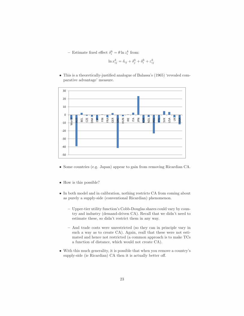
– Estimate fixed effect δik = θ ln zi

k from:

k + εkln x = δij + δjk + δk

ij i ij

• This is a theoretically-justified analogue of Balassa’s (1965) ‘revealed com­parative advantage’ measure.

20

-50

-40

-30

-20

-10

0

10

20

30

Wor

ld

AUS

BEL

CZE

DNK

ESP

FIN

FRA

GER

GRC

HUN

IRE

ITA

JPN

KOR

NDL PO

L

PTL

SVK

USA U

K

USA

• Some countries (e.g. Japan) appear to gain from removing Ricardian CA.

• How is this possible?

• In both model and in calibration, nothing restricts CA from coming about as purely a supply-side (conventional Ricardian) phenomenon.

– Upper-tier utility function’s Cobb-Douglas shares could vary by coun­try and industry (demand-driven CA). Recall that we didn’t need to estimate these, so didn’t restrict them in any way.

– And trade costs were unrestricted (so they can in principle vary in such a way as to create CA). Again, reall that these were not esti­mated and hence not restricted (a common approach is to make TCs a function of distance, which would not create CA).

• With this much generality, it is possible that when you remove a country’s supply-side (ie Ricardian) CA then it is actually better off.

23

4

– Put loosely, this requires that, prior to this change, supply-side and demand/TC-driven CA were offsetting one another. That is, coun­tries prefer (ceteris paribus) the goods that they’re better at produc­ing.

– This ‘offsetting’ sources of CA will mean that autarky prices are actually similar to realized trading equilibrium prices.

• The paper discusses some calibration exercises that confirm this intuition:

– If we restrict tastes to be homogeneous across countries (taking the Cobb-Douglas weights of world expenditure shares), or TCs not to create CA, then fewer countries lose from removing Ricardian CA.

– If we impose both restrictions then no countries lose from removing Ricardian CA.

Rough Ideas for Future Work

• Can one construct a true ‘test’ of the Ricardian model against other models (eg Heckscher-Ohlin, imperfect competition models)?

– Recall Harrigan 1 (2003, Handbook survey): Simple partial equilib­rium supply-and-demand models predict this relationship too. “A truly GE prediction of Ricardian models is that a productivity ad­vantage in one sector can actually hurt export success in another sector.”

– And Harrigan 2 (2003, Handbook survey): A test of a trade model needs to have a plausible alternative hypothesis built in which can be explicitly tested (and perhaps rejected).

• Theoretical papers on the Ricardian model that haven’t (to my knowledge) been explored empirically yet:

– Jones (ReStud, 1961)

– Costinot (Ecta, 2009)

– Wilson (Ecta, 1980)

• How correlated are tastes and technology (and trade costs...and even factor endowments) in the world we inhabit, and how does this feature of reality shape the gains from trade (due to CA) that countries can possibly enjoy?

24

• Are there any ways to get around the Deardorff (1984) selection problem less parametrically than in CDK (2012)?

– Settings in which we actually observe productivities of counterfactual activities? (We will see a bit of this in the next lecture).

– Revealed preference techniques?

– Methods that could bound the behavior of a non-parametric Ricar­dian economy?

25

MIT OpenCourseWarehttp://ocw.mit.edu

14.581International Economics ISpring 2013

For information about citing these materials or our Terms of Use, visit: http://ocw.mit.edu/terms.