145-2013: Know Thy Data: Techniques for Data...

Paper 145-2013

Know Thy Data: Techniques for Data Exploration

Andrew T. Kuligowski, HSNCharu Shankar, SAS Canada

ABSTRACT

Get to know the #1 rule for data specialists: Know thy data. Is it clean? What are the keys? Is it indexed? Whatabout missing data, outliers, and so on? Failure to understand these aspects of your data will result in a flawedreport, forecast, or model.

In this hands-on workshop,

• You will learn multiple ways of looking at data and its characteristics.

• You will learn to leverage PROC MEANS and PROC FREQ to explore your data.

• You will learn how to use PROC CONTENTS and PROC DATASETS to explore attributes and determinewhether indexing is a good idea.

• You will learn to employ powerful PROC SQL’s dictionary tables to easily explore aspects of your data.

INTRODUCTION

Before 1900 the Pima Indians of Arizona were one of the world’s healthiest ethnic groups. Diabetes was unheard of.Things exploded in the 1970s. At 38% and climbing in 2006, the Pima had the highest rate of diabetes of anypopulation in the world. They also had staggering rates of obesity (~70%) and hypertension.

Investigators are interested in examining the occurrence of Type 2 diabetes in women of Pima Indian heritage whoare at least 21 years old.

Using interesting and compelling data of the Pima Indians, follow along in this practical hands-on workshop to learnmultiple data exploration techniques to get to know your data.

Display 1. The population of interest lives in Phoenix, Arizona

1

Hands-on WorkshopsSAS Global Forum 2013

PART 1A: THE SAS® EXPLORER

Display 2. SAS Explorer

The first tool that can be used to learn about a SAS dataset is the Properties window. Actually, that’s not quite true –the first tool is the SAS Explorer window itself! By double-clicking on “Libraries”, you can discover what libraries arecurrently defined to your SAS session. Double-clicking on each of the libraries will show you the SAS datasetscontained within it. Then, you can right-click on an individual dataset to bring up a pop-up menu, with “Properties” asthe final selection of the library. “View Columns” is also a viable option that will provide a limited look at the dataset,focusing on variable names. This same information is available on one of the tabs that will be displayed if“Properties” is selected, in addition to other information on other tabs.

2


computers of that era, a good deal of the information provided in the windows that were discussed earlier wasavailable to the SAS user. PROC CONTENTS would provide information about an individual SAS dataset, whilePROC DATASETS produced information about the entire data library and the datasets it contained.

These two PROCs are still available and still useful today; in fact, additional features have been added to themacross releases since those early days – but since this is not intended as a history lesson, let us review theprocedures as they exist today.

The basic syntax for PROC CONTENTS is quite simple, as parameters and statements are entirely optional. Theoutput, or at least the values displayed in the output, looks remarkably like what was observed in the SAS DatasetProperties window. This aesthetic can be addressed via ODS, which is well outside the scope of this particularpresentation.

The Program Editor window: PROC CONTENTS DATA=<dataset name>;

RUN;

The Output window:The CONTENTS Procedure

Data Set Name ORIGDATA.PIMADEMOGRAPHICS Observations 768

Member Type DATA Variables 4

Engine V9 Indexes 0

Created Thursday, January 31, 2013 02:09:09 PM Observation Length 32

Last Modified Thursday, January 31, 2013 02:09:09 PM Deleted Observations 0

Protection Compressed NO

Data Set Type Sorted NO

Label

Data Representation WINDOWS_64

Encoding wlatin1 Western (Windows)

Engine/Host Dependent Information

Data Set Page Size 4096

Number of Data Set Pages 7

First Data Page 1

Max Obs per Page 126

Obs in First Data Page 83

Number of Data Set Repairs 0

File Name <directory structure redacted>/pimademographics.sas7bdat

Release Created 9.0301M0

Host Created X64_7PRO

Inode Number 150957

Access Permission rw-r--r--

Owner Name <userid redacted>

File Size (bytes) 29696

Alphabetic List of Variables and Attributes

# Variable Type Len

2 Age Num 8

3 Class Num 8

1 Pregnancies Num 8

4 id Char 3

Display 4. PROC CONTENTS example

The example only used one option: DATA=. Even that is technically optional, as SAS will run the procedure on thelast dataset it used if one is not specified. However, it is an elementary Best Practice to always include it wheninvoking a PROC. It can be made more powerful by using DATA=_ALL_, which will display all of the datasets in agiven Data Library.

Other options that can be used to tailor your output are

DIRECTORYPrints a list of all datasets in the specified SAS Data Library.NOPRINT Suppresses the visual output. It technically can be used without the OUT= option, but the result is a

procedure that produces no results whatsoever.

4


OUT= Specifies a SAS dataset which will contain the information displayed in the output table. There willbe one record per variable; information regarding the dataset as an entire entity will beincluded on each record.

OUT2= Specifies a SAS dataset which will contain the information displayed in the output tableSHORT Suppresses the information about the entire dataset, and only displays the data about the individual

variables. Do not use in conjunction with OUT=, or your result will be an empty dataset.VARNUM Lists the variables in the order stored in the dataset, rather than the default of alphabetically.

Please refer to the PROC CONTENTS entry in the SAS PROCEDURES GUIDE for a complete list of options, as wellas non-PROC-specific statements that can be employed in PROC CONTENTS.

PROC DATASETS provides even more power to the SAS user. It is not just that the procedure will work againstevery dataset in the SAS Data Library; after all, with a few well-chosen options, PROC CONTENTS can be made todo that. It’s not even the fact that you can execute multiple commands within one invocation of the PROC, eachseparated by a RUN; statement – QUIT; terminates the entire PROC. After all, the SAS user could do the same thingby simply invoking PROC CONTENTS multiple times. Rather, it is because PROC DATASETS provides the userwith the ability to change selected aspects of a dataset, not simply to display them.

Let’s look at a simple PROC DATASETS request, paralleling what we did earlier via PROC CONTENTS – except,this time, the process will be done on every dataset in the library. Alert readers will notice that the example points toORIGDATA twice, although the second is commented out. This is to remind the reader that some parameters havealiases – in this case, LIBRARY= can also be referred to as DDNAME=. (This is another throwback to the early dayswhen SAS only ran on IBM mainframes.) The password parameters PW= and READ= are also commented out, toshow that they exist, but they are unnecessary since our data library is not password protected.

The CONTENTS statement specifically executes the equivalent of a PROC CONTENTS, while the DATA=_ALL_which was referenced in our discussion of PROC CONTENTS does act upon every dataset in the SAS Data Library.Since we have NOPRINT and OUT=, we will be writing the output to a dataset and not printing anything to theOUTPUT window.

PROC DATASETS DDNAME=ORIGDATA /*** LIBRARY=ORIGDATA ***/

NOLIST NODETAILS

/*** PW= READ= ***/ ;

CONTENTS DATA=_ALL_ OUT=WORK.Original_Datasets NOPRINT NODETAILS DIRECTORY ;

QUIT;

Display 5. PROC DATASETS example

As mentioned, this does not reflect the true power of this procedure; rather, it is the stepping stone to it. Among thethings you use PROC DATASETS for are (referencing specific statements):

APPEND Add the records in one SAS dataset to the bottom of another SAS dataset. This brings the powerof PROC APPEND to this procedure, as well.

CHANGE Allows the user to rename one or more SAS datasets in a SAS Data Library.COPY Copies SAS datasets from one SAS Data Library to another. By default, all datasets are copied;

the selection can be limited via SELECT or EXCLUDE statements.DELETE Removes one or more SAS datasets from a SAS Data Library.EXCHANGE Swaps the names of two SAS datasets within a SAS Data Library.FORMAT Assigns, removes and changes formats assigned to variables in a SAS dataset.INFORMAT Assigns, removes and changes informats assigned to variables in a SAS dataset.MODIFY Allows the alternation of some attributes of a SAS dataset – passwords, for example – and

facilitates the use of other commands to change even more attributes.RENAME= Changes the name of variables within a dataset when used in conjunction with a MODIFY

statement.SAVE Removes all SAS datasets from a SAS Data Library except those specified via this statement.

PART 2: PROC SQL DICTIONARY TABLES

Have you ever wished for more than what PROC CONTENTS can deliver on your metadata? Have you ever rightclicked on a SAS dataset in the SAS explorer window to check properties and wanted more? Have you ever wantedto go behind the scenes and get information on all the titles, macros, datasets, pretty much everything in a session.Well here is your chance to get to know your data through powerful dictionary tables.

5


Dictionary tables contain a wealth of information about your SAS session. They are special read-only PROC SQLtables or views. They are created upon SAS invocation, updated automatically by SAS and are available throughout aSAS session. They provide information about SAS libraries, SAS data sets, SAS system options, and external filesthat are associated with the current SAS session and much, much more.

2.1 Look up dictionary tables easily in SAS

Where do we begin to look up this amazing information? Open up the SASHELP library to view availabledictionary tables:

Display 6. SASHELP views

2.2 Examine Metadata

How do we gather names of all supported tables and views from these powerful tables? Dictionary tables can bequeried using PROC SQL. They can also be accessed by the datastep and other SAS procedures by using thePROC SQL dictionary table views stored in the SASHELP library.

Submit the following code to display all supported dictionary tables and views.

proc sql ;

select distinct memname

from dictionary.dictionaries;

Display 7. Examine metadata

The following table describes available DICTIONARY tables and associated SASHELP views.

DICTIONARY Table SASHELP View Description

CATALOGS VCATALG Contains information about known SAS catalogs.

CHECK_CONSTRAINTS VCHKCON Contains information about known checkconstraints.

COLUMNS VCOLUMN Contains information about columns in all knowntables.

CONSTRAINT_COLUMN_USAGE VCNCOLU Contains information about columns that arereferred to by integrity constraints.

CONSTRAINT_TABLE_USAGE VCNTABU Contains information about tables that haveintegrity constraints defined on them.

DATAITEMS VDATAIT Contains information about known information mapdata items.

6


DESTINATIONS VDEST Contains information about known ODSdestinations.

DICTIONARIES VDCTNRY Contains information about all DICTIONARY tables.

ENGINES VENGINE Contains information about SAS engines.

EXTFILES VEXTFL Contains information about known external files.

FILTERS VFILTER Contains information about known information mapfilters.

FORMATS VFORMAT VCFORMAT

Contains information about currently accessibleformats and informats.

FUNCTIONS VFUNC Contains information about currently accessiblefunctions.

GOPTIONS VGOPT VALLOPT

Contains information about currently definedgraphics options (SAS/GRAPH software).SASHELP.VALLOPT includes SAS system optionsas well as graphics options.

INDEXES VINDEX Contains information about known indexes.

INFOMAPS VINFOMP Contains information about known informationmaps.

LIBNAMES VLIBNAM Contains information about currently defined SASlibraries.

MACROS VMACRO Contains information about currently defined macrovariables.

MEMBERS VMEMBER VSACCESVSCATLGVSLIBVSTABLEVSTABVWVSVIEW

Contains information about all objects that are incurrently defined SAS libraries.SASHELP.VMEMBER contains information for allmember types; the other SASHELP views arespecific to particular member types (such as tablesor views).

OPTIONS VOPTION VALLOPT

Contains information about SAS system options.SASHELP.VALLOPT includes graphics options aswell as SAS system options.

REFERENTIAL_CONSTRAINTS VREFCON Contains information about referential constraints.

REMEMBER VREMEMB Contains information about known remembers.

STYLES VSTYLE Contains information about known ODS styles.

TABLE_CONSTRAINTS VTABCON Contains information about integrity constraints inall known tables.

TABLES VTABLE Contains information about known tables.

TITLES VTITLE Contains information about currently defined titlesand footnotes.

VIEWS VVIEW Contains information about known data views.

Display 8. Dictionary tables and associated SASHELP views

2.3 Investigate common columns for joins

7


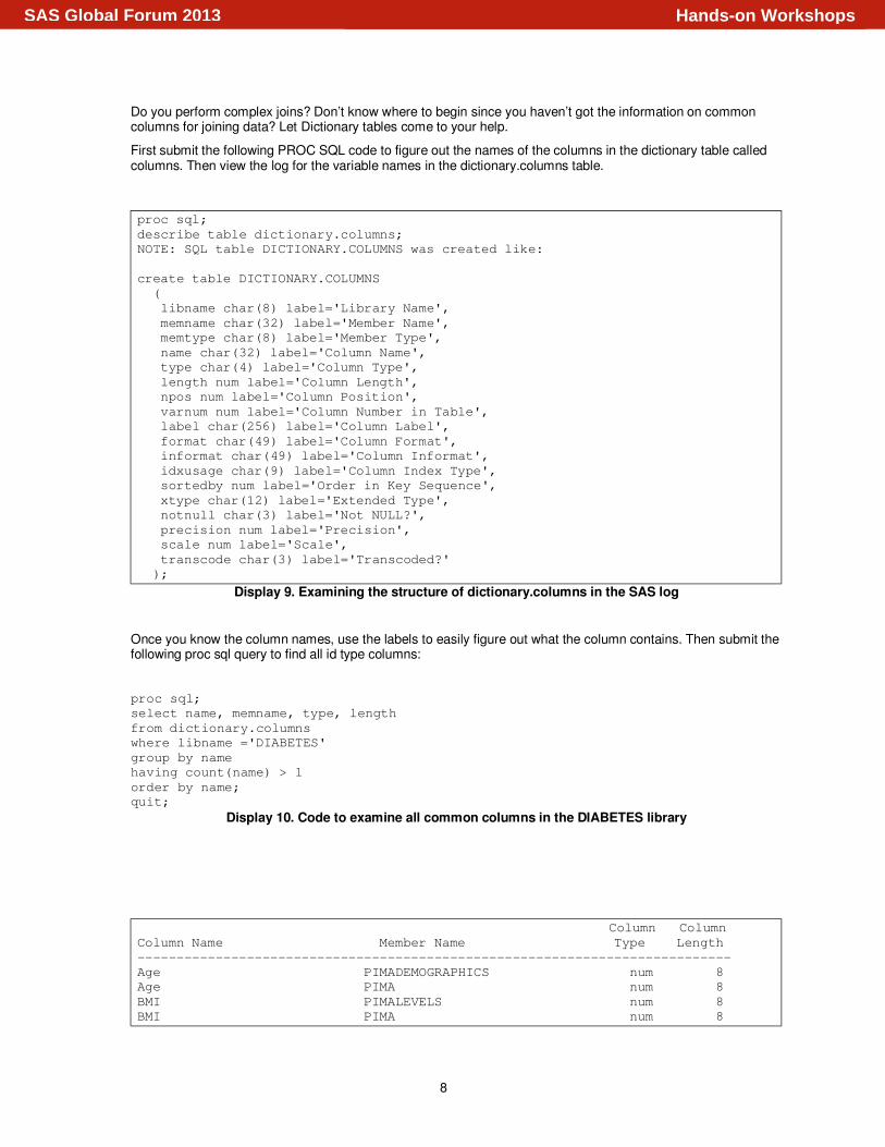
Do you perform complex joins? Don’t know where to begin since you haven’t got the information on commoncolumns for joining data? Let Dictionary tables come to your help.

First submit the following PROC SQL code to figure out the names of the columns in the dictionary table calledcolumns. Then view the log for the variable names in the dictionary.columns table.

proc sql;

describe table dictionary.columns;

NOTE: SQL table DICTIONARY.COLUMNS was created like:

create table DICTIONARY.COLUMNS

(

libname char(8) label='Library Name',

memname char(32) label='Member Name',

memtype char(8) label='Member Type',

name char(32) label='Column Name',

type char(4) label='Column Type',

length num label='Column Length',

npos num label='Column Position',

varnum num label='Column Number in Table',

label char(256) label='Column Label',

format char(49) label='Column Format',

informat char(49) label='Column Informat',

idxusage char(9) label='Column Index Type',

sortedby num label='Order in Key Sequence',

xtype char(12) label='Extended Type',

notnull char(3) label='Not NULL?',

precision num label='Precision',

scale num label='Scale',

transcode char(3) label='Transcoded?'

);

Display 9. Examining the structure of dictionary.columns in the SAS log

Once you know the column names, use the labels to easily figure out what the column contains. Then submit thefollowing proc sql query to find all id type columns:

proc sql;

select name, memname, type, length

from dictionary.columns

where libname ='DIABETES'

group by name

having count(name) > 1

order by name;

quit;

Display 10. Code to examine all common columns in the DIABETES library

Column Column

Column Name Member Name Type Length

----------------------------------------------------------------------------

Age PIMADEMOGRAPHICS num 8

Age PIMA num 8

BMI PIMALEVELS num 8

BMI PIMA num 8

8


Class PIMADEMOGRAPHICS num 8

Class PIMA num 8

DBP PIMALEVELS num 8

DBP PIMA num 8

DiabetesPedigree PIMALEVELS num 8

DiabetesPedigree PIMA num 8

Insulin PIMA num 8

Insulin PIMALEVELS num 8

PlasmaGluc PIMA num 8

PlasmaGluc PIMALEVELS num 8

Pregnancies PIMADEMOGRAPHICS num 8

Pregnancies PIMA num 8

Triceps PIMALEVELS num 8

Triceps PIMA num 8

id PIMA num 8

id PIMALEVELS num 8

id PIMADEMOGRAPHICS char 3

patient_id HISTORY num 8

patient_id VISITS num 8

Display 11. SAS output displays all common columns in the DIABETES dataset

2.4 An efficiency question-PROC SQL or SAS datastep?

Certainly dictionary tables can be accessed either through PROC SQL or SAS procedures/data step code.

options fullstimer;

proc sql;

select libname, memname, name, type, length


where libname ='DIABETES' and name contains 'id';

quit;

NOTE: PROCEDURE SQL used (Total process time):

real time 0.01 seconds

user cpu time 0.00 seconds

system cpu time 0.01 seconds

memory 210.81k

OS Memory 13756.00k

Timestamp 03/14/2013 09:09:59 AM

Display 12. PROC SQL to locate all ID columns in the DIABETES library

If you prefer SAS, use proc print to locate all ID columns in the DIABETES library in your SAS session:

proc print data=sashelp.vcolumn;

var libname memname name type length;

where libname='DIABETES' and name contains 'id';

run;

NOTE: There were 6 observations read from the data set SASHELP.VCOLUMN.

WHERE (libname='DIABETES') and name contains 'id';

NOTE: PROCEDURE PRINT used (Total process time):




memory 1496.39k

OS Memory 14016.00k

Timestamp 03/14/2013 09:10:04 AM

Display 13. Resource usage with PROC PRINT querying dictionary tables in SAS log

9


But, you might be surprised at how much time the SAS step PROC PRINT takes to execute.

Here’s why. While querying a DICTIONARY table, SAS launches a discovery process. Depending on theDICTIONARY table being queried, this discovery process can search libraries, open tables, and execute views.The PROC SQL step runs much faster than other SAS procedures and the DATA step. This is because PROCSQL can optimize the query before the discovery process is launched. It has to do with the processing order. ThePROC SQL step runs much faster because the WHERE clause is processed before the tables referenced by theSASHELP.VCOLUMN view are opened.

Therefore its more efficient to use PROC SQL instead of the DATA Step or SAS procedures to query dictionarytables.

Try it out for yourself. Both programs above produce the same result, BUT….the SAS proc step will probablyhave you wringing your hands as it seems to take forever to execute. By now you know why. It has to searchlibraries, open tables etc. while PROC SQL optimized the query due to the WHERE clause & returns you resultsin a jiffy.

2.5 Locate changed variable names

Date column names have changed and you don’t know what the column names are anymore. Allow Dictionarytables to come to your rescue.

proc sql;

select memname, name, type, length from dictionary.columns

where libname='DIABETES' and upcase(name) like '%DATE%';

quit;

Display 14. Code to query date columns from dictionary.columns table

Column Column

Member Name Column Name Type Length

------------------------------------------------------------------------------------

HISTORY checkupdate num 8

HISTORY followupdate num 8

VISITS date1 num 8

VISITS date2 num 8

Display 15. Output from querying date columns from dictionary.columns table

2.6 Reorder variables in dataset

Data workers frequently request a change in the physical order of variables. Here are their reasons:1. Display PROC PRINT output in alphabetic variable order. Use a variable list shortcut without explicitly

having to type out variable names with the VAR statement.

2. Send SAS output to Excel to help the EXCEL user eliminate manual reordering.

Here’s what happens when you try to use a variable list shortcut. The log complains that variables are out oforder.

proc print data=diabetes.pima;

var dbp--id;

ERROR: Starting variable after ending variable in data set.

run;

NOTE: The SAS System stopped processing this step because of errors.

NOTE: PROCEDURE PRINT used (Total process time):




memory 167.64k

10


OS Memory 14704.00k

Timestamp 03/12/2013 11:14:39 PM

Display 16. Log note when Variable list shortcut for PROC PRINT fails

How are we going to get the variables in order without doing any manual sorting of names & then typing? Let’sutilize a powerful synergy between proc sql and the macro language. We’ll store all the variables from theDIABETES.PIMA dataset in alphabetical order into a macro called newname. This technique uses the INTOclause to pass data values from the dataset into a macro.

proc sql noprint;

select name into :newname separated by ","


where libname ='DIABETES' and

upcase(memname) ='PIMA'

order by name

;

Display 17. Code to put variables in alpha order using dictionary tables

Now read the alphabetically ordered variables just created into a dataset. Voila! No hardcoding required and youhave what you asked for – all variables are stored in alphabetical order.

create table ordered as

select &newname

from diabetes.Pima;

quit;

Display 18. Create table with variables in alpha order

Submit a PROC CONTENTS to verify the order.

proc contents data=ordered;

run;

Display 19. Proc contents to verify variables are in alpha order

Alphabetic List of Variables and Attributes

# Variable Type Len

1 Age Num 8

2 BMI Num 8

3 Class Num 8

4 DBP Num 8

5 DiabetesPedigree Num 8

6 Insulin Num 8

7 PlasmaGluc Num 8

8 Pregnancies Num 8

9 Triceps Num 8

10 id Num 8

Display 20. Neat and tidy variables stored in alpha order, PROC CONTENTS output

2.7 Isolate variable type conflictsHow often have you been stumped with a variable type mismatch while trying to join tables on a common key?Wouldn’t it be more effective to know your data before you start joining? This will help eliminate any surprisesand more importantly conserve time when you have an important deadline to meet.

Gather information on type conflicts by the clever use of the Count function.

proc sql;

select libname, memname, name, type, length


11


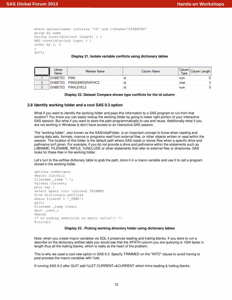
where upcase(name) contains 'ID' and libname='DIABETES'

group by name

having count(distinct length) > 1

AND count(distinct type) > 1

order by 1, 2

;

quit;

Display 21. Isolate variable conflicts using dictionary tables

Display 22. Dataset Compare shows type conflicts for the id column

2.8 Identify working folder and a cool SAS 9.3 option

What if you want to identify the working folder and pass this information to a SAS program to run from thatlocation? You know you can easily lookup the working folder by going to lower right portion of your interactiveSAS session. But what if you want to store the path programmatically to use and reuse. Additionally what if youare not working in Windows & don’t have access to an interactive SAS session.

The "working folder", also known as the SASinitialFolder, is an important concept to know when reading andsaving data sets, formats, macros or programs read from external files, or other objects written or read within thesession. The location of this folder is the default path where SAS reads or stores files when a specific drive andpathname isn't given. For example, if you do not provide a drive and pathname within the statements such asLIBNAME, FILENAME, INFILE, %INCLUDE or other statements that refer to external files or directories, SASlooks for these files in the working folder.

Let’s turn to the extfiles dictionary table to grab the path, store it in a macro variable and use it to call a programstored in the working folder.

options symbolgen;

%macro CurrDir;

filename _temp '.';

%global Current;

proc sql ;

select xpath into :Current TRIMMED

from dictionary.extfiles

where fileref = '_TEMP';

quit;

filename _temp clear;

%put _user_;

%mend;

/* no ending semicolon on macro calls!!! */

%currdir

Display 23 . Picking working directory folder using dictionary tables

Note: when you create macro variables via SQL it preserves leading and trailing blanks. If you were to run adescribe on the dictionary.extfiles table you would see that the XPATH column you are querying is 1024 bytes inlength thus all the trailing blanks, which is really at the heart of the problem.

This is why we used a cool new option in SAS 9.3. Specify TRIMMED on the "INTO" clause to avoid having topost-process the macro variables with %let.

If running SAS 9.2 after QUIT add %LET CURRENT=&CURRENT which trims leading & trailing blanks

12


Now use the macro to call the alloptions.sas program stored in the working directory.

%include "&current\alloptions.sas";

title "Notice no date which was the alloptions program that was being called

by the %include statement";

proc print data=diabetes.pima;

run;

Display 24. Confirming working directory stored in a macro works

Notice no date which was the alloptions program that was being called by the

%include statement

Plasma Diabetes

Obs id Pregnancies Gluc DBP Triceps Insulin BMI Pedigree Age Class

1 1 6 148 72 35 0 33.6 0.627 50 1

2 2 1 85 66 29 0 26.6 0.351 31 0

3 3 8 183 64 0 0 23.3 0.672 32 1

4 4 1 89 66 23 94 28.1 0.167 21 0

5 5 0 137 40 35 168 43.1 2.288 33 1

6 6 5 116 74 0 0 25.6 0.201 30 0

7 7 3 78 50 32 88 31.0 0.248 26 1

8 8 10 115 0 0 0 35.3 0.134 29 0

9 9 2 197 70 45 543 30.5 0.158 53 1

10 10 8 125 96 0 0 0.0 0.232 54 1

Display 25 . PROC PRINT output picks up the alloptions program which set the options to nodate

PART 3: PROCS TO SUMMARIZE DATA

The material discussed to this point discusses file characteristics, field names and their attributes, and methods tolearn about them and to change them. All of these are useful things to know from a programming perspective, butare unlikely to satisfy management’s generic query: “What can you tell me about the data”? (Trust me on this one …)They are more likely to be interested in the values themselves – the row count that we discussed earlier will just whettheir appetite for details about the individual fields and what they actually contain. Fortunately, SAS provides us withnumerous tools to delve into those details of the data.

The first item in our toolkit is PROC MEANS. In its simplest form, PROC MEANS will provide a few basic statistics foreach numeric variable in the specified dataset; these results include defaults Count (N), Mean, and StandardDeviation, with Minimum and Maximum tossed in for good measure – unless overridden. There are several othersavailable upon request, including VAR (variance), STDERR (standard error), NMISS (number missing). and RANGE,In addition, there are several that provide information about quantile (or n-tile if you prefer) points – P1, P5, P10, P25(or Q1), P50 (or MEDIAN), P75 (or Q3), P90, P95, and P99. These are specified via keyword on the OUTPUTstatement.

The default parameter PRINT will cause the PROC to produce a table in the Output window, while NOPRINTsuppresses the table. Of course, in order for the PROC to provide some sort of information, the OUT= parameter onthe OUTPUT statement will write the results to the specified SAS dataset.

The SAS Log window(reflecting the execution of the code in the SAS Program Editor window):759 proc means data=sasglobl.pima;

760 OUTPUT OUT=work.pima_means;

761 run;

NOTE: There were 768 observations read from the data set SASGLOBL.PIMA.

NOTE: The data set WORK.PIMA_MEANS has 5 observations and 13 variables.

NOTE: Compressing data set WORK.PIMA_MEANS increased size by 100.00 percent.

Compressed is 2 pages; un-compressed would require 1 pages.

NOTE: PROCEDURE MEANS used (Total process time):


cpu time 0.04 seconds

The Output window:

13


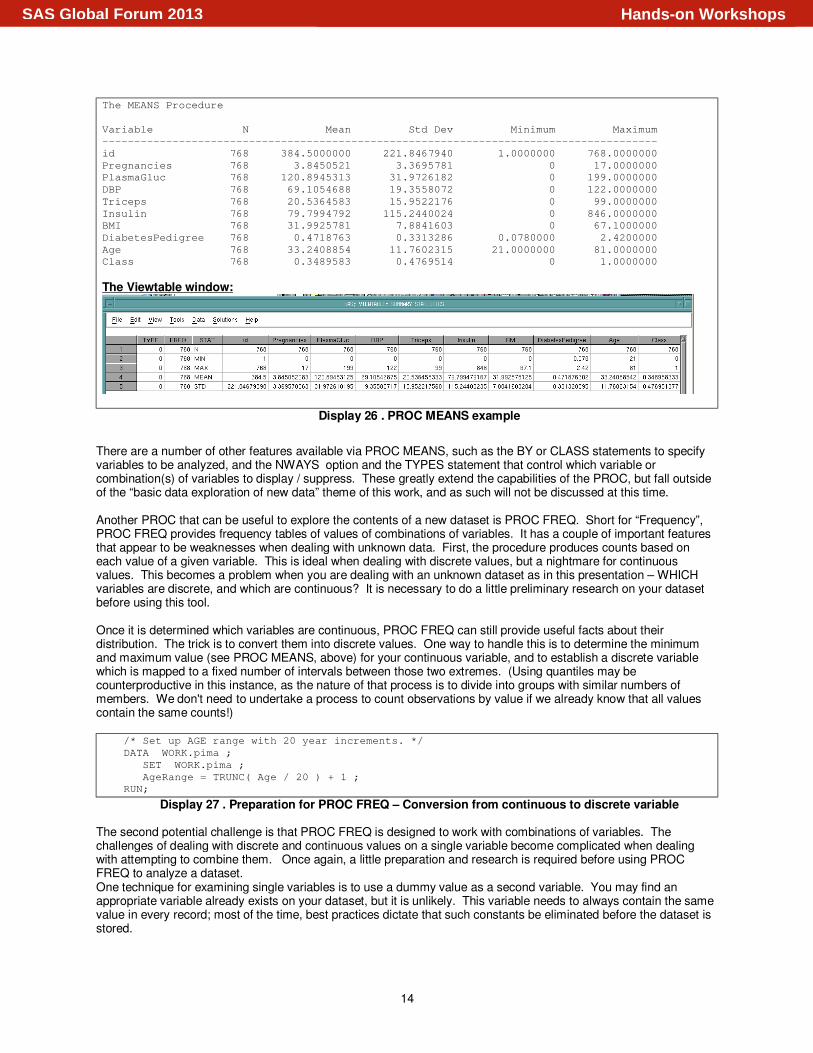
The MEANS Procedure

Variable N Mean Std Dev Minimum Maximum

---------------------------------------------------------------------------------------

id 768 384.5000000 221.8467940 1.0000000 768.0000000

Pregnancies 768 3.8450521 3.3695781 0 17.0000000

PlasmaGluc 768 120.8945313 31.9726182 0 199.0000000

DBP 768 69.1054688 19.3558072 0 122.0000000

Triceps 768 20.5364583 15.9522176 0 99.0000000

Insulin 768 79.7994792 115.2440024 0 846.0000000

BMI 768 31.9925781 7.8841603 0 67.1000000

DiabetesPedigree 768 0.4718763 0.3313286 0.0780000 2.4200000

Age 768 33.2408854 11.7602315 21.0000000 81.0000000

Class 768 0.3489583 0.4769514 0 1.0000000

The Viewtable window:

Display 26 . PROC MEANS example

There are a number of other features available via PROC MEANS, such as the BY or CLASS statements to specifyvariables to be analyzed, and the NWAYS option and the TYPES statement that control which variable orcombination(s) of variables to display / suppress. These greatly extend the capabilities of the PROC, but fall outsideof the “basic data exploration of new data” theme of this work, and as such will not be discussed at this time.

Another PROC that can be useful to explore the contents of a new dataset is PROC FREQ. Short for “Frequency”,PROC FREQ provides frequency tables of values of combinations of variables. It has a couple of important featuresthat appear to be weaknesses when dealing with unknown data. First, the procedure produces counts based oneach value of a given variable. This is ideal when dealing with discrete values, but a nightmare for continuousvalues. This becomes a problem when you are dealing with an unknown dataset as in this presentation – WHICHvariables are discrete, and which are continuous? It is necessary to do a little preliminary research on your datasetbefore using this tool.

Once it is determined which variables are continuous, PROC FREQ can still provide useful facts about theirdistribution. The trick is to convert them into discrete values. One way to handle this is to determine the minimumand maximum value (see PROC MEANS, above) for your continuous variable, and to establish a discrete variablewhich is mapped to a fixed number of intervals between those two extremes. (Using quantiles may becounterproductive in this instance, as the nature of that process is to divide into groups with similar numbers ofmembers. We don't need to undertake a process to count observations by value if we already know that all valuescontain the same counts!)

/* Set up AGE range with 20 year increments. */

DATA WORK.pima ;

SET WORK.pima ;

AgeRange = TRUNC( Age / 20 ) + 1 ;

RUN;

Display 27 . Preparation for PROC FREQ – Conversion from continuous to discrete variable

The second potential challenge is that PROC FREQ is designed to work with combinations of variables. Thechallenges of dealing with discrete and continuous values on a single variable become complicated when dealingwith attempting to combine them. Once again, a little preparation and research is required before using PROCFREQ to analyze a dataset.One technique for examining single variables is to use a dummy value as a second variable. You may find anappropriate variable already exists on your dataset, but it is unlikely. This variable needs to always contain the samevalue in every record; most of the time, best practices dictate that such constants be eliminated before the dataset isstored.

14


/* Set up AGE range with 20 year increments. */

DATA WORK.pima ;

SET WORK.pima ;

RETAIN ExtraVar 1 ;

AgeRange = TRUNC( Age / 20 ) + 1 ;

RUN;

PROC FREQ DATA=WORK.pima ;

TABLES ( Age * ExtraVar / OUT=temp OUTPCT ;

RUN;

Display 28 . Preparation and Invocation of PROC FREQ

The procedure that will provide the greatest amount of information with the least amount of coding or knowledgeabout the data being processed is PROC UNIVARIATE. While PROC MEANS provided 5 facts about each numericvariable, PROC UNIVARIATE provides 5 CATEGORIES of facts for each! Rather than listing them all in thisparagraph, the reader is referred to the accompanying DISPLAY, found immediately below – the listing has beenabbreviated for space considerations, lest it take up half of this paper!

With a few more keystrokes, even more information is available to the data explorer. As with the other PROCs, anOUT= parameter on an OUTPUT statement will allow the results to be stored in a SAS dataset, and a NOPRINT willsuppress the tables from being written to the Output window. Among the more unique options are the HISTOGRAM,PROBPLOT, and QQPLOT statements. These, along with associated options on the PROC statement allowgraphical depictions of the data for those who subscribe to the “picture is worth a 1000 words” approach!

The SAS Log window(reflecting the execution of the code in the SAS Program Editor window):815 proc univariate data=sasglobl.pima;

816 run;

NOTE: PROCEDURE UNIVARIATE used (Total process time):


cpu time 0.07 seconds

The Output window:The UNIVARIATE Procedure

Variable: Pregnancies

Moments

N 768 Sum Weights 768

Mean 3.84505208 Sum Observations 2953

Std Deviation 3.36957806 Variance 11.3540563

Skewness 0.90167398 Kurtosis 0.15921978

Uncorrected SS 20063 Corrected SS 8708.5612

Coeff Variation 87.6341332 Std Error Mean 0.12158918

Basic Statistical Measures

Location Variability

Mean 3.845052 Std Deviation 3.36958

Median 3.000000 Variance 11.35406

Mode 1.000000 Range 17.00000

Interquartile Range 5.00000

Tests for Location: Mu0=0

Test -Statistic- -----p Value------

Student's t t 31.62331 Pr > |t| <.0001

Sign M 328.5 Pr >= |M| <.0001

Signed Rank S 108076.5 Pr >= |S| <.0001

Quantiles (Definition 5)

Quantile Estimate

100% Max 17

99% 13

95% 10

90% 9

75% Q3 6

50% Median 3

15


25% Q1 1

10% 0

5% 0

1% 0

0% Min 0

Extreme Observations

----Lowest---- ----Highest---

Value Obs Value Obs

0 758 13 745

0 754 14 299

0 737 14 456

0 728 15 89

0 714 17 160

The UNIVARIATE Procedure

Variable: Insulin

Moments

N 768 Sum Weights 768

Mean 79.7994792 Sum Observations 61286

Std Deviation 115.244002 Variance 13281.1801

Skewness 2.27225086 Kurtosis 7.21425955

Uncorrected SS 15077256 Corrected SS 10186665.1

Coeff Variation 144.416986 Std Error Mean 4.15850974

Basic Statistical Measures

Location Variability

Mean 79.79948 Std Deviation 115.24400

Median 30.50000 Variance 13281

Mode 0.00000 Range 846.00000

Interquartile Range 127.50000

Tests for Location: Mu0=0

Test -Statistic- -----p Value------

Student's t t 19.18944 Pr > |t| <.0001

Sign M 197 Pr >= |M| <.0001

Signed Rank S 38907.5 Pr >= |S| <.0001

Quantiles (Definition 5)

Quantile Estimate

100% Max 846.0

99% 540.0

95% 293.0

90% 210.0

75% Q3 127.5

50% Median 30.5

25% Q1 0.0

10% 0.0

5% 0.0

1% 0.0

0% Min 0.0

Extreme Observations

----Lowest---- ----Highest---

Value Obs Value Obs

0 768 579 410

0 767 600 585

0 765 680 248

0 763 744 229

0 762 846 14

Display 29 . PROC UNIVARIATE example

Time and space limitations prevent us from a full exploration of these PROCs, each of which could have an entirepaper devoted to them. The reader is encouraged to read the appropriate section of the SAS Procedures Guide forfurther information on each of these PROCs.

16


CONCLUSION

“Know Thy Data” has to be the most important rule – perhaps the only rule – for Data developers. Too often, SASusers ask “We know we should ‘Know Our Data’ – but we don’t. Can SAS help?” Our goal in this hands-on workshopwas to share the many ways in which SAS and PROC SQL can help to get to know your data. Understanding andusing the many SAS procedures shared in this session would go a long way to ensuring data quality and readinessfor analysis. Embracing PROC SQL’s dictionary tables and realizing their ease of use, will provide you that muchneeded data exploration tool. Leverage both SAS and PROC SQL to get to know your data which in turn will go along way towards performing top notch and accurate data analysis.

REFERENCES / ADDITIONAL READING

Cody, Ron. (2007) Learning SAS by Example. Cary, NC: SAS Institute, Inc.

Cody, Ron. (2004) SAS Functions by Example. Cary, NC: SAS Institute, Inc.

Droogendyk, Harry. “QCYour SAS ® and RDBMS Data Using Dictionary Tables”. 18th Annual SouthEast SAS UsersGroup (SESUG) Conference Savannah, GA, September 26 – 28, 2010.http://analytics.ncsu.edu/sesug/2010/BB04.Droogendyk.pdf

Dunn, Toby. “RE: difference between RUN and QUIT” SAS-L posting of 03 April 2007. Available at

http://www.listserv.uga.edu/cgi-bin/wa?A2=ind0704a&L=sas-l&P=25783

Eberhardt, Peter & Brill, Irene. “How Do I Look it Up If I Cannot Spell It: An Introduction to SAS® Dictionary Tables”.SAS® Users Group International SUGI 31 San Francisco Proceedings, March 26-29, 2006.http://www2.sas.com/proceedings/sugi31/259-31.pdf

Go, Imelda C. “Reordering Variables in a SAS® Data Set”. 10th Annual SouthEast SAS Users Group (SESUG)Conference, Savannah, GA, September 22 – 24, 2002. http://analytics.ncsu.edu/sesug/2002/PS12.pdf#navpanes=0

Lafler, Kirk. “Exploring DICTIONARY Tables and Views”. SAS® Users Group International SUGI 30, Philadelphia,PA, April 10-13, 2005. http://www2.sas.com/proceedings/sugi30/070-30.pdf

Lafler, Kirk. (2004) PROC SQL: Beyond the Basics Using SAS. Cary, NC: SAS Institute, Inc.

Libeg, Linda. ”The SAS® Magical Dictionary Tour”. 19th Annual SouthEast SAS Users Group (SESUG) Conference,Alexandria, VA, October 23–25, 2011. http://analytics.ncsu.edu/sesug/2011/BB09.Libeg.pdf

SAS Institute, Inc. Base SAS Procedures Guide, Version 9.1.3 (2007)http://support.sas.com/onlinedoc/913/docMainpage.jsp

SAS Institute, Inc. Base SAS® 9.3 Procedures Guide (2012).http://support.sas.com/documentation/cdl/en/proc/65145/HTML/default/viewer.htm#titlepage.htm

SAS Institute, Inc. SAS Language Reference: Dictionary, Version 9.1.3 (2007)http://support.sas.com/onlinedoc/913/docMainpage.jsp

SAS Institute, Inc. SAS® 9.3 Statements: Reference (2011).http://support.sas.com/documentation/cdl/en/lestmtsref/63323/HTML/default/viewer.htm#p10bvg3wauedhan1qly0hiokirlv.htm

Website Support.sas.com. “How to view DICTIONARY tables”. Available at http://support.sas.com/documentation/cdl/en/lrcon/62955/HTML/default/viewer.htm#a002300185.htm

ACKNOWLEDGMENTS

Andrew is very grateful to section co-chairs Maribeth Johnson and Nancy Brucken for believing that this topic wouldmake a good presentation, and that Charu and I would be good candidates to present it. He also wishes to offerspecial thanks and acknowledgement to Charu Shankar for agreeing to co-author and co-present this material, andfor putting up with his deadline pushing and other assorted nonsense.

Charu is grateful to Andrew for suggesting she co-author this paper. She appreciates her manager Stephen Keelanand SAS Canada for the support and encouragement to share her SAS and SQL knowledge. She is grateful to hermany wonderful customers and students whose ongoing questions provided the impetus to research & sharedictionary table techniques. Special thanks to section co-chairs Maribeth Johnson and Nancy Brucken for inviting herto present this hands-on workshop at SAS Global Forum.

17


CONTACT INFORMATION

The authors welcome correspondence about this work. You can contact them at:

Andrew T. [email protected]

Charu ShankarSAS Institute Inc.280 King Street EastToronto, ON M5A [email protected]

SAS and all other SAS Institute Inc. product or service names are registered trademarks or trademarks of SASInstitute Inc. in the USA and other countries. ® indicates USA registration.

Other brand and product names are trademarks of their respective companies.

18


APPENDIX

Once the paper was proposed and accepted, the first tangible step towards completion was the creation of test data,with the intent to base all examples off of this standard set of data. To this end, Charu generated 4 SAS datasets andsent them to Andrew via email.

Andrew received an unexpected surprise – are there any other kind? - when he attempted to bring the data up inSAS. Charu generated the data under Windows using SAS 9.3, while Andrew was using a Unix box that at the timewas still on SAS 9.1.3. The second surprise was that it really didn't matter; he could read the data as sent, withouthaving to have Charu resend the data in a mutually acceptable format, such as a SAS Transport file or a CSV file.There was one caveat: SAS provided the following warning in the SASLOG:

NOTE: Data file ORIGDATA.PIMA.DATA is in a format native to another host or the

file encoding does not match the session encoding. Cross Environment Data Access

will be used, which may require additional CPU resources and reduce performance.

A simple PROC COPY did not resolve the situation – the new copies were exact copies of the original datasets,including host-specific information.

In keeping with theme of this presentation, Andrew set out to use the tools that would be discussed to resolve theproblem, and came up with the following generic routine that could handle this situation, as well as any similarsituations in the future.

libname ORIGDATA "<directory redacted>/Samples/HOW/OrigData";

libname SASGLOBL "<directory redacted>/Samples/HOW";

PROC DATASETS DDNAME=ORIGDATA

NOLIST NODETAILS

/*** PW= READ= ***/ ;

CONTENTS DATA=_ALL_ OUT=WORK.Original_Datasets NOPRINT NODETAILS DIRECTORY ;

QUIT;

PROC SORT DATA=Original_Datasets(KEEP=MemName)

OUT=Original_Datasets_Brief NODUPKEY;

BY MemName;

RUN;

%MACRO Duplicate_Em;

DATA _NULL_;

SET Original_Datasets_Brief NOBS=reccnt END=LastRec ;

CALL SYMPUT( "DS_to_Copy" || COMPRESS( PUT( _N_, 5. ) ), MemName );

IF LastRec THEN CALL SYMPUT( "DS_Count", PUT( reccnt, 5. ) );

RUN;

%DO Loop = 1 %TO &DS_Count;

DATA SASGLOBL.&&DS_to_Copy&Loop.. ;

SET ORIGDATA.&&DS_to_Copy&Loop.. ;

RUN;

%END;

%MEND Duplicate_Em;

%Duplicate_Em ;

Shortly after completing the routine and successfully converting all of the datasets to Unix, Andrew discovered thatPROC COPY has a NOCLONE option; among the features not cloned by using this option is "representation ofsource operating system". The original PROC COPY could have solved the problem with the addition of one 7-letterparameter.


145-2013: Know Thy Data: Techniques for Data...

Documents

Transcript of 145-2013: Know Thy Data: Techniques for Data...