Published by

Global Observation Research Initiative in Alpine Environments (GLORIA), Austrian Academy of Sciences & University of Natural Resources and Life Sciences Vienna, Austria,with support of the European Union, MAVA Foundation for Nature Conservation, Consortium for Integrated Research in Western Mountains (CIRMOUNT), Consortium for Sustainable Development of the Andean Ecoregion (CONDESAN), Missouri Botanical Garden, International Centre for Integrated Mountain Development (ICIMOD) and a number of further supporters (see the acknowledgements)

Copyright © GLORIA 2015

Published March 2015

Coordinating authors and editors

Harald Pauli, Michael Gottfried, Andrea Lamprecht, Sophie Niessner, Sabine Rumpf, Manuela Winkler, Klaus Steinbauer & Georg Grabherr

Layout

Branko Bily

ISBN 978-92-79-45694-7 (electronic) doi 10.2777/095439

Note

The opinions expressed are those of the author(s) only and should not be considered as representative of the official position of the European Commission nor of any of the other supporters.This publication may be downloaded and / or reproduced only for personal research or educational purposes. Reproduction is authorised provided the source is acknowledged.

Citation

Pauli, H.; Gottfried, M.; Lamprecht, A.; Niessner, S.; Rumpf, S.; Winkler, M.; Steinbauer, K. and Grabherr, G., coordinating authors and editors (2015). The GLORIA field manual – standard Multi-Summit approach, supplementary methods and extra approaches. 5th edition. GLORIA-Coordination, Austrian Academy of Sciences & University of Natural Resources and Life Sciences, Vienna.

GLO

BA

L OBSERVATION RESEA

RC

H IN

ITIA

TIV

E IN

ALP

INE ENVIRONMENTS

GLORIA

THE GLORIA* FIELD MANUALSTANDARD MULTI-SUMMIT APPROACH,

SUPPLEMENTARY METHODS AND EXTRA APPROACHES

5TH EDITION

*Global Observation Research Initiative in Alpine Environments

| 7GLORIA FIELD MANUAL – 5TH  EDITION

THE GLORIA* FIELD MANUAL

STANDARD MULTI-SUMMIT APPROACH, SUPPLEMENTARY METHODS AND EXTRA APPROACHES

*Global Observation Research Initiative in Alpine Environments

COORDINATING AUTHORS AND EDITORSHarald Pauli, Michael Gottfried, Andrea Lamprecht, Sophie Niessner, Sabine Rumpf, Manuela Winkler, Klaus Steinbauer & Georg Grabherr

GLORIA COORDINATIONInstitute for Interdisciplinary Mountain Research, Austrian Academy of Sciences & Center for Global Change and Sustainability, University of Natural Resources and Life Sciences, Vienna

Silbergasse 30/ 3, A-1190 Vienna, AustriaEmail: office@gloria.ac.atw w w. g l o r i a . a c . a t

CONTRIBUTING AUTHORS1

Otari Abdaladze (Tbilisi, GE), Nikolay Aguirre (Loja, EC), Maia Akhalkatsi (Tbilisi, GE), Martha Apple (Butte, Montana, US), Igor Artemov (Novosibirsk, RU), Peter Barancok (Bratislava, SK), Adelia Barber (Santa Cruz, California, US), Stephan Beck (La Paz, BO), Lindsey E Bengtson (West Glacier, Montana, US), José Luis Benito Alonso (Jaca, ES), Catie Bishop (Oroville, California, US), Jim Bishop (Oroville, California, US), William Bowman (Boulder, Colorado, US), Julieta Carilla (Tucumán, AR), Philippe Choler (Grenoble, FR), Gheorghe Coldea (Cluj-Napoca, RO), Francisco Cuesta (Quito, EC), Sangay Dema (Lamegonpa, BT), Ann Dennis (Albany, California, US), Jan Dick (Edinburgh, UK), Katharine Dickinson (Dunedin, NZ), Abdeltif El Ouahrani (Tetouan, MA), Brigitta Erschbamer (Innsbruck, AT), Siegrun Ertl (Vienna, AT), Daniel B. Fagre (West Glacier, Montana, US), Fang Zhendong (Zhongdian, Yunnan, CN), Rosa Fernández Calzado (Granada, ES), Anna Maria Fosaa (Torshavn, FO), Helmut Franz (Berchtesgaden, DE), Barbara Friedmann (Vienna, AT), Andreas Futschik (Vienna, AT), Maurizia Gandini (Pavia, IT), Carolina García Lino (La Paz, BO), Rosario G. Gavilán (Madrid, ES), Suresh K. Ghimire (Kathmandu, NP), Dany Ghosn (Chania, GR), Alfredo Grau (Tucumán, AR), Ken Green (Jindabyne, AU), Alba Gutiérrez Girón (Madrid, ES), Stephan Halloy (Santiago, CL), Robbie Hart (Saint Louis, Missouri, US), Starri Heiðmarsson (Akureyri, IS), Dirk Hoffmann (La Paz, BO), Jeff Holmquist (Los Angeles, California, US), Jarle Inge Holten (Trondheim, NO), Ling-Chun Hsieh (Kaohsiung, TW), Jorge Jácome (Bogotá, CO), Juan José Jiménez (Jaca, ES), María Dolores Juri (Chilecito, AR), Róbert Kanka (Bratislava, SK), George Kazakis (Chania, GR), Christian Klettner (Vienna, AT), Jozef Kollár (Bratislava, SK), Ján Krajcí (Bratislava, SK), Per Larsson (Göteborg, SE), María Vanesa Lencinas (Ushuaia, AR), Blanca León (Lima, PE), Ho-Yih Liu (Kaohsiung, TW), Luis Daniel Llambi (Mérida, VE), Luo Peng (Chengdu, Sichuan, CN), Colin Maher (Santa Cruz, California, US), George P. Malanson (Iowa City, Iowa, US), Martin Mallaun (Innsbruck, AT), Alan Mark (Dunedin,

NZ), Rosa Isela Meneses (La Paz, BO), Abderrahmane Merzouki (Tetouan, MA), Ottar Michelsen (Trondheim, NO), Yuri Mikhailov (Yekaterinburg, RU), Constance I. Millar (Albany, California, US), Andrea Mochet Mammoliti (Aosta, IT), Dmitry Moiseev (Yekaterinburg, RU), Pavel Moiseev (Yekaterinburg, RU), Ulf Molau (Göteborg, SE), Joaquín Molero Mesa (Granada, ES), Bob Moseley (Peoria, Illinois, US), Renée B. Mullen (Congerville, Illinois, US), Priscilla Muriel (Quito, EC), Mariana Musicante (Chilecito, AR), Laszlo Nagy (Campinas, BR), George Nakhutsrishvili (Tbilisi, GE), Jalil Noroozi (Tabriz, IR), Panagiotis Nyktas (Chania, GR), Yousuke Obana (Matsumoto, JP), Laura O’Gan (Grand Junction, Colorado, US), Gilberto Parolo (Pavia, IT), Giovanni Pelino (Sulmona, IT), Catherine Pickering (Southport, AU), Mihai Puscas (Cluj-Napoca, RO), Karl Reiter (Vienna, AT), Hlektra Remoundou (Chania, GR), Christian Rixen (Davos, CH), Graziano Rossi (Pavia, IT), Jan Salick (Saint Louis, Missouri, US), Thomas Scheurer (Bern, CH), Teresa Schwarzkopf (Mérida, VE), Anton Seimon (New York, US), Tracie Seimon (New York, US), Stepan Shiyatov (Yekaterinburg, RU), John Smiley (Bishop, California, US), Angela Stanisci (Isernia, IT), Kristina Swerhun (Victoria, British Columbia, CA), Anne Syverhuset (Trondheim, NO), Jean-Paul Theurillat (Champex, CH), Marcello Tomaselli (Parma, IT), Peter Unterluggauer (Innsbruck, AT), Susanna Venn (Melbourne, AU), Luis Villar (Jaca, ES), Pascal Vittoz (Lausanne, CH), Michael Vogel (Berchtesgaden, DE), Gian-Reto Walther (Bern, CH), Sølvi Wehn (Trondheim, NO), Sonja Wipf (Davos, CH), Karina Yager (Greenbelt, Maryland, US), Tatjana Yashina (Ust Koksa, Altai, RU)

1 | Participation in the discussion process for developing the GLORIA standard methods and/or writing parts of the manual of additional activities of GLORIA

8 | GLORIA FIELD MANUAL – 5TH  EDITIONCONTENTS

Preface  11 Acknowledgements  12

1 Introduction  141.1 Climate change and the alpine life zone*  141.2 Objectives and aims  151.3 Stating the role of GLORIA  161.4 Why focus on high mountain environments?  171.5 Vascular plants as target organism group  181.6 Why mountain summit areas as reference units?  191.7 How to start a GLORIA target region  20

2 The GLORIA site selection for the Multi-Summit Approach  212.1 The target region  212.2 Summit selection  212.2.1 The elevation gradient  212.2.2 Considerations and criteria for the summit selection  24

3 Standard sampling design of the Multi-Summit Approach  273.1 Plot types and design outline  283.2 Materials and preparations  303.3 Setup of the permanent plots  303.3.1 The highest summit point (HSP): determination of the principal reference point  303.3.2 Establishing the 1-m² quadrats in 3 m × 3 m quadrat clusters and the summit area corner points  313.3.3 Establishing the boundary lines of the summit areas and the summit area sections  34

4 Standard recording methods (STAM)  374.1 Recording in the 1-m² quadrats  384.1.1 Visual cover estimation in 1-m² quadrats  384.1.2 Pointing with a grid frame in 1-m² quadrats  414.2 Recording in the summit area sections  414.3 Continuous temperature measurements  434.3.1 Temperature data loggers  434.3.2 Devices currently in use  434.3.3 Preparation of temperature loggers  434.3.4 Positioning of temperature data loggers on GLORIA summits  444.4 The photo documentation  464.5 Removal of plot delimitations and considerations for future reassignments and resurveys  494.6 General information on the target region  49

5 Supplementary sampling designs and recording methods (SUPM)  515.1 Supplementary recording in 1-m² quadrats  525.1.1 Recording of bryophytes and lichens in 1-m² quadrats  525.1.2 Subplot-frequency counts in the 1-m² quadrats  525.1.3 Supplementary 1-m² quadrats at the 10-m level  535.2 Supplementary recording in summit area sections  545.2.1 Recording of bryophytes and lichens in summit area sections  545.2.2 Recording of species cover in summit area sections with Point and Flexible Area (PAF) sampling method  545.3 Line-pointing and species recording in 10 m × 10 m squares  56

CONTENTS

| 9GLORIA FIELD MANUAL – 5TH  EDITIONCONTENTS

5.3.1 Line-pointing of vascular plants in 10 m × 10 m squares  575.3.2 Recording of additional species in 10 m × 10 m squares  58

6 Data handling and management  596.1 The species list  596.2 Data input, data consistency, data storage  606.3 Handling of the photo documentation  616.4 Data property rights and data sharing  62

7 Extra approaches in GLORIA (EXAP)  637.1 GLORIA Downslope Plant Survey  657.2 Invertebrate monitoring on GLORIA summits  707.3 GLORIA-associated arthropod monitoring  727.4 Herpetological monitoring on GLORIA summits  757.5 Soil variability at GLORIA sites  797.6 Socio-economic and cultural aspects in GLORIA regions  817.7 Ethnobotany integrated within GLORIA  86

Glossary of terms used in the manual  89 List of Boxes  96 List of Tables  96 List of Figures  97 References cited  98

ANNEX I: Materials for plot setup and recording  107 ANNEX II: Data sampling forms, PART 1: Sampling forms  113 ANNEX II: Data sampling forms, PART 2: Example sheets  124 ANNEX III: Coding of the photo documentation  136

* Terms in italics are explained in the glossary

10 | GLORIA FIELD MANUAL – 5TH  EDITION

| 11GLORIA FIELD MANUAL – 5TH  EDITIONPREFACE

GLORIA, the “Global Observation Research Initiative in Alpine Environments”, is a long-term observation programme and a rapidly growing international research network to assess climate change impacts on the biological richness of the planet’s high mountain ecosystems. A widely applied sampling design, such as the Multi-Summit Approach described here, is an essential prerequisite for collecting comparable data from different mountain regions around the world.

This publication is the fifth and fully revised edition of the GLORIA field manual. The manual contains the detailed description of GLORIA’s basic and standardised sampling design, the Multi-Summit Approach, with complete guidelines of the required procedure from site selection, setup and recording to data compilation. Moreover, it includes supplementary optional methods and a description of additional activities that are ongoing or have been recently initiated in the frame of GLORIA. The field manual represents the technical description of GLORIA approaches; it does not include considerations on data analysis or on how to report the results to the scientific community and to the public.

The introductory chapter 1 of the manual outlines the rationale for an international observation network for ecological and biogeographical climate impact research in mountain regions. Chapter 2 focuses on selection criteria for mountain regions and sites. Chapter 3 describes in detail the standardised design and setup procedure of the Multi-Summit Approach, chapter 4 the recording methods. Distinct consecutive  WORK STEPS  run across chapters 3 and 4 in alphabetic numbers from  A  to  V . Chapter 5 contains descriptions of supplementary optional methods that may be applied within GLORIA summit sites and chapter 6 deals with data input, handling and management. Chapter  7 depicts ongoing additional activities in GLORIA target regions, either focusing on animal organism groups, on transects along mountain slopes, soil studies, on traditional knowledge or on socio-economic changes in GLORIA regions. Boxes provide additional background information throughout. Special terms used in this manual are written in italics and are explained in the glossary.

The previous, 4th edition of the field manual was based on the first Europe-wide field application as part of the GLORIA-EUROPE project of the 5th RTD Framework Programme of the European Union but also involved scientists from other continents. It was published by the Office for Official Publications of the European Communities in 2004 and translated into Spanish and Chinese.

Since then, the number of GLORIA sites has increased almost sixfold with active observation sites in now around

120 study regions (target regions) in mountain systems distributed over six continents. The current 5th edition of the field manual accounts for this change from an initially mainly Europe-based to a world-wide network. The standard Multi-Summit Approach was revised in the view of its global applicability and, further, this new manual was extended to additional GLORIA-related activities, which already have started in several GLORIA regions. This revised manual is based on thorough discussions and agreements met at the GLORIA conference in Perth/Scotland in September 2010, which was attended by participants from 34 countries from all continents.

The full list of existing GLORIA target regions is displayed on the GLORIA website: www.gloria.ac.at. Before starting with the setup of new GLORIA sites (target regions), please, see the website for possible changes and we very much recommend to contact the GLORIA coordination prior to establishing a new site.

Many thanks to all colleagues who have contributed to the build-up of the GLORIA long-term observation network and the development, revision and extension of this field manual. All the best for your upcoming mountain fieldwork.

The GLORIA coordination Vienna, June 2014

PREFACE

GLORIA FIELD MANUAL – 5TH  EDITIONACKNOWLEDGEMENTS12 |

We wish to thank all who have supported and contributed to the development of the international GLORIA network and research programme since the stimulating initiating discussions of the Multi-Summit Approach at the Conference on Environmental and Societal Change in Mountain Regions (Oxford 1997) and the inauguration conference of the Global Mountain Biodiversity Assessment (GMBA, Rigi/Switzerland, 2000).

We acknowledge a range of different financial supporters. Important supporting institutions in the beginning test and development phase were the Austrian Academy of Sciences (ÖAW) through a contribution to the International Geosphere-Biosphere Programme (IGBP), the University of Vienna and the Austrian Federal Ministry of Education, Science and Culture. GLORIA’s implementation phase commenced through the European Union’s 5th RTD framework programme with the pan-European project GLORIA-Europe (EVK2-CT-2000-0056; European Commission officers Alan Cross and Riccardo Casale). Alan Cross’ starting statement in 2001 “this project has an enormous potential” can now, a decade after this project ended, be seen as well fulfilled in the view of a sixfold extension of this now global programme. The world-wide extension and resurvey activities were supported through several inter-governmental institutions, such as UNESCO’s MaB programme, the European Environment Agency (EEA)/European Topic Centre on Biological Diversity, the European Union’s 6th RTD framework programme, the Andean Environmental Agenda of the Comunidad Andina (CAN), the Swiss Development Cooperation/Andes Programme, and the International Centre for Integrated Mountain Development of the Hindu Kush-Himalaya region (ICIMOD). National funding was provided in many countries for the setup of GLORIA sites. Among the important supporters were also private foundations and organisations such as the Swiss MAVA-Foundation for Nature Conservation, the National Geographic Society, the Wildlife Conservation Society, NGOs like The Nature Conservancy, Conservation International and a large number of research institutions and consortia including CONDESAN, Missouri Botanical Garden, and CIRMOUNT.

The GLORIA coordination is affiliated with the Institute for Interdisciplinary Mountain Research at the Austrian Academy of Science (ÖAW) and the Center for Global Change and Sustainability at the University of Natural Resources and Life Sciences (BOKU), Vienna, and was supported by the Austrian Federal Ministries BMWF, BMLFUW, the government of Tyrol, and the Swiss MAVA foundation; the latter also provided

particular funding for this revised version of the field manual.

As the majority of GLORIA sites are situated within protected areas, a continued support through and cooperation with conservation management authorities of national parks, UNESCO Biosphere Reserves and regional protected areas is particularly thankworthy.

The development, implementation and maintenance would not have been possible without the sustained commitment of the large number of devoted biologists, mountain geographers, and conservationists who provided advice, contributed to earlier versions of the GLORIA field manual, were acting as communicators, supporters, supervisors of field surveys, and/or were doing alpine field work (around 500 persons were involved in the frame of GLORIA), data compilation and data analysis.

In this respect, we greatly acknowledge the efforts of: Clemens Abs (Berchtesgaden, DE), Manuel Alcántara (Zaragoza, ES), Patricio Andino (Quito, EC), Jaroslav Andrle (Vrchlabi, CZ), Kerstin Anschlag (Bonn, DE), Marco Arenas Aspilcueta (Huaraz, PE), Kevin Arseneau (Moncton, New Brunswick, CA), Alberto Arzak (Bilbao, ES), Isabel W. Ashton (Fort Collins, Colorado, US), Serge Aubert (Grenoble, FR), Svetlana Babina (Kuznetskiy Alatau BR, RU), Selene Báez (Quito, EC), Barry Baker (Fort Collins, Colorado, US), Gretchen Baker (Baker, Nevada, US), Christian Bay (Copenhagen, DK), Neil Bayfield (Glassel, UK), María Teresa Becerra (Bogotá, CO), Valeria Becette (Chilecito, AR), Andreas Beiser (Feldkirch, AT), Rosita Soto Benavides (Copiapó, CL), Elizabeth Bergstrom (Nevada, US), Tomas Bergström (Östersund, SE), Jean-Luc Borel (Grenoble, FR), Phyllis Pineda Bovin (Fort Collins, Colorado, US), Maurizio Bovio (Aosta, IT), Frank Breiner (Bayreuth, DE), Stanislav Brezina (Vrchlabi, CZ), Michael Britten (Fort Collins, Colorado, US), Álvaro Bueno Sánchez (Oviedo, ES), Harald Bugmann (Zurich, CH), Ramona J. Butz (La Merced, California, US), Matilde Cabrera (Zaragoza, ES), Martin Camenisch (Chur, CH), Rolando Céspedes (La Paz, BO), Gustavo Chacón (Cuenca, EC), Ram Prasad Chaudhari (Kathmandu, NP), Nakul Chettri (Kathmandu, NP), Svetlana Chukhontseva (Altaiskiy BR, RU), Jane Cipra (Death Valley, California, US), Pierre Commenville (Nice, FR), Craig Conely (Las Vegas, New Mexico, US), Emmanuel Corcket (Grenoble, FR), Marco Cortes (Temuco, CL), Julie Crawford (Silverton, Colorado, US), Ana Soledad Cuello (Tucumán, AR), Susie Dain-Owens (Salt Lake City, Utah, US), Evgeny A. Davydov (Barnaul, Altai, RU), Thomas Dirnböck (Vienna, AT), Jiri Dolezal (Třeboň, CZ),

ACKNOWLEDGEMENTS

ACKNOWLEDGEMENTS | 13GLORIA FIELD MANUAL – 5TH  EDITION

Pablo Dourojeanni (Huaraz, PE), Fabian Drenkhan (Lima, PE), Stefan Dullinger (Vienna, AT), Miroslav Dvorský (Ceske Budejovice, CZ), Paul Alexander Eguiguren (Loja, EC), Rodrigo Espinosa (Quito, EC), Angie Evenden (Berkley, California, US), George Fayvush (Yerevan, AM), José Ignacio Alonso Felpete (Oviedo, ES), Miltón Fernández (Cochabamba, BO), Thomas Fickert (Passau, DE), Anton Fischer (Freising, DE), Guillaume Fortin (Moncton, New Brunswick, CA), Andrés Fuentes Ramírez (Temuco, CL), Zaira Gallardo (Piura, PE), Luis Enrique Gámez (Mérida, VE), Thomas Gassner (Vienna, AT), Carmen Giancola (Isernia, IT), Andreas Goetz (Schaan, LI), Markus Gottfried (Vienna, AT), Ricardo Grau (Tucumán, AR), Greg Greenwood (Berne, CH), Friederike Grüninger (Passau, DE), Matteo Gualmini (Parma, IT), Sylvia Haultain (Three Rivers, California,  US), Kimberly Heinemeyer (Salt Lake City, Utah, US), Andreas Hemp (Bayreuth, DE), Wendy Hill (Southport, AU), Daniela Hohenwallner (Innsbruck, AT), Karen Holzer (West Glacier, Montana, US), Margaret Horner (Baker, Nevada, US), Michael Hoschitz (Vienna, AT), Erick Enrique Hoyos Granda (Piura, PE), Karl Hülber (Vienna,  AT), Hakan Hytteborn (Trondheim, NO), David Inouye (La Merced, California, US), Javier Irazábal (Quito, EC), Zoltan Jablonovszki (Cluj-Napoca, RO), Glen Jamieson (Parksville, British Columbia, CA), Ricardo Jaramillo (Quito, EC), Michael T. Jones (Concord, Massachusetts, US), Janet Jorgenson (Fairbanks, Alaska, US), Mary T. Kalin Arroyo (Santiago, CL), Vladislav Kanzai (Kyzyl, Tuva, RU), Rüdiger Kaufmann (Innsbruck, AT), James B. Kirkpatrick (Hobart, Tasmania, AU), Martin Klipp (Graz, AT), Roksana Knapik (Jelenia Gora, PL), Katie Konchar (Saint Louis, Missouri, US), Christian Körner (Basel,  CH), Daniel Kreiner (Admont, AT), Ditte Katrine Kristensen (Copenhagen, DK), Hörður Kristinsson (Akureyri, IS), Thomas Kudernatsch (Freising, DE), Lara Kueppers (La Merced, California, US), Sonya Laimer (Vienna, AT), Kristin Legg (Bozeman, Montana, US), Benoít Lequette (Saint-Denis, Réunion, FR), Christian Lettner (Vienna, AT), Li Haomin (Kunming, Yunnan,  CN), Javier Loidi Arregui (Bilbao, ES), Kristin Long (Grand Junction, Colorado, US), Jennifer Lyman (Billings, Montana, US), Tania Maegli (Dunedin, NZ), Guillermo Martinez Pastur (Ushuaia, AR), Paul McLaughlin (Fort Collins, Colorado, US), Richard McNeill (Las Vegas, New Mexico, US), Iván Mejía (Piura, PE), Tanja Menegalija (Bled, SI), Bruno Messerli (Bern, CH), Pascale Michel (Dunedin, NZ), Michael Miller (Revelstoke, CA), Alain Morand (Nice,

FR), John Morgan (Bundoora, Victoria, AU), Umberto Morra di Cella (Aosta, IT), Kathren Murrell (Davis, US), Ingemar Näslund (Östersund, SE), Alkinoos Nikolaidis (Chania, GR), Koren Nydick (Silverton, Colorado, US), Tatiana Lizbeth Ojeda Luna (Loja, EC), Ramiro Ortega (Cusco, PE), Stu Osbrack (Albany, California, US), Federico G. Osorio (Vancouver, British Columbia, CA), Július Oszlányi (Bratislava, SK), Vasilios Papanastasis (Thessaloniki, GR), Chelsy Passmore (Anchorage, Alaska, US), Imogen Pearce (Banchory, UK), Baard Pedersen (Trondheim, NO), Pablo Peri (Rio Gallegos, Argentina), Martina Petey (Aosta, IT), Martin Price (Perth, UK), Francisco Prieto (Quito, EC), Martin Prinz (Vienna, AT), Daniel Pritchett (Bishop, California, US), Gopal S. Rawat (Kathmandu, NP), Mel Reasoner (Kamloops, British Columbia, CA), Michael Richter (Erlangen, DE), Nanci Ross (Saint Louis, Missouri, US), Natalia Samaniego (Loja, EC), Cyrus Samimi (Bayreuth, DE), Lina Sarmiento (Mérida, VE), Alyona Sashko (Shushenskoe, Krasnoyarskiy Kray, RU), Toshiyuki Sato (Matsumoto, JP), Ken Sato (Sapporo, JP), Norbert Sauberer (Vienna, AT), Stefan Schindler (Vienna, AT), Niels Martin Schmidt (Copenhagen, DK), Jutta Schmidt-Gengenbach (Los Angeles, California, US), Natalie Schulz (Lima, PE), Eklabya Sharma (Kathmandu, NP), Douglas Sheil (Bwindi, UG), Dan Smith (Victoria, British Columbia, CA), Rosina Soler Esteban (Ushuaia, AR), Torstein Solhøy (Bergen, NO), Eva Spehn (Basel, CH), Hermann Stockinger (Vienna, AT), David Suárez (Quito, EC), Michael Suen (Vienna, AT), Stephen S. Talbot (Anchorage, Alaska, US), Natali Thompson Baldiviezo (La Paz, BO), Martín E. Timaná (Lima, PE), Tadeja Trošt Sedej (Ljubljana, SI), Alfredo Tupayachi (Cusco, PE), Linda Turner (Banchory, UK), Nancy Turner (Victoria, British Columbia, CA), Tudor Ursu (Cluj-Napoca, RO), Miriam van Heist (Bwindi, UG), Omar Varela (Chilecito, AR), Maria Isabel Vieira (Bogotá, CO), Ricardo Villanueva (Huaraz, PE), Paolo Villegas (Piura, PE), Paul Viñas (Piura, PE), Ioannis Vogiatzakis (Chania, GR), Monika Wenzl (Sabadell, ES), Robert D. Westfall (Albany, California, US), Lisabeth L. Willey (Amherst, Massachusetts, US), Wu Ning (Chengdu, Sichuan, CN & Kathmandu, NP), Yi Shaoliang (Kathmandu, NP), Alexander Zateev (Ust Koksa, Altai, RU), and many more who were involved in GLORIA fieldwork and may not be mentioned here.

GLORIA FIELD MANUAL – 5TH  EDITION1 – INTRODUCTION14 |

1.1 CLIMATE CHANGE AND THE ALPINE LIFE ZONE

The purpose of GLORIA (Global Observation Research Initiative in Alpine Environments) is to operate a world-wide long-term observation network for the comparative study of climate change impacts on mountain vegetation and its biodiversity (Grabherr et al. 2000, Pauli et al. 2009, Grabherr et al. 2010).

The earth’s biosphere is currently experiencing and will continue to experience rapid climate change (Solomon et al. 2007). Since the mid-twentieth century, greenhouse gases globally contributed to 0.85K of warming at a 5–95% uncertainty of 0.6-1K, where at least 74% (± 12%) of the observed temperature increase since 1950 was caused by human-induced radiative forcing, and less than 26% (± 12%) by unforced internal variability (Huber & Knutti 2012). The last three decades have been progressively warmer than all earlier decades (Hartmann et al. 2013), and the decade 2000-2009 was the warmest in the instrumental record (Arndt et al. 2010). Predictions of global mean surface warming of up to 2.6 to 4.8 °C towards the end of the 21st century, relative to 1986–2005 (Collins et al. 2013), may drastically alter existing biosphere patterns. All ecosystems will experience climate change, but ecosystems of the alpine life zone (i.e. the high mountain environments above the treeline) are considered to be particularly sensitive to warming because they are determined by low temperature conditions (Sala et al. 2000).

Long-term records on the extent of mountain glaciers provide evidence for an ongoing climate warming in high mountain environments across biomes (Price & Barry 1997, Haeberli et al. 2007, Vuille et al. 2008). Direct impacts of temperature and precipitation changes as well as indirect effects (e.g. through changes of permafrost patterns and of disturbance dynamics, shifts in biotic interaction) of climate change will affect biodiversity and may lead to declines or even to the disappearance of a variety of species. Model projections of climate change impacts on plant diversity suggest that mountain regions could be among the most vulnerable (Halloy & Mark 2003, Thuiller et al. 2005). Suitable habitats of many high mountain plant species could be drastically reduced or disappear by the end of the 21st century, particularly where climate warming is combined with decreasing precipitation (Van de Ven et al. 2007, Engler et al. 2011, McCain & Colwell 2011, Tovar et al. 2013). Even if alpine plants do not disappear rapidly from increasingly unsuitable habitats, a growing ‘extinction debt’ will have to be paid later on, after some decades, if plants are unable to adapt to or cope

with changing conditions (Dullinger et al. 2012). Usually light-demanding alpine plants are expected to decline in competition with taller-growing plants in consequence of treeline advances (Devi et al. 2008, Harsch et al. 2009, Feeley et al. 2011), where a net-gain of mountain forests would result in a much larger relative shrinking of alpine land area, given the smaller areal extent of the latter (Körner 2012). The severity of such »extinction scenarios« of alpine plants can only be documented by long-term in situ monitoring. In contrast to meteorology and glaciology, however, long-term observations for detecting the impacts of climate change on alpine ecosystems are scarce and have been based on incidental historical data from a limited number of sites. Among these few exceptions are old records from summit habitats of the Alps dating back to the 19th century and several historically studied sites in the Scandes and the Scottish Mountains. Resurveys of these historic summit sites showed that vascular plants have been established at higher altitudes than recorded earlier (Grabherr et al. 1994, 2001 a, Klanderud & Birks 2003, Britton et al. 2009, Stöckli et al. 2012, Wipf et al. 2013). Walther et al. (2005) showed that an increase in plant species numbers occurred at a faster pace during the recent decades. Thus, it is assumed that an upward migration of plants, induced by anthropogenic climate warming, is already an ongoing and accelerating process. Changes in species’ ranges and their ability to compensate climate change-driven habitat losses, however, are expected to vary greatly among species and responses may be nonlinear, which could lead to sudden range contractions or expansions when climatic tipping points are exceeded (Doak & Morris 2010).

Broad-scale analyses and literature reviews provided ample evidence of ecological impacts of recent climate change, from low-temperature determined terrestrial to tropical marine environments (Walther et al. 2002, Parmesan & Yohe 2003, Root et al. 2003). A meta-analysis over a range of different organism groups showed that the rate of upward shifts was two or three times faster than previously reported (Chen et al. 2011).

Although a pronounced geomorphological hetero-geneity and a resulting variation in microclimatic patterns (Scherrer & Körner 2010) and a large vertical extension in many mountain ranges may provide local refugia (Gottfried et al. 1999, Randin et al. 2009), repeated GLORIA surveys indicate a progressive shrinking of the low-temperature, high-elevation habitats, and a decline of species numbers in some mountain regions. Recent resurveys of European GLORIA sites provided evidence that alpine vegetation experienced an increase of more “thermophilic plants”

1 INTRODUCTION

GLORIA FIELD MANUAL – 5TH  EDITION1 – INTRODUCTION | 15

(warm-demanding species), which usually dwell at lower elevations and/or a concurrent decline of more “cryophilic species” (cold-adapted plant species) occurring at high elevations (Gottfried et al. 2012). This “thermophilisation” of alpine plant communities was observable across the continent (Gottfried et al. 2012), as was a general upward shift of plant species (Pauli et al. 2012). In northern and central Europe, this led to an increase in species numbers during the past decade (Erschbamer et al. 2011, Pauli et al. 2012). A decline in species cover, however, was found at the lower distribution margins of extreme high-altitude species in the Alps (Pauli et al. 2007) with a concomitant upward shift of the summer snowline (Gottfried et al. 2011). In Europe’s Mediterranean south, species numbers were stagnating or decreasing on almost all summits (Pauli et al. 2012), where rising temperatures occurred in combination with decreasing precipitation (Mariotti et al. 2008, del Río et al. 2011). Recent results from the Australian Snowy Mountains suggest an increase of taller shrubs on the lower summits and of graminoids across the entire elevation gradient (Venn et al. 2014).

The GLORIA standard programme, being already operational in over 100 mountain regions on six continents, will be extended to all major mountain systems on earth, and the number of sites is planned to be multiplied in core study regions and in those with high and/or unique alpine biodiversity. This effort is in line with international research demands, which were urged by the Mountain Research Initiative (MRI) of the IGBP (Becker & Bugmann 1997, 1999) and by the Global Terrestrial Observing System (GTOS) in the 1990s, and further on, in a wider scope, by the UNEP World Conservation Monitoring Centre (WCMC) and more recent endeavours, such as through GEO BON, a global partnership to help collect, manage, analyse, and report data relating to the status of the world’s biodiversity (Scholes et al. 2008) in the context of the Aichi Biodiversity Targets (UNEP-CBD 2012). GLORIA is also being conducted in close co-operation with the Global Mountain Biodiversity Assessment (GMBA) launched by the international DIVERSITAS programme (Körner & Spehn 2002, Spehn 2011).

GLORIA focuses on the alpine life zone (or high mountain area), which is defined here as the area above the low-temperature determined forestline and includes the treeline ecotone, the alpine, and nival elevation zones. The alpine life zone represents the only terrestrial biogeographic unit with a global distribution (Körner 2003, Nagy & Grabherr 2009, Körner et al. 2011). In many countries, high mountain vegetation experiences less pronounced or no direct human impacts compared with lower altitudes. For these reasons, the alpine life zone offers a unique opportunity for globally comparative monitoring of climate change impacts.

A prototype of GLORIA’s standard long-term monitoring design and method (Multi-Summit Approach) was first tested in the northeastern Limestone Alps, Austria, in 1998, and in the Sierra Nevada, Spain, in 1999 (Pauli et al. 2003). In 2001, 72 summits were established in 18 study regions (target regions) throughout Europe, using an advanced design, through the European Union FP-5 project GLORIA-Europe (Grabherr et al. 2001 b, Pauli et al. 2004). In 2003 and 2004 the first sites in the western Cordilleras of the USA, in southern Peru as well as in New Zealand and Australia were set up. During the following decade, the site-based network rapidly expanded over six continents and surpassed the number of 115 regions in 2014.

This GLORIA field manual is based on the experience gained through the broad application and implementation. The methods were designed and further developed to be universally applicable in the world-wide range of alpine mountain-top environments from polar to tropical latitudes. The field manual provides the guidelines for a standardised use of the GLORIA monitoring methods and gives an overview of additional GLORIA activities related to global and climate change in mountain regions.

1.2 OBJECTIVES AND AIMS

The aim of GLORIA is to maintain and extend an operative long-term observation network to provide standardised data series on alpine biodiversity and vegetation patterns on a world-wide scale for tracing and understanding the response of alpine biota to climate change. The purpose of GLORIA’s Multi-Summit Approach is to build globally usable indicators of the impacts of climate change on the biodiversity of natural to semi-natural environments and, more specifically, to assess regional to large-scale risks of biodiversity losses and the vulnerability of high mountain ecosystems under climate change pressures.

In situ observations on the species level appear to be crucial for this purpose, because plant communities will not respond to climate warming as a whole, but single species will respond in different ways (Ammann 1995, Grabherr et al. 1995, Gottfried et al. 1998, Rosenzweig et al. 2008, Vittoz et al. 2009). What is too warm for one species may still be appropriate for another, or where one species may respond by migration another one may have restricted possibilities to move to new habitats. Thus, species migration driven by climate warming can form new assemblages at the current sites and at new locations. Such differential movements of species could result in a disruption of the connectedness among many species in current ecosystems (Root et al. 2003), and may

GLORIA FIELD MANUAL – 5TH  EDITION1 – INTRODUCTION16 |

be accompanied by significant biodiversity losses and changes in ecosystem functioning. Körner (2002) pointed out that one of the benefits of biological richness is that it insures against “system failure”. Intact vegetation provides safety, particularly in mountain environments, where slopes are only as stable and safe as the integrity and stability of their vegetation. Species-rich vegetation or ecosystems may have a certain functional redundancy among their species. The functional roles of species, however, are expected to change in consequence of drastic alterations of the abiotic constraints and, hence, previously redundant functions may become decisive for sustaining ecosystem functioning on fragile mountain slopes.

Therefore, the fundamental objectives of GLORIA’s Multi-Summit Approach are to:

u provide standardised, quantitative data on species richness, plant species composition, cover and abundance, percentage of unvegetated surface, as well as on soil temperature and the snow cover period along the main climatic gradients in mountain systems world-wide.u quantify the changes in species and vegetation patterns through long-term observation and surveillance in permanent plots at resurvey intervals of five to ten years. Such changes in the patterns of mountain vegetation would have several components, becoming apparent as immigration or disappearance of species, as increase or decrease of cover/abundance of species which have been present before, whether through direct responses to abiotic factors or through biotic factors such as competition.u quantify the changes in the abiotic environment such as of the unvegetated surface and the temperature regime. Measured soil temperature series enable the calculation of temperature indices like mean, minima, maxima and temperature sums, annually and/or for certain periods, and allow for the calculation of the length of the growing season through determining snow melt dates and the time when a plot gets snowed in.u build globally applicable and comparable indicators of climate change-driven impacts on alpine vegetation and biodiversity in natural to semi-natural environments.u assess the risks of biodiversity losses and ecosystem instability due to climate change.u provide information for developing conservation strategies and measures to be taken in order to mitigate climate-induced threats to biodiversity.

To support the development of effective indicators, collateral species data such as on species’ vertical ranges and geographical distribution patterns, on life forms, morphology and ecological indicator values (e.g. Halloy 1990, Halloy & Mark 1996, Ramsay & Oxley 1997, Landolt et al. 2010, Klimešová et al. 2011) and on plant functional traits (e.g. Cornelissen et al. 2003, Pohl et al. 2011, Venn et al. 2011, Venn et al. 2014) are collected from literature sources and respective data bases. For example, data on vertical species ranges of European mountain plants were standardized as altitudinal species profiles which were used to assign altitudinal species ranks to calculate a thermic vegetation indicator and a thermophilisation indicator of mountain vegetation (see Gottfried et al. 2012). Upward or downward movement of species may, alternatively, also be calculated by applying an altitudinal index, solely derived from the field data (see Pauli et al. 2012). Literature data on overall species distributions, on endemism in particular, were used to assess the potential risk of biodiversity losses (Kazakis et al. 2007, Fernández Calzado et al. 2012, Pauli et al. 2012, Venn et al. 2012).

For the assessment and interpretation of observed changes in the wider ecological and biogeographic context, we refer to Malanson et al. (2011) and recall their concluding statement: “In monitoring programs such as GLORIA, the assessment of observed changes in alpine tundra over the coming decades will require a more detailed understanding of the relations of species to the environment and the geography of species individually and in combination. The context needed for interpretation is easy to identify (i.e., cross-scale spatiotemporal relations that embed equilibrium and nonequilibrium dynamics), but difficult to capture. Moreover, for potential mitigation in response to climate change, we have only a weak knowledge base. To overcome these limitations we must build on biogeographical theory, for which the past several decades provides a foundation, and also on the methods for assessing similarity which have developed over the same period.” Moreover, past and current influences of human land use are relevant interfering factors in many mountain regions (Baied & Wheeler 1993, Price et al. 2013) which require consideration.

1.3 STATING THE ROLE OF GLORIA

Model projections, experimental and process studies as well as long-term observations are important components of a comprehensive assessment of the ecological impacts of climate change on natural and semi-natural ecosystems. GLORIA is taking a core role in the long-term observation component, by running an effective global network of in situ observation sites for terrestrial species communities

| 17GLORIA FIELD MANUAL – 5TH  EDITION1 – INTRODUCTION

in mountain regions. Alpine ecosystems fulfil the requirements of such an endeavour, because they

u occur on all continents and in all major life zones on earth, u are generally determined by low-temperature conditions, u are therefore expected to strongly respond to climate warming.

GLORIA takes advantage of the indicative value of sensitive alpine organisms for the documentation of the ecological implications of climate change. The specific use of such indicators depends on ground-based observations and cannot be substituted by space-borne investigations.

Comparability, simplicity and economy were the main considerations in designing the Multi-Summit Approach, GLORIA’s standard recording design and method for a cost-efficient large-scale network. The low-instrument and low-cost approach, together with the short time required in the field makes the method workable even under expedition conditions (Pauli et al. 2004).

In addition to this basic approach, several supplementary methods and extra approaches, e.g. focusing on other organism groups, soil ecology or on socio-economic features, may be applied and are already ongoing in some GLORIA target regions or at GLORIA master sites (see Box 1.1).

The main focus of the standard approach lies on biodiversity and vegetation patterns. Both changes in species richness as well as changes in species cover and species composition were already detectable at GLORIA sites at time-scales of less than a decade (cf. Erschbamer et al. 2011, Michelsen et al. 2011, Gottfried et al. 2012, Pauli et al. 2012).

The strength of GLORIA’s Multi-Summit Approach is (1) the large number of sites, arranged along the fundamental climatic gradients in both the vertical and the horizontal dimensions across all major biomes, (2) the consideration of the complete set of vascular plant species occurring in each permanent plot.

The maintenance and further expansion of such a multi-site network is a challenge that can only be met by a world-wide community of committed biologists. It wholly depends on researchers who are willing to consolidate the foundations of a long-term programme, which will yield results for future generations. Maintaining the structures required for an active long-term observation network will also depend on an effective coordination, on a close co-operation with governmental and inter-governmental authorities and with NGOs, on financial means from public and private sources as well as on the transparency to the public.

1.4 WHY FOCUS ON HIGH MOUNTAIN ENVIRONMENTS?

High mountains are defined as mountains extending beyond the natural high-elevation and low-temperature determined treeline (or its substitutes). In general, high mountain landscapes are shaped by glaciers (glaciation was present at least in the Pleistocene), and frost is an important factor for pedogenesis and soil structure

BOX 1.1 THE THREE ACTIVITY LEVELS OF GLORIA

u STAndard recording Methods (STAM): This includes the basic recording procedure that is required in all GLORIA target regions in order to build the fundamental globally comparative dataset on vascular plants and soil temperature. It is fully aligned to the Multi-Summit Approach, a set of four observation summits in each target region (see chapters 3 and 4).

u SUPplementary sampling designs and recording Methods (SUPM): These involve any supplementary plant recording procedure on GLORIA summit sites that is also fitted to the Multi-Summit Approach. It may concern other plant organism groups such as bryo-phytes and lichens, additional plot designs, additional recording methods in the standard plots (e.g. species frequency in 1-m² quadrats, species cover in summit area sections) and/or supplementary 1-m² quadrats within the summit sites (see chapter 5).

u EXtra APproaches (EXAP): Additional recording activities which are performed within a GLORIA target region. They are usually spatially not confined to the summit sites (apart from a few exceptions) and may deal with animal organism groups, Downslope Plant Surveys, soil variability, and socio-economic and cultural aspects (see chapter 7).

Besides the three activity levels, several GLORIA master sites were established to carry out scientific investigations which may not be performed at GLORIA summit sites or in GLORIA standard target regions. Such high-mountain master sites are based on existing research capacities and infrastructures (e.g. as part of LTER sites). The research activities may include methodological test trials for GLORIA STAM, SUPM or EXAP activities, studies on snow, permafrost and vegetation patterns, plant phenology, controlled experiments on species physiological performance and modelling approaches with alpine plants. Targeted studies on, e.g. primary productivity, microbial activity in soils, plant propagation, precipitation changes, nitrogen deposition, grazing impacts may further be of interest for the interpretation of changes in biodiversity and vegetation patterns. Research at GLORIA master sites, however, is not the subject of this field manual.

GLORIA FIELD MANUAL – 5TH  EDITION1 – INTRODUCTION18 |

(compare Troll 1966). Further, a common feature of mountains is steepness, which causes the forces of gravity to shape them and create all those habitat types and disturbance regimes so typical for mountains (Körner et al. 2011); (www.mountainbiodiversity.org).

The global alpine life zone is a highly suitable environment or “natural laboratory” for tracing and studying the effects of anthropogenic global climate change, for the following reasons:

u The alpine life zone, as the entirety of high mountain biomes, is unique in occurring at all latitudes – it is distributed over all life zones or zonobiomes (sensu Walter & Breckle 2002) from the tropics to the polar regions. Therefore it is the only terrestrial biome type, where climate-induced changes along all fundamental climatic gradients (in altitude, latitude, and in longitude) can be compared on a global level.u High mountain ecosystems are comparatively simple in terms of their biotic components, at least in the upper elevation levels. They are dominated by abiotic, climate-related ecological factors, whereas the importance of biotic factors such as competition decreases with elevation. Therefore, ecosystems at the low-temperature limits of plant life are generally considered to be particularly indicative to impacts of climate change. The effects of climate change may be better distinguishable compared to ecosystems of lower altitudes (Körner 1994).u Mountain regions show steep ecological gradients, resulting from the compression of thermal life zones. Hence, mountains are hot spots of organismic diversity (Barthlott et al. 1996), often with a high degree of endemism (e.g. Quézel 1953, Hedberg 1969, Pawłowsky 1970, Nagy & Grabherr 2009, Grabherr et al. 2010). The potential biodiversity loss caused by climate change is therefore high.u The presence of narrow ecotones is a key aspect of mountains. Vegetation patterns and species composition may change over short distances owing to climatic constraints. This makes a boundary shift readily recognisable within a small area.u High mountain environments comprise real wilderness habitats with ecosystems undisturbed by direct anthropogenic influence. The alpine life zone represents the biome with the highest degree of naturalness, at least in many countries or eco-regions. This allows the study of impacts caused by climatic change without or with only minor masking effects caused by human land-use.

u Most high mountain plants are long-lived species which are likely to be responding only little to transient climatic oscillations. A sustained change in climate, however, is expected to cause directional changes in the composition of species, shifts in plant distributions and may threaten their long-term survival (see chapter 1.5). Even gradual changes in species composition could be indicative for the magnitude and, through repeated surveys, the velocity of climate change-induced processes.u Because of the predominance of long-lived perennial species, vegetation sampling does not need to be repeated within one season, because all or almost all species can be seen at the height of a single growing season. Note, however, that this does not hold for all mountains (e.g. in mountains of equatorial latitudes, where many species may be seen throughout the year, but some may be absent at any time during the year).

In summary, standardised long-term surveillance of alpine biota across many mountain systems will provide (1) much demanded information on how biodiversity changes in environments governed by low-temperature across the planet’s major terrestrial life zones from tropical to polar regions, (2) in-depth knowledge on how climate affects alpine biota, (3) will serve as an early warning whether species may become threatened, and (4) will help to develop specific conservation strategies and measures.

1.5 VASCULAR PLANTS AS TARGET ORGANISM GROUP

Among the wide range of organism groups occurring in high mountain environments, vascular plants were favoured for a number of reasons:

u Availability of experts: The identification of taxa down to the species level is a crucial requirement for GLORIA’s Multi-Summit Approach. On the global level, however, this is a challenging task, given the regionally strongly varying situation concerning taxonomical research, available literature for species identification, and experienced field biologists. The situation for vascular plants is one of the most favourable among all organism groups, where the number of experts is larger by magnitudes than, e.g. for bryophytes, lichens or for most invertebrate groups. As sessile and macroscopic individuals, most vascular species can be, at least potentially, readily identified in the field. Nevertheless, even for vascular plants, capacity building such as through floristic training courses for young researchers is of invaluable importance.

| 19GLORIA FIELD MANUAL – 5TH  EDITION1 – INTRODUCTION

u Longevity of individuals: A common feature shared among most vascular plants dwelling in high mountain environments is their longevity (Billings & Mooney 1968, Körner 2003), being often associated with clonal growth (Stöcklin 1992, de Witte & Stöcklin 2010) or cushion life form (Pearson Ralph 1978, Morris & Doak 1998, Aubert et al. 2014). Annuals and short-lived species are nearly absent from or of minor importance in alpine environments. Persistent and long-lived plants display trends by integrating the climatic effects of several years on their growth performance (Grabherr et al. 2010).u Ecological range and significance in ecosystems: Vascular plants occur over a wide range of climatically variable high mountain systems from humid to arid regions and commonly form the dominant and most conspicuous organism group. This wide-spread and diverse autotrophic organism group is of fundamental relevance for ecosystem functioning. Alpine and nival plant communities are composed of a variety of morphological and functional traits and life forms (Halloy & Mark 1996, Klimešová et al. 2011, Pohl et al. 2011, Venn et al. 2011, Boulangeat et al. 2012), and their composition may change over short distances, owing to the high local variability of alpine climates (Scherrer & Körner 2010). Further, vascular plant species are often specific for a distinct elevation belt, which is less so the case for bryophytes and lichens (Glime 2007, Vittoz et al. 2010).u Geographical range: Many mountain regions host a rather unique vascular plant flora with a large percentage of endemic, narrowly distributed species. This is particularly the case in orographically isolated mountain ranges, such as around the Mediterranean Basin (Blanca et al. 1998, Kazakis et al. 2007, Stanisci et al. 2011), in southwest-Asia (Noroozi et al. 2011), in alpine areas of Australia (Pickering et al. 2008) and on oceanic islands (e.g. Halloy & Mark 2003), as well as in tropical high mountains such as in East Africa (Hedberg 1969) and in parts of the Andean system (Halloy et al. 2010, Cuesta et al. 2012), but locally or disjunctly distributed species are also found in many mountain regions of North America (cf. Billings 1974, Mills & Schwartz 2005), Asia (e.g. Breckle 2007, Ma et al. 2007) and Europe (e.g. Pawłowsky 1970, Dirnböck et al. 2011). In regions where endemic vascular plant species are concentrated in the uppermost bioclimatic zones, the risk of biodiversity losses through climate change is particularly high. In other high mountain regions, a large proportion of vascular plant species

can be rather widespread over the cold habitats of extensive connected mountain systems or in the circum-boreal and arctic regions and, thus, allow for large-scale comparisons of species responses to climate change.

1.6 WHY MOUNTAIN SUMMIT AREAS AS REFERENCE UNITS?

The tops of mountains, of course, comprise outstanding habitats concerning their geomorphologic position, their climatic conditions, their hydrology, and hence their vegetation. Furthermore, they cover only a small part of the total alpine life zone. At a first glance, it may therefore appear to be disadvantageous to focus on mountain summits. Even though, there are several good reasons why summit habitats are suitable and proper reference units for a large-scale comparison of climate change effects (where the term “summit” refers not just to the very top, but to the summit area from the top down to the 10-m contour line):

u Summits are prominent landmarks which can easily be located on subsequent investigations and future reinvestigations.u Summits are well-defined topographic units which provide comparable conditions and features; they comprise habitats of all slope aspects (north, east, south, west) within a small area.u Topography and the orientation to all aspects cause high habitat diversity and species richness. Therefore, a large part of the local species pool can be captured within summit areas, where species should be differently distributed in dependence of aspect. Such differences in species composition among neighbouring habitats may enable a rapid recognition of climate-induced shifts in the assemblage of species.u The species composition in moderately shaped summit areas is typical for the respective elevation because the flora is not enriched by elements from higher altitudes. This is often not the case in slope situations, and particularly not in avalanche tracks or near to watercourses, where species may immigrate from higher elevations during disturbance events.u On summits, shading effects from neighbouring land features are usually absent or minimised. Therefore, the climatic conditions on a summit are mostly defined by elevation. It is difficult or almost impossible to find such comparable units in any other topographical situation, where diurnal and seasonal variation in insolation much depends

20 | GLORIA FIELD MANUAL – 5TH  EDITION1 – INTRODUCTION

on shading by neighbouring higher points in the landscape.u Summit areas are not prone to severe disturbance such as debris falls or avalanches. This enhances the “durability” of permanent observation plots.u Finally, summits may function as traps for upward-migrating species due to the absence of escape routes for “cryophilic species” (cold-adapted plant species) with weak competitive abilities. This is particularly critical on isolated mountains with a high percentage of endemic species occurring only at the uppermost elevation levels (Grabherr et al. 1995, Theurillat 1995, Pauli et al. 2003, Pickering et al. 2008, Fernández Calzado & Molero Mesa 2011, Noroozi et al. 2011).

For these reasons, mountain summits are considered as highly suitable sites for comparing ecosystems along the fundamental climatic gradients. Not every mountain region and every summit terrain, however, may be suitable for applying GLORIA’s standard approach. Chapter 2 provides considerations and criteria for selecting appropriate regions and summit sites.

1.7 HOW TO START A GLORIA TARGET REGION

Joining the GLORIA network requires a responsible permanent institution with a respective research focus, a suitable mountain region, optimally not far from the institution, and committed, experienced field biologists. Consider the following points when starting with GLORIA work:

u Read the next chapters on summit selection, sampling design and recording methods.u Make a pre-selection of suitable summit sites using detailed topographic maps, photos or any digital sources before going to the field.u For a final decision about summit sites, an on-site inspection is essential. Select and check all four summit sites (i.e. the standard set of a GLORIA target region, to be arranged along the elevation gradient), before starting with any setup activity. Take photos of the potential sites so that you can discuss, in case of doubt, their suitability with the GLORIA coordination or with other experienced GLORIA members. u We recommend to check the property relations of the targeted area, even though the standard GLORIA approach is non-destructive. Preferably, sites should be established in protected areas or in

regions being remote enough to ensure a long-term operability.u Once you have a concrete plan to establish a GLORIA site (GLORIA target regions with four summit sites), contact the GLORIA coordination (see www.gloria.ac.at for email contacts) with the following details of your target region and summit sites:

v the mountain range where your sites are located,v the names of the summit sites,v a three-character code for each summit site (please use alphabetic characters),v geographical co-ordinates of each summit site (deg., min., sec.),v the elevation above sea level (in metres) of each summit,v the time (year, months) when you plan the establishment of the sites,v name of the responsible person(s) including email addresses,v name of the responsible institution(s).

u The GLORIA coordination will send you a GLORIA-wide unique 3-digit code of your site (target region), which is preceded by a 2-digit country code and will register your site with responsible contact person(s) and institutions(s) on the GLORIA website.u Prior to the actual fieldwork it is advisable to compile a preliminary species list of the area from regional floras and databases and to collect critical species already during site selection. u Prepare for fieldwork, the plot setup and the recording steps along the guidelines in this manual (see chapters 2, 3 and 4 for the basic standard methods). Please also check the GLORIA website for possible recent updates. Check the magnetic declination of your region before leaving for fieldwork.u The start of your plot surveys and species recording should be around the mid-growing season, when a maximum of species are easiest to identify. When you have to deviate from this period, it is recommendable to begin slightly later rather than earlier, when some species’ generative parts may not yet be developed. Do the fieldwork, especially the species recording, on all summit sites of a target region within the same growing season; avoid to stretching it over two seasons. u For subsequent data input and handling see chapter 6.

| 21GLORIA FIELD MANUAL – 5TH  EDITION2 – THE GLORIA SITE SELECTION FOR THE MULTI SUMMIT APPROACH

2.1 THE TARGET REGION

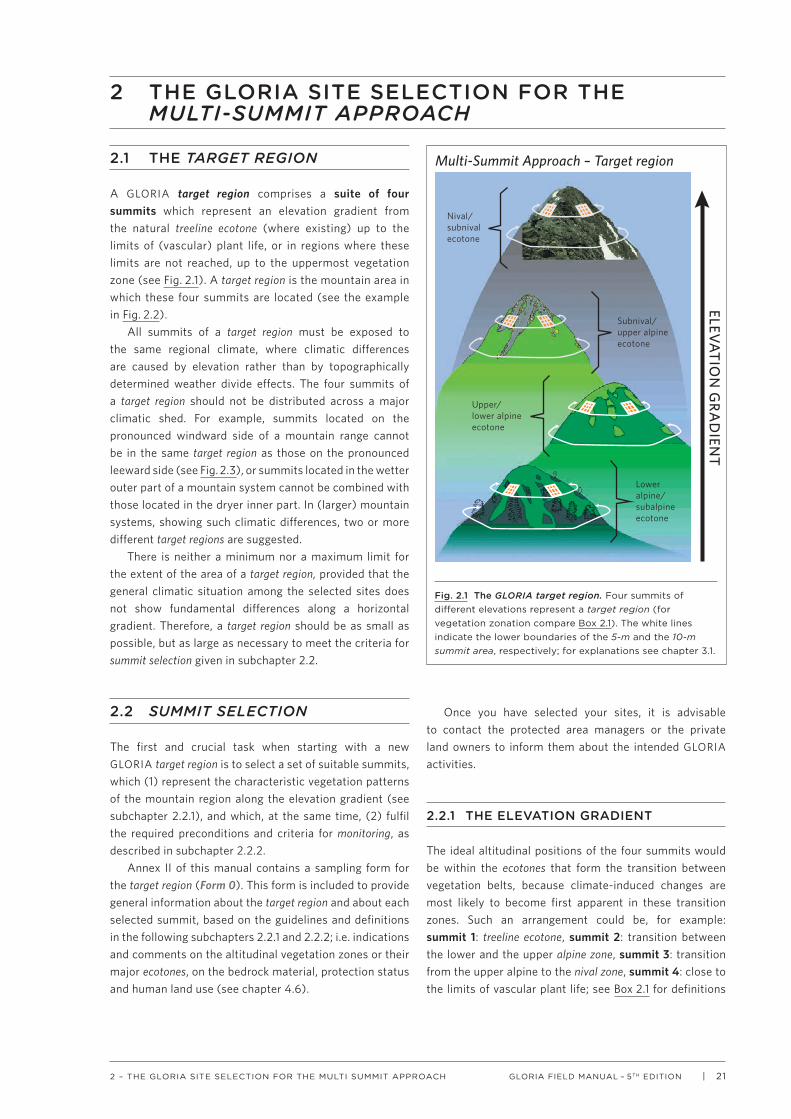
A GLORIA target region comprises a suite of four summits which represent an elevation gradient from the natural treeline ecotone (where existing) up to the limits of (vascular) plant life, or in regions where these limits are not reached, up to the uppermost vegetation zone (see Fig. 2.1). A target region is the mountain area in which these four summits are located (see the example in Fig. 2.2).

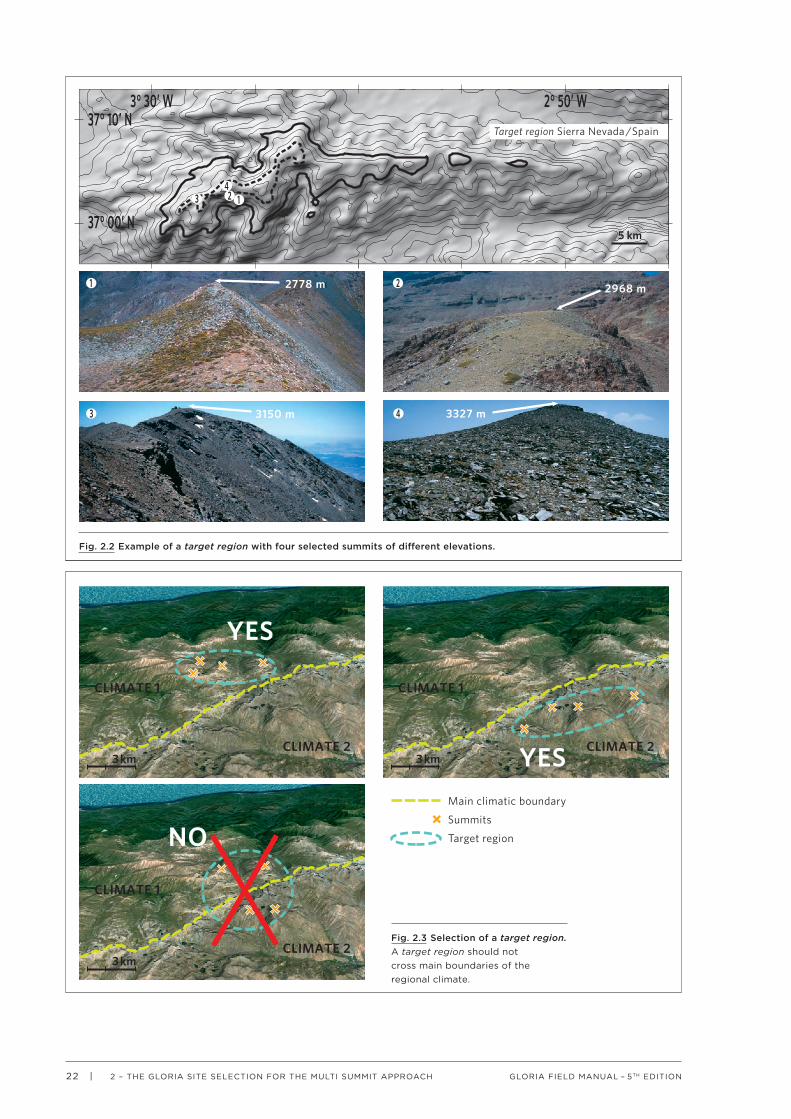
All summits of a target region must be exposed to the same regional climate, where climatic differences are caused by elevation rather than by topographically determined weather divide effects. The four summits of a target region should not be distributed across a major climatic shed. For example, summits located on the pronounced windward side of a mountain range cannot be in the same target region as those on the pronounced leeward side (see Fig. 2.3), or summits located in the wetter outer part of a mountain system cannot be combined with those located in the dryer inner part. In (larger) mountain systems, showing such climatic differences, two or more different target regions are suggested.

There is neither a minimum nor a maximum limit for the extent of the area of a target region, provided that the general climatic situation among the selected sites does not show fundamental differences along a horizontal gradient. Therefore, a target region should be as small as possible, but as large as necessary to meet the criteria for summit selection given in subchapter 2.2.

2.2 SUMMIT SELECTION

The first and crucial task when starting with a new GLORIA target region is to select a set of suitable summits, which (1) represent the characteristic vegetation patterns of the mountain region along the elevation gradient (see subchapter 2.2.1), and which, at the same time, (2) fulfil the required preconditions and criteria for monitoring, as described in subchapter 2.2.2.

Annex II of this manual contains a sampling form for the target region (Form 0). This form is included to provide general information about the target region and about each selected summit, based on the guidelines and definitions in the following subchapters 2.2.1 and 2.2.2; i.e. indications and comments on the altitudinal vegetation zones or their major ecotones, on the bedrock material, protection status and human land use (see chapter 4.6).

Once you have selected your sites, it is advisable to contact the protected area managers or the private land owners to inform them about the intended GLORIA activities.

2.2.1 THE ELEVATION GRADIENT

The ideal altitudinal positions of the four summits would be within the ecotones that form the transition between vegetation belts, because climate-induced changes are most likely to become first apparent in these transition zones. Such an arrangement could be, for example: summit 1: treeline ecotone, summit 2: transition between the lower and the upper alpine zone, summit 3: transition from the upper alpine to the nival zone, summit 4: close to the limits of vascular plant life; see Box 2.1 for definitions

2 THE GLORIA SITE SELECTION FOR THE MULTI-SUMMIT APPROACH

ELEVATION

GRA

DIEN

T

Multi-Summit Approach – Target region

Subnival/upper alpineecotone

Upper/lower alpineecotone

Lower alpine/subalpineecotone

Nival/subnivalecotone

Fig. 2.1 The GLORIA target region. Four summits of different elevations represent a target region (for vegetation zonation compare Box 2.1). The white lines indicate the lower boundaries of the 5-m and the 10-m summit area, respectively; for explanations see chapter 3.1.

22 | GLORIA FIELD MANUAL – 5TH  EDITION2 – THE GLORIA SITE SELECTION FOR THE MULTI SUMMIT APPROACH

Fig. 2.3 Selection of a target region. A target region should not cross main boundaries of the regional climate.

×Main climatic boundary

Summits

Target region

3 km

CLIMATE 1

CLIMATE 2

×× × ×

3 km

CLIMATE 1

CLIMATE 2×

× × ×

3 km

CLIMATE 1

CLIMATE 2

×

××

×NO

YES

YES

43 2 1

37° 00’ N

37° 10’ N2° 50’ W3° 30’ W

5 km

Target region Sierra Nevada /Spain

1 2

43

2778 m 2968 m

3150 m 3327 m

Fig. 2.2 Example of a target region with four selected summits of different elevations.

| 23GLORIA FIELD MANUAL – 5TH  EDITION2 – THE GLORIA SITE SELECTION FOR THE MULTI SUMMIT APPROACH

of vegetation belts. This ideal case, however, may be rather theoretical because obvious boundaries marking the limits of vegetation zones are often lacking. On the other hand, summit areas usually represent ecotonal situations anyway, e.g. along the gradient from the northern to the southern slope of the summit. Therefore, the summit selection may not lay stress on an exhaustive search for ecotones, but should focus on finding a series of summits which represent an elevation gradient of vegetation patterns, characteristic for the respective mountain region. The summit sites may be distributed in equal elevation intervals, as far as this is possible.

Mountain regions, where the alpine life zone does not show a clear vertical zonation should not be excluded. This is particularly the case, where mountains only slightly extend into the alpine life zone and where alpine biota are restricted to a narrow vertical belt. These biota are considered to be particularly prone to climate-induced

threats. In such cases, the selected summits are to be positioned in short vertical distances to each other.

Four summits are required for the basic arrangement within a target region. Exceptionally, a target region may consist of only three summits, e.g. where three suitable summits are available, but a fourth appropriate summit site is really absent. Three summits, however, is the minimum number to represent an elevation gradient, and thus three summits is the absolute minimum requirement to be considered as a GLORIA target region.

Until this point, any mountain region that extends into the alpine life zone is potentially appropriate for a GLORIA target region. In addition, however, GLORIA summits must meet several criteria (subchapter 2.2.2) which are crucial for applying standardised and practicable observation settings. Not all mountain areas may meet these criteria – and it is better to shift to another area rather than to establish a target region with inappropriate summit sites.

The GLORIA target regions are restricted to areas extending from the low-temperature determined treeline ecotone upwards; i.e. the area which coincides with the alpine life zone. Therefore, some definitions (compare Grabherr et al. 2003, Körner 2003, Nagy & Grabherr 2009, Grabherr et al. 2010, Körner et al. 2011, Körner 2012) and considerations are given here.u The forestline (or timberline), marking the lower limit of the treeline ecotone, is defined as the line where closed (montane) forests end. u The treeline is the line where groups of trees taller than 3 m end.u The tree species line is the line beyond which no adult individuals of tree species, including prostrate ones or scrub, occur.u The treeline ecotone is the zone between the forest line and the tree species line. u The alpine life zone is the area from the forestline upwards and, thus, includes the treeline ecotone, the alpine zone, the alpine-nival ecotone, and the nival zone.u The alpine zone (or alpine belt) is the zone between the treeline and the upper limit of closed vegetation (cover >20–40%, but can be less in arid regions), where vegetation is a significant part of the landscape and its physiognomy. The alpine zone of some mountain regions is

further subdivided into a lower alpine zone (the zone where dwarf-shrub communities are a major part of the vegetation mosaic) and an upper alpine zone (where grassland, steppe-like and meadow communities are dominating). For regional variants, different terms are widely used, such as cryoro-mediterranean ( Fernández Calzado & Molero Mesa 2011), afro-alpine, high-andean, páramo, puna (Cuesta et al. 2012, Sklenář et al. 2013), which are subsumed here as alpine zone.u The nival zone is the zone of ice, permanent snow, and/or bare bedrock material being mostly uninhabitable by vascular plants. Cryptogam species such as lichens and bryophytes may occur besides few outposts of scattered individual vascular plants or scant patchy vegetation at thermally favourable microsites. Vegetation is not a significant part of the landscape.u The alpine-nival ecotone (or subnival zone) is the transition between the upper alpine and the nival zone. The position of this ecotone can be highly related to the duration of summer-snowpack (cf. Gottfried et al. 2011) and might coincide with the permafrost limit in many mountain regions.

Considerations concerning the treeline ecotone: For an opti-

mal applicability of the sampling methods, the vegetation on the lowest summit of a target region should not be dominated by tree species or tall shrubs, because the method is particularly designed for low-stature dwarf-growing alpine vegetation. Thus, for the lowest summit, a site within the upper part of the treeline ecotone should be selected, where trees or shrubs occur only sparsely. Further, the summit should lie within the potential natural treeline ecotone, and not at the present treeline, if the latter has been lowered significantly owing to human interference.

In mountain systems where no treeline exists because of aridity, or where the treeline is substituted by human land use with pastures, the alpine life zone may be defined as that part of the landscape, which was shaped by glaciers (which were present at least in the Pleistocene) and where frost is an important factor for pedogenesis and substrate structure (compare Troll 1966). Finally, the occurrence of ruggedness in the landscape is a crucial determinant of high mountain environments and would exclude flat altiplanos, such as found in parts of the southern central Andes or in the Qinghai-Tibetan plateau (Körner et al. 2011).

BOX 2.1 VEGETATION ZONATION IN HIGH MOUNTAIN AREAS

24 | GLORIA FIELD MANUAL – 5TH  EDITION2 – THE GLORIA SITE SELECTION FOR THE MULTI SUMMIT APPROACH

2.2.2 CONSIDERATIONS AND CRITERIA FOR THE SUMMIT SELECTION

GLORIA summit sites not only comprise the uppermost peak of a mountain, but the summit area down to the 10-m contour line below a mountain’s highest point. Such summit sites may be located around the very top of a mountain system or on a less prominent summit of the mountain system, the latter being often of lesser attractivity for mountain tourism. Even any hump in a ridge which protrudes more than about 20 elevation metres above the surrounding land features may serve as a suitable summit site.

Given the vast geomorphological and ecological variation in alpine mountain top environments, the following six ‘criteria’ (A-F) are recommendations, rather than strict criteria. Nevertheless, they are important to be taken into account when selecting summit sites for the long-term surveillance of high-mountain biota.

These criteria are not ranked for their priority but along a sequence starting with those that can be evaluated already in the initial planning phase, just by using maps, aerial and satellite images and literature, to those where a visit of a candidate summit site is required. For the final decision, an on-site inspection of each summit is necessary in any case.

 A  VO LC A N I S M  GLORIA sites should lie outside of areas where active volcanism is an obvious factor shaping the prevalent vegetation patterns and species composition. Impacts arising from volcanic processes such as eruptions, ash rain as well as thermal influences of habitat conditions would strongly mask any climate change-related signal and a high frequency of eruption raises the risk of complete loss of permanent plots. Dormant volcanoes may be considered as suitable, if eruption activity dates back long enough to be of negligible influence for the current vegetation patterns.

››  Avoid areas with active or dormant volcanism that still influences the prevailing vegetation.

B CONSISTENT LOCAL CLIMATE Ideally, all four summit sites of a target region should be exposed to the same local climate, where the only climatic differences are caused by their different altitudinal positions. It is, however, not trivial to distinguish between climate influences just caused by elevation from those caused by a particular topography and, thus, decisions would be difficult. The main point, however, that can be more easily considered is to avoid that the set of four summits is distributed across a pronounced climatic divide. For example, a target region’s set of four sites should not include sites in a pronounced windward side as well as sites in dryer and warmer leeward or interior parts of mountain ranges (Fig.  2.3). Instead, each climatically clearly distinguishable part of a mountain system should be treated as different target regions.

››  Avoid that summit sites within a target region are distributed across pronounced climatic divides.

 C BEDROCK OF THE SUMMIT AREA All summits within a target region should be composed of similar bedrock. In particular, the mingling of summits of strongly contrasting bedrock, e.g. calcareous and siliceous, within one target region should be avoided, because differences in species richness and species composition would be confounded by substratum-related factors. In regions with nearby occurrences of such different bedrock types, establishing of two ‘target regions’ separating the contrasting substrates of the same region, is a valuable solution for comparing different habitats (such as in the Swiss National Park region or in the White Mountains, California).

››  Avoid that summit sites within a target region have contrasting bedrock types.

 D HUMAN DISTURBANCE PRESSURE In the ideal case, GLORIA summits lie in pristine or near-natural environments that are not obviously altered through direct human interference. Areas should not be affected by heavy pressure from human land use (see Fig.  2.4) as impacts by grazing animals (trampling, grazing, and fertilising) and trampling effects by hikers may cause substantial changes in species composition and vegetation patterns. Such effects are likely to mask climate-induced changes.

GRAZING AREA

1

23

4

1-4 | APPROPRIATE GLORIA-SUMMITSTOURIST SUMMIT

TOURIST SUMMIT

Fig. 2.4 Avoid direct human impact. Summits frequently visited by tourists or located in an area of heavy grazing (either by livestock or by anthropogenically strongly raised numbers of wild ungulates) are not appropriate.

| 25GLORIA FIELD MANUAL – 5TH  EDITION2 – THE GLORIA SITE SELECTION FOR THE MULTI SUMMIT APPROACH

In a number of mountain ranges, we still find rather pristine tree lines and alpine zones, such as in parts of North America and other boreal to arctic regions or in New Zealand and parts of the southern Andes. In many of the European mountain areas, in large parts of the Andes and mountains of Asia and Africa, however, traditional land use – mainly mountain pastoral and/or burning practices – have altered the treeline ecotone and, to a minor extent, also the lower alpine zones (e.g. Bock et al. 1995, Molinillo & Monasterio 1997, Adler 1999, Bridle & Kirkpatrick 1999, Spehn et al. 2006, Yager et al. 2008a, Halloy et al. 2010). In such cases, the selection should focus on the least affected sites, preferably in national parks or nature reserves, where human disturbance pressure can be expected to remain low in the future (see also Box  4.6). Fortunately, globally around 35% of the little impacted mountain regions are covered by nationally designated protected areas (Rodríguez-Rodríguez & Bomhard 2012, Pauli et al. 2013). A moderate traditional pastoralism, however, is less critical if land use practices remained quite the same over centuries concerning both type and intensity. Such sites may be suitable as GLORIA sites. Heavily overgrazed areas, where plant communities have obviously changed (grazing indicator plants), however, should not be used as GLORIA sites. Further, those areas where type and intensity of human land use changed strongly during recent decades or during the past century should be avoided as far as possible. Such pronounced changes in traditional land use patterns, either through abandonment of mountain farming or its intensification, are likely to cause overlaps with an overall footprint of climate warming.

››  Avoid heavily overgrazed sites, tourist summits and areas with strong recent changes in land use practices.

 E GEOMORPHOLOGIC SHAPE OF THE SUMMIT AREA Summits should be of “moderate” geomorphologic shape (for a definition see the glossary under: moderately shaped summit). Very steep summits as well as flat tops, forming plateaus, are unsuitable for the application of the Multi-Summit Approach (Fig.  2.5). Steep mountain peaks and summits with very unstable substrate should be avoided, first, because of safety reasons. In the usual situation at GLORIA surveys, where several persons work at the same time, great care because of rock falls is necessary. Steep and unstable sites, therefore, must be excluded because of the enhanced accident risk. Second, many steep summits have only few micro-habitats for plants to establish, because of the dominance of rocky habitats, and are thus of little use for observing vegetation changes. Third, steep sites would require the use of climbing equipment and, therefore, would prolong the required time. Flat summit areas are disadvantageous as the four main aspect situations are absent, and the sampling area becomes larger, the flatter the terrain is. Flat and plateau-like mountain tops, however, are typical for several mountain regions on all continents, where “moderately shaped” summits may be difficult to find. In such cases, some modifications of the method, described in Box 3.4, may be considered.

This topography criterion absolutely requires an inspection in the field. Check the steepness of the summit terrain and if distances from the highest summit point towards the four cardinal directions are reasonable within the uppermost 5 and 10 metres in altitude (less than 50 m and 100 m in distance, respectively, but see Box 3.4).

››  Avoid steep and unstable summits, use flat sites only in absence of alternatives.

5m10m

5m10m

5m10m moderate

flat/plateau

5m10m

D moderate

moderate

5m

10m

steepa c d

b

e

Fig. 2.5 Geomorphologic shape. a Summit areas which are too steep (either for recording or for providing habitats for vascular plants) are to be avoided.

b Flat, plateau-shaped summits are not appropriate: the

recording area would be too large; but an option to include even such flat summits (when no moderately shaped summits are present) is given in Box 3.4

c - e Moderately shaped summits should be selected.

26 | GLORIA FIELD MANUAL – 5TH  EDITION2 – THE GLORIA SITE SELECTION FOR THE MULTI SUMMIT APPROACH

 F HABITAT CONTEXT The prevalent vegetation on a GLORIA summit should be representative for the typical species occurring in the respective elevation belt. The patterns of microhabitats populated by vascular plants or, at the high summits, of potential sites where plants could establish, should be similar to the average situation at the given elevation. Summits dominated by solid rock (irrespective of steepness), by unstable scree fields or by large boulder fields, should be avoided.

››  Avoid summits where habitats or potential habitats for vascular plants are scarce.

| 27GLORIA FIELD MANUAL – 5TH  EDITION3 – STANDARD SAMPLING DESIGN OF THE MULTI SUMMIT APPROACH

This chapter contains the detailed description of the basic plot design for the Multi-Summit Approach and how to establish a monitoring site on a mountain summit. The setup procedure is described in detail along  WORK STEPS   A - G .

CONTENT OVERVIEW WITH THE STANDARD  WORK STEPS   A - G 

3.1 Plot types and design outline  283.2 Materials and preparations  303.3 Setup of the permanent plots  303.3.1 The highest summit point (HSP): determination of the principal reference point  30  WORK STEP   A  Marking the HSP  303.3.2 Establishing the 1-m² quadrats in 3 m × 3 m quadrat clusters and the summit area corner points  31  WORK STEP   B  Determination of the principal measurement lines  32  WORK STEP   C  Fixing the 3 m × 3 m quadrat clusters  33  WORK STEP   D  Measuring the distances and the magnetic compass directions from the HSP to the quadrat cluster corner points  343.3.3 Establishing the boundary lines of the summit areas and the summit area sections  34  WORK STEP   E  Establishing the boundary line of the 5-m summit area  36  WORK STEP   F Establishing the boundary line of the 10-m summit area  36  WORK STEP   G  Dividing the summit areas into sections by establishing intersection lines  36

3 STANDARD SAMPLING DESIGN OF THE MULTI-SUMMIT APPROACH

28 | GLORIA FIELD MANUAL – 5TH  EDITION3 – STANDARD SAMPLING DESIGN OF THE MULTI SUMMIT APPROACH

3.1 PLOT TYPES AND DESIGN OUTLINE

The sampling design for each summit consists of:u Sixteen 1-m² quadrats (Fig. 3.1), arranged as the four corner quadrats of the four 3 m × 3 m quadrat clusters in all four main compass directions, yielding

16 1-m² quadrats per summit (=16-quadrat area).u Summit area sections (Fig.  3.1), with four sections in the upper summit area (5-m summit area) and four sections in the lower summit area (10-m summit area). The size of the summit area section is not fixed but depends on the slope structure and steepness.

N

HSP

1m2m

3m4m

5m6m

7m8m

9m

10m

HSP (highest summitpoint)

Contour line(metres belowthe highest summitpoint)

Principalmeasurement line

Measurement linefor quadrat clustercorners

3m × 3m quadrat clusterwith four permanent quadrats (filled)

Boundary of summit areas

Upper summit area= 5-m summit area

Lower summit area= 10-m summit area

Intersection linedividing the summit area intosections

1m2m

3m4m

5m6m

7m8m

9m10m

Quadrat cluster

Summit area sections Temperature measurement

Highest summit point (HSP)

S SEE

a

b

Fig. 3.1 The Multi-Summit sampling design shown on an example summit. a  Oblique view with schematic contour lines; b Top view. The 3 m × 3 m quadrat clusters and the corner points of the summit areas are arranged in the main geographical

directions. Each quadrat cluster can be arranged either on the left or on the right side of the principal measurement line, depending on the local terrain and habitat situation (this is independent of the respective settings of the other three quadrat clusters). As a general rule, left and right is always defined facing to the highest summit point.

| 29GLORIA FIELD MANUAL – 5TH  EDITION3 – STANDARD SAMPLING DESIGN OF THE MULTI SUMMIT APPROACH

An illustration of the plot arrangements is shown in Fig. 3.1 with an oblique and a top view on an example summit. Fig.  3.2 shows the scheme of the sampling design with the code numbers of all measurement points and sampling plots.

The full setup and the standard recording procedure requires between two and about six days per summit for

a team of four investigators (dependent on vegetation density, species richness and site accessibility). This time estimate includes the sampling of vascular plants, but excludes the recording of bryophytes and lichens on the species level.

Note that at least two fieldworkers are absolutely necessary for establishing the permanent recording

The corner points:

Upper summit area= 5-m summit area

Lower summit area= 10-m summit area

Intersection lines:divide the summit areas into eight summit area sections (e.g. N-5m-SA, N-10m-SA)

Position of the corner points

HSP (Highest summit point)

Principal measurement lines

Measurement lines from the HSP to 3 corner points of each quadrat cluster

Boundary of summit areas(which does not follow the contour line)

p10m-N, p10m-E, p10m-S, p10m-W: the 4 corner points at the 10-m level; they determine the lowerlimit of the 10-m summit area

The principal measurement line for each main direction starts at the HSP,runs through one of the points at the 5-m level (e.g. p5m-N11 or p5m-N31)and ends at the corner points at the 10-m level

pNE-5, pNE-10, pSE-5, pSE-10, pSW-5, pSW-10, pNW-5, pNW-10 :the 8 corner points at the intersection lines (these points usually lie above the 5-m level and the 10-m level, respectively)

The summit area sections are delimited by these points,by the HSP, and the points p5m-... and p10m...

N11

N13N33

N313m x 3m quadrat cluster:four quadrat clusters, each with four 1m x 1m quadrats =16 1m2 sampling units(forming together the 16-quadrat area)

p5m-N11, p5m-E31, p5m-E11, p5m-S31, p5m-S11, p5m-W31, p5m-W11, p5m-N31:the 8 lower corner points of the 3m x 3m quadrat clusters at the 5-m level

They determine the position of the quadrat clusters and the lower limit of the 5-m summit area

p-N13, p-E13, p-S13, p-W13, p-N33, p-E33, p-S33, p-W33 :the 8 upper corner points of the quadrat clusters

10-m contour line

5-m contour line

N-5m-SA

N-10m-SA

S-10m-SA

S-5m-SA

W-1

0m

-SA E-10

m-SAW

-5m

-SA E-5m

-SA

HSPp5m-W11

p5m-W31

p-W13

p-W33

p5m-N11p5m-N31

p-N13p-N33

p5m-E11

p5m-E31

p-E13

p-E33

p5m-S11p5m-S31

p-S13p-S33

p10m-E

p10m-N

p10m-W

p10m-S

pNW-10

pNW-5

pNE-10

pNE-5

pSE-10

pSE-5

pSW-10

pSW-5

N11

N13N33

N31

S11

S13S33

S31

E11E13

E33 E31

W11 W13

W33W31

N10 m

Fig. 3.2 Scheme of the Multi-Summit sampling design. The standard sampling design comprises 16 1-m² quadrats and eight summit area sections (SASs). Note that only the corner points in the cardinal directions (N, E, S, W) lie at the 5-m respectively 10-m contour line below the highest summit point, whereas the corner points at the intermediate directions (NE, SE, SW, NW) usually lie above the 5-m respectively the 10-m level. The latter points are determined only as the crossing points of summit area boundary lines (i.e. straight lines connecting the corner points in the cardinal directions) and the intersection lines.

30 | GLORIA FIELD MANUAL – 5TH  EDITION3 – STANDARD SAMPLING DESIGN OF THE MULTI SUMMIT APPROACH

areas and settings, but a team of at least four persons is highly recommended. However, be aware of increased disturbance when you have a large team.

3.2 MATERIALS AND PREPARATIONS

The following materials and tools are needed for site setup and recording (for your fieldwork preparation see the checklist in Annex I of the field manual):

u For measuring the position of plots and corner points of the summit area: two rolls of flexible 50-m measuring tape (the use of shorter tapes is not recommendable); a compass (recommended: Suunto KB-14/360); a clinometer (recommended: Suunto PM-5/360PC); two small rolls of measuring tapes (e.g. of 3 m length). An altimeter and a GPS may be useful supplementary devices.u For delimiting the 1-m² quadrats: four sampling grids of 3 m × 3 m with 1 m × 1 m cells. These grids should be made of flexible measuring tapes fitted together to a grid with small metal blanks or with a strong adhesive tape (for instructions see Fig. AI.1 in Annex I). About 100 pieces of ordinary 100 mm nails and thin wire for mounting the sampling grids in the field, adhesive tape to repair the grids in the field.u For delimiting the summit area: two rolls of thin string (each about 500 m long) and four rolls of the same type (about 100 m each); check if strings are on an easy-to-handle spool. The length of these strings depends on the summit shape (the flatter the summit, the longer the string must be). The colour of the string should contrast with the surface colour (e.g. bright yellow is a good choice).u For permanent marking: per summit about 80 aluminium tubes (0.8 or 1  cm in diameter) in various lengths (between 10 and 25  cm) or other material appropriate for the relevant substrate (e.g. durable white or yellow paint) and a small chisel (for marking the highest summit point).u For photo documentation (see chapter 4.4): a digital camera for high-resolution photos, wide-angle and standard lenses or a zoom wide-angle to standard lens (wide-angle for depicting a 1-m² area from a top-view position); a small blackboard (e.g. 15 × 20 cm) plus chalk for writing the plot number and date; a signal stick or rod (1.5 to 2 m) to mark the corner points on the photos.u For the recording procedures (see chapters 3 and 4): sampling sheets in a sufficient number of copies: the Forms 0, 1, 2, 3, 4 in Annex II and downloadable from the GLORIA website under

‘Methods’); compass, clinometer or electronic spirit level (i.e. the same devices as used for plot positioning); transparent templates for cover estimations (see Fig.  AI.3a & b in Annex I); one wooden (or aluminium) grid frame of 1 m × 1 m inner width and 100 crosshair points distributed regularly over the plot (see Fig. 4.2 and Fig. AI.2 in Annex I); a sampling pin of 2 mm diameter for point recording (e.g. a knitting needle of 2 mm diameter).u For permanent temperature measurements (see chapter 4.3): miniature temperature data loggers (four per summit, i.e. 16 per target region), logger protocol sheet (Form 4), watch, gardening trowel, for data readout: laptop, dongle.u For supplementary methods (see chapter 5) Use a wooden (or aluminium) frequency grid-frame of 1 m × 1 m inner width (Fig.  5.1) for subplot-frequency counts, which has a different arrangement of strings than the pointing frame, and the sampling sheet Forms 5-S in Annex II.

For the supplementary 10 m × 10 m squares you need additional flexible measuring tapes: one roll of 50 m (for delimitation) and one of at least 10 m (for line-pointing) and the sampling sheet Form 6-S in Annex II.

3.3 SETUP OF THE PERMANENT PLOTS

Setup and measurements of plot positions such as distances and compass bearings from the highest summit point (HSP) to the plot corners must be made carefully and all entries into the measurement sheet (Form 1) should be double-checked. The data entered into Form 1 are crucial for the automated calculation of the area size of the summit area sections (SAS) and the processing of outline drawings.

3.3.1 THE HIGHEST SUMMIT POINT (HSP): DETERMINATION OF THE PRINCIPAL REFERENCE POINT

The highest summit point (HSP) is the starting point of all measurements. The HSP is usually the middle of the summit area of moderately shaped summits. Rocky outcrops at one side of the summit area, which may exceed the elevation of the middle culmination point (compare Fig. 2.5d), should be ignored.

 WORK STEP   A   Marking the HSP

This point should be marked with a small cross cut into the

solid rock by using a chisel (Fig. 3.3). For sites lacking a

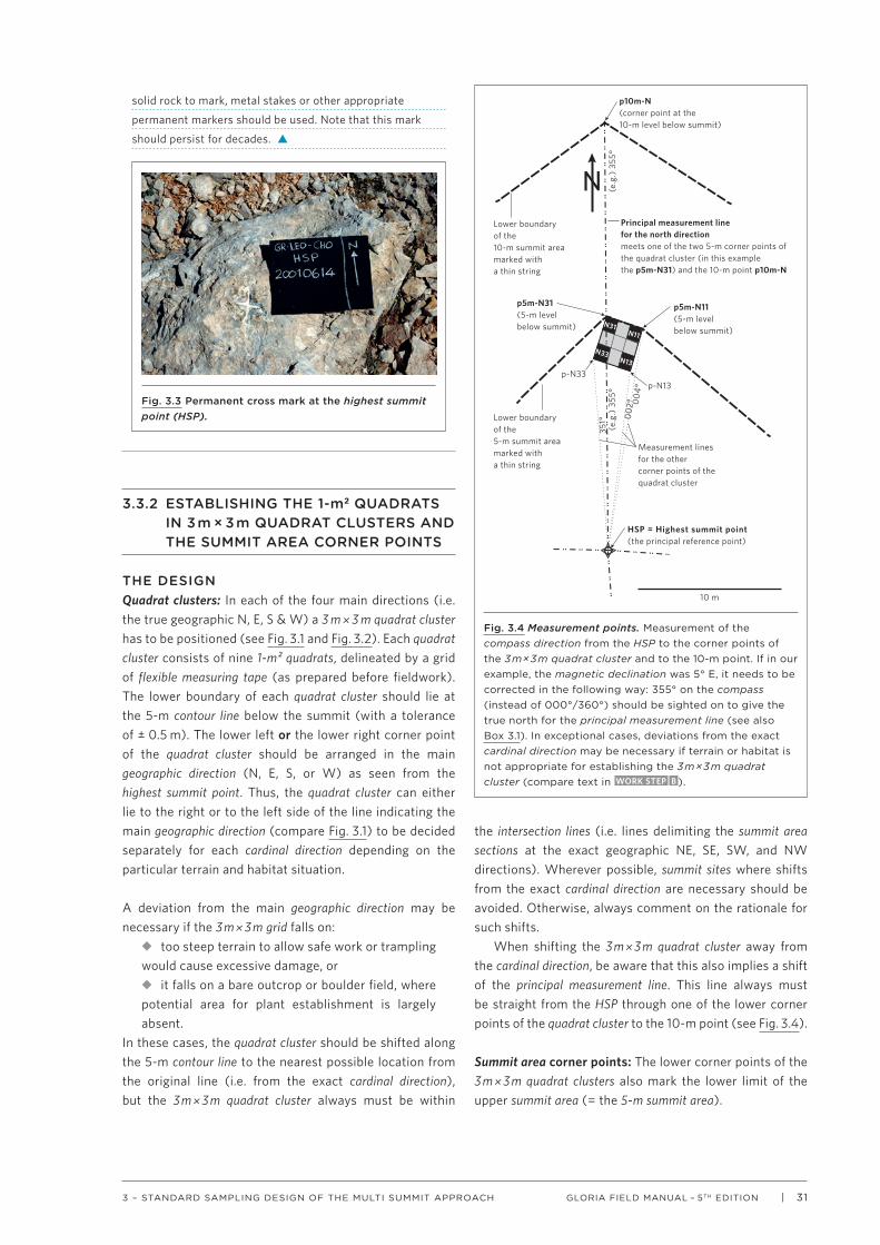
| 31GLORIA FIELD MANUAL – 5TH  EDITION3 – STANDARD SAMPLING DESIGN OF THE MULTI SUMMIT APPROACH

solid rock to mark, metal stakes or other appropriate

permanent markers should be used. Note that this mark

should persist for decades. s

3.3.2 ESTABLISHING THE 1-m2 QUADRATS IN 3 m × 3 m QUADRAT CLUSTERS AND THE SUMMIT AREA CORNER POINTS

THE DESIGNQuadrat clusters: In each of the four main directions (i.e. the true geographic N, E, S & W) a 3 m × 3  m quadrat cluster has to be positioned (see Fig. 3.1 and Fig. 3.2). Each quadrat cluster consists of nine 1-m² quadrats, delineated by a grid of flexible measuring tape (as prepared before fieldwork). The lower boundary of each quadrat cluster should lie at the 5-m contour line below the summit (with a tolerance of ± 0.5  m). The lower left or the lower right corner point of the quadrat cluster should be arranged in the main geographic direction (N, E, S, or W) as seen from the highest summit point. Thus, the quadrat cluster can either lie to the right or to the left side of the line indicating the main geographic direction (compare Fig. 3.1) to be decided separately for each cardinal direction depending on the particular terrain and habitat situation.

A deviation from the main geographic direction may be necessary if the 3 m × 3 m grid falls on:

u too steep terrain to allow safe work or trampling would cause excessive damage, oru it falls on a bare outcrop or boulder field, where potential area for plant establishment is largely absent.

In these cases, the quadrat cluster should be shifted along the 5-m contour line to the nearest possible location from the original line (i.e. from the exact cardinal direction), but the 3 m × 3 m quadrat cluster always must be within

the intersection lines (i.e. lines delimiting the summit area sections at the exact geographic NE, SE, SW, and NW directions). Wherever possible, summit sites where shifts from the exact cardinal direction are necessary should be avoided. Otherwise, always comment on the rationale for such shifts.

When shifting the 3 m × 3 m quadrat cluster away from the cardinal direction, be aware that this also implies a shift of the principal measurement line. This line always must be straight from the HSP through one of the lower corner points of the quadrat cluster to the 10-m point (see Fig. 3.4).

Summit area corner points: The lower corner points of the 3 m × 3 m quadrat clusters also mark the lower limit of the upper summit area (= the 5-m summit area).

Fig. 3.3 Permanent cross mark at the highest summit point (HSP).

Fig. 3.4 Measurement points. Measurement of the compass direction from the HSP to the corner points of the 3 m × 3 m quadrat cluster and to the 10-m point. If in our example, the magnetic declination was 5° E, it needs to be corrected in the following way: 355° on the compass (instead of 000°/360°) should be sighted on to give the true north for the principal measurement line (see also Box 3.1). In exceptional cases, deviations from the exact cardinal direction may be necessary if terrain or habitat is not appropriate for establishing the 3 m × 3 m quadrat cluster (compare text in  WORK STEP   B ).

10 m

p5m-N11(5-m levelbelow summit)

p5m-N31(5-m levelbelow summit)

p-N33p-N13

p10m-N (corner point at the 10-m level below summit)

Principal measurement linefor the north directionmeets one of the two 5-m corner points of the quadrat cluster (in this example the p5m-N31) and the 10-m point p10m-N

(e.g

.) 3

55°

004°

351° 00

2°

(e.g

.) 3

55°

Measurement linesfor the other corner points of the quadrat cluster

HSP = Highest summit point(the principal reference point)

Lower boundaryof the10-m summit areamarked with a thin string

Lower boundaryof the5-m summit areamarked with a thin string

N31N11

N33N13

N

32 | GLORIA FIELD MANUAL – 5TH  EDITION3 – STANDARD SAMPLING DESIGN OF THE MULTI SUMMIT APPROACH

The four lower corner points of the lower summit area (= the 10-m summit area) lie along the straight line connecting the HSP and the 5-m corner point (= the principal measurement line), at 10 m elevation below the HSP (compare Fig. 3.1 and Fig. 3.2).

The suggested working sequence described in this subchapter must be repeated for each main geographical direction (N, E, S, & W) and is demonstrated here for the N-direction with the following  WORK STEPS   B  -  D  (compare with Fig. 3.2, Fig. 3.4 and Fig. 3.5; see also the measurement protocol sheet (Form 1).

 WORK STEP   B   Determination of the principal

measurement lines (the compass direction, the vertical

extension, and the length)

i.e. from the HSP straight down through a point at the 5-m

level to the endpoint at the 10-m level.

u Person A measures the eye-height of person B (i.e.

the distance from the sole of the boots to the eyes).

u Person A stands with a compass and the measurement

protocol (Form 1) at the HSP and fixes a 50-m measuring

tape at this point. He/she points out the geographic

N-direction (see Fig. 3.4, Fig. 3.5 and Box 3.1).

u Person B begins walking in the indicated geographic

N-direction unwinding the measuring tape and

focusing on the highest summit point with a clinometer.

When reaching an exact horizontal view of the HSP, a

temporary marker is placed on the ground. The elevation

difference between the marker and the HSP equals the

eye-height (i.e. the body length from feet to eyes) of

person B. This process is repeated until the 5-m point is

reached (see Fig. 3.5).

u When reaching the 5-m level, person B (or both)

decides if the location is appropriate for spreading

the 3 m × 3 m grid. If not, another location at the 5-m

level, positioned as close as possible to the exact

geographical N-direction, should be chosen. Whenever

such a deviation is necessary, always stay within the

area delimited by the NW and the NE intersections lines

which will be established later in  WORK STEP   G ).

u The determined point at the 5-m level (this will be

either point p5m-N11 or p5m-N31, see  WORK STEP   C ), will

The magnetic N-direction can deviate considerably from the geographic N-direction in some regions and can change in comparatively short periods of time. Therefore, the magnetic declination (i.e. the angle between the direction of the geographic North Pole and the magnetic North Pole) has to be identified and indicated on the measurement protocol sheet (Form 1). Check the region’s magnetic declination before starting fieldwork.

The current magnetic declination of any place on the globe can be obtained, for example, from the web site of the US-National Geophysical Data Center, Boulder: www.ngdc.noaa.gov/geomag-web/ #declination

To fix, for example, a point in the geographic N-direction the measuring person defines:

u the magnetic N-direction with the compass, u corrects it for the magnetic declination and u guides the person, who fixes the points, to the corrected geographic N-direction.

This applies to all directions (N, E, S, W as well as to NE, SE, SW, NW; see also below in this box).

Magnetic declination: The magnetic declination should be indicated in degrees (360° scale) with its correct sign (+ or – ) at the top of the measurement protocol (Form 1).

For example, – 6 ( = 6° W = 6° west of the geogr. North Pole), +20 (= 20° E = 20° east of the geogr. North Pole). In southern Europe and in the European Alps, the magnetic declination is currently only between – 1° and +4°. There are larger declinations, e.g. in N-Sweden or in the Central Caucasus (currently between +6 and +7°), Southern Ural (about +12°), Northern Ural (+24°), Tierra del Fuego, Argentina (+13°), Central Brooks Range, Alaska (about +20°) or on central Ellesmere Island, N-Canada (about – 54°). These ex-amples show that it is important to consider the magnetic declination for establishing the permanent plots, when using a field compass.

The magnetic declination must be considered for the determination of all four principal measurement lines as well as for the four intersection lines. For example, the corrected

compass bearings at a given magnetic declination of +5 (5° E) are 355° for true/geographic N, 085° for E, 175° for S, 130° for SE; the corresponding values at a magnetic declination of –10 (10° W) are: 010° (for true N), 100° (E), 190° (S), 145° (SE). That means, e.g. for the N-direction and a magnetic declination of +5: use the compass bearing 355° to fix the principal measurement line and the N-cluster (see Fig. 3.4).

Please note: In any case, only the measured magnetic compass bearing has to be entered into the protocol sheet (Form 1), i.e. degrees on the 0-360° scale as indicated on the compass (see also Fig. 3.4). This is relevant for all numeric indica-tions of directions in the sampling protocols. For example, at a magnetic declination of +8 (8° E) write into your protocol sheet: 352° for the proper compass bearing of the true north direction, 37° for the true NE direction, 82° for the true east direction, and so forth.

For measuring compass directions, an accuracy of ± 2° can be normally reached with an ordinary field compass or ± 1° with a Suunto KB-14/360 compass.

BOX 3.1 COMPASS MEASUREMENTS

| 33GLORIA FIELD MANUAL – 5TH  EDITION3 – STANDARD SAMPLING DESIGN OF THE MULTI SUMMIT APPROACH

be marked with a small aluminium tube and with some

stones to aid the further setup procedure (in  WORK

STEP   C ).

u From the point at the 5-m level, person B continues

downward to the 10-m level, being guided by person A.

Note that the HSP and the finally determined position

of the points at the 5-m and the 10-m levels (e.g. HSP,

p5m-N11 and p10m-N) must lie on the same straight line.

The 10-m point (p10m-N) will be marked again with a

small aluminium tube and some stones.

u Person B tightens the 50-m measuring tape (held by

person A to ensure that the tape is straight through the

marked 5-m point), and calls the distance read from the

measuring tape at the 10-m point (see Box 3.3).

u Person A enters the distance value into the protocol

(Form 1).

u Person A (standing on the HSP) focuses the compass

on person B (standing on the 10-m point) and reads

the magnetic compass direction. If person B is not

visible to person A, person B holds up a signal rod

perpendicularly.

u Person A enters the (magnetic) compass bearing into

the protocol sheet (compare Box 3.1). s

 WORK STEP   C   Fixing the 3 m × 3 m quadrat clusters

After the principal measurement line with the positions at the

5-m and at the 10-m levels is determined, the 3 m × 3 m quadrat

cluster can be placed at the 5-m level (Fig. 3.2). This should

be done by two persons. Particular care is required at this step

to avoid trampling impacts in the plot area (see also Box 3.2).

u As shown in Fig. 3.1, the measured 5-m point is

either the left lower (e.g. p5m-N11) or the right lower

corner (e.g. p5m-N31) of the 3 m × 3 m grid. In the case

of p5m-N11, the grid is placed on the right side of the

principal measurement line, in the case of p5m-N31, on

the left side (in view to the HSP). The decision depends

on suitability of the local terrain and habitat situation.

Both points (p5m-N11 and p5m-N31) have to be on the

5-m level such that the left and right boundaries of the

quadrat cluster are more or less parallel to the slope.

u The corner points of each 1-m² quadrat of the grid

should be fixed at the surface as far as possible (some

corners may stay above the surface in a rugged terrain).

This can be done with ordinary 100 mm nails put

through the hole of the blanks (eyelets at the crossing

points of the 3 m × 3 m grid) or through the outer tape

material, and/or with stones or a thin wire.

u In addition, short aluminium tubes should be

5m5.

25m

0.25mdetermined by asmall measuringtape

10-m point

1 2

3 4

1.75m

1.75m

1.75m

5.25

m

Person A with compass (and the protocol sheet) stays on the HSP

Person B steps downwards with a clinometer and with a 50-m measuring tape which is fixed at the HSPHSP

5-m pointPerson B witha clinometer and asmall measuring tape

5.25

m

0.25mdetermined by asmall measuringtape

HSP

5m 5-m point

1.75m

1.75m

5.25

m1.7

5m

HSP HSP

5-m point

Fig. 3.5 Measurement of the vertical distances. Person A signals the compass direction (see Box 3.1), person B (with an eye-height of 1.75 m in this example), measures the vertical distance. 1 Three eye-heights down to the 5.25 m level (= 3× 1.75 m; i.e. it is depending on the actual eye-height of person B); 2 Measuring the remaining vertical distance (upwards in this example) and fixing of the 5-m point; 3 Three eye-heights down to the 10.25 m level; 4 Measuring the remaining vertical distance and fixing of the 10-m point (for measurement tolerances see Box 3.3).

BOX 3.2 TRAMPLING IMPACTS BY THE INVESTIGATORS

Trampling impacts during the setup and removal of plot grids as well as during the sampling should be minimised.

Strictly avoid stepping into the permanent 1-m² quadrats. Particular care must be taken, e.g. in some lichen- or bryophyte-dominated communities, snowbed and tall meadow vegetation or in unstable scree fields.

Sleeping pads, such as those commonly used by campers, may be useful during sampling, where terrain is appropriate.

1 2

3 4

34 | GLORIA FIELD MANUAL – 5TH  EDITION3 – STANDARD SAMPLING DESIGN OF THE MULTI SUMMIT APPROACH

positioned at the corners of the quadrats as permanent

marks, where applicable. Only the upper 1-2 cm of these

tubes should protrude above the surface in order to

avoid easy detection by hikers and mountaineers. Where

aluminium markers cannot be mounted (e.g. in shallow

soil or on solid rock), a small white or yellow point can

be painted with durable paint. Permanent marking with

durable material is essential in taller-growing vegetation

such as in alpine meadows, or in páramo and puna

vegetation, if solid rock is absent. s

 WORK STEP   D   Measuring the distances and the

magnetic compass directions from the HSP to the quadrat

cluster corner points

After the 3 m × 3 m grid is fixed, person A, standing directly

on the HSP, reads the compass directions for the four outer

corner points of the 3 m × 3 m quadrat cluster, assisted

by person B, who signals the position of each point and

measures the distance to the HSP (see the measurement

protocol sheet, Form 1 and Box 3.1).

u Repeat the procedure for distance and compass

measurements described in  WORK STEP   B  for each corner

point of each quadrat cluster in the remaining cardinal

directions.

u After entering the four distances and the four

compass readings (of the cluster corner points) into

the protocol, the scribe (person A) should check the

relevant box in the measurement protocol (Form 1) to

indicate whether, e.g. point p5m-N11 or point p5m-N31

lies on the principal measurement line.

Note: always write the magnetic compass bearings

(i.e. the degree as indicated on the compass). s

3.3.3 ESTABLISHING THE BOUNDARY LINES OF THE SUMMIT AREAS AND THE SUMMIT AREA SECTIONS

THE DESIGNThe summit area is divided into an upper and a lower part, each subdivided into four sections.

A string around the summit, connecting the eight corner points at the 5-m level, delimits the upper summit area (= 5-m summit area). The corner points at the 5-m level will be connected around the summit in straight surface lines. Thus, the 5-m summit area reaches the 5-m level below the highest summit point only at the four clusters, and lies usually above the 5-m contour line between the clusters (compare Fig. 3.1 and Fig. 3.2). The “straight-line boundaries” facilitate a rapid setup, an accurate re-establishment at future resurveys, and helps to keep the area to a reasonable size, particularly

at elongated summits. An exact delimitation along the 5-m contour line is rejected because it would multiply the working time required for both setup and recording without enhancing the quality of the data substantially.

The corner points at the 10-m level, connected in the same manner, mark the lower limit of the lower summit area (= 10-m summit area), which forms a zone around the 5-m summit area. The 10-m summit area does not include (or overlap with) the 5-m summit area (see Fig. 3.6, compare Fig. 3.1 and Fig. 3.2).

The distances between the corner points of the 5-m summit area (e.g. between p5m-W31 and p5m-S11) and between the corner points of the 10-m summit area (e.g. between p10m-W and p10m-S) are not measured.

Summit area sections: Each of the two summit areas is to be subdivided into four summit area sections by straight lines running from the HSP to the summit area boundary lines, in the NE, SE, SW and NW directions (four intersection lines; see Fig. 3.6). The exact geographic direction is to be determined and the distance from the HSP to the points, where the two summit area boundary lines cross with the intersection lines, is to be measured.

BOX 3.3 MEASUREMENT ACCURACY AND TOLERANCES

It is important to double-check all measurement en-tries on the measurement sheet (Form 1), because these data are essential for calculating the area sizes of the summit area sections and for re-positioning plots in cases where the photo documentation of plots and corner points are insufficient.u Distances are to be measured in m to the nearest 1 cm (e.g. 13.63 m). Although this is “over-accurate” on most surfaces and with long distances, there is no reason to round up to lower resolutions. Distances are always measured in the shortest straight line from the HSP to a corner point with the measurement tape tightened. However, all measurement distances are surface distances and not top view distances.

u Compass directions measured with the field com-pass from the HSP to each corner point are to be indi-cated with an accuracy of at least ± 2°.u The corner points (at the cardinal directions) of the 5-m and the 10-m summit area are to be set up with a tolerance of ± 0.5 vertical metres.

| 35GLORIA FIELD MANUAL – 5TH  EDITION3 – STANDARD SAMPLING DESIGN OF THE MULTI SUMMIT APPROACH

Some mountain ranges may be dominated by flat, plateau-shaped summits, and “moderately” shaped summits may be difficult to find. The sampling area at flat summits would be much larger when setting the 3 m × 3 m grid at the 5-m level below the highest summit point and the lower corner points of the 10-m summit area at the 10-m level. This would significantly lengthen the measurement work for setting up the plots and for summit area sampling. Furthermore, these large summit areas would be not ideal for summit comparisons.

Flat plateau summits, therefore, should be avoided whenever possible. But in the absence of alternative sites, the following modifications to the general protocol must be applied:

If the 5-m level is not reached within 50-m surface distance from the highest summit point (HSP), establish the “lower” side of the 3 m × 3 m grid at the 50-m surface distance point. Similarly, if the 10-m level is not reached within 100 m, put the 10-m point at the 100-m surface distance point measured from the HSP.

Please note that in these flat terrain situations, the distance measurement with the measuring tape must be done immediately after measuring the vertical distances and before fixing the 3 m × 3 m grid and the 10-m point.

Under changing flatness-con-ditions, the “50-m” and “100-m” rule is to be applied specifically for each of the two vertical levels:

For example, when the upper part of a summit is flat and, thus, the lower boundary of the 3 m × 3 m grid has to be established above the 5-m level at the 50-m surface distance from the HSP , the 10-m point, nevertheless, can be established at the actual 10-m lev el if the terrain steepens and, thus, the level is reached in a shorter than a 100-m surface distance from the HSP. This would mean, in this case, that the 10-m point lies more than 5 m in elevation below the 3 m × 3 m grid, but exactly 10 m below the HSP .

Make a note in the comment field of your measurement protocol (Form 1) if you did apply the “50-m” and/or the “100-m” rule due to flat terrain.

BOX 3.4 MODIFICATION OF THE SAMPLING DESIGN FOR FLAT SUMMIT AREAS

N-5m-SA

N-10m-SA

S-10m-SA

S-5m-SA

W-1

0m-S

A

E-10m-SA

W-5

m-S

A E-5m-SA

N-5m-SA

N-10m-SA

S-10m-SA

S-5m-SA

W-1

0m-S

A E-10m-SA

W-5

m-S

A E-5m-SA

NW NE

SESW

NW NE

SE

SW

W

Two examples for a summit area with eight summit area sections:◆ left: the “ideal symetric” case on an evenly shaped summit◆ right: an example of a more irregular situation

Principalmeasurementline

5-m summit area

10-m summit area

HSP (Highest summit point) 10 m

N

Fig. 3.6 The summit area with eight summit area sections (= four subdivisions of the 5-m summit area and four subdivisions of the 10-m summit area). The area of the sections depends on the shape of the summit. Thus, it is usually different among the main directions (see the right sketch). The sections of the 10-m summit area are usually larger than the 5-m summit area. The intersection lines always point from the HSP exactly to the geographic NE, SE, SW, NW directions, respectively. In contrast, the principal measurement lines (from the HSP to N, E, S, W, respectively) may, in exceptional cases, deviate from their geographic direction, depending on the terrain and habitat situation (e.g. see W-direction in the right sketch; see also  WORK STEP   B  in subchapter 3.3.2).

36 | GLORIA FIELD MANUAL – 5TH  EDITION3 – STANDARD SAMPLING DESIGN OF THE MULTI SUMMIT APPROACH

 WORK STEP   E   Establishing the boundary line of the 5-m summit area

This must be done by at least two persons, but three are

often recommendable in a more rugged terrain.

u Person A fixes a string at one of the lower corner

points of a 3 m × 3 m quadrat cluster (e.g. the lower left of

the N-quadrat cluster: at point p5m-N11).

u Person A then walks with the string to point p5m-E31

of the E-quadrat cluster. When this point is reached, the

string must be tightened and fixed, to connect the two

points (p5m-N11 and p5m-E31) in the shortest straight

line possible.

u Person B, and in a rugged topography a further

assistant, help person A to keep the string in the

shortest straight line.

u This procedure continues by fixing the string also at

p5m-E11 of the E-quadrat cluster and by heading further

to the S-quadrat cluster and so forth, where the same

work is repeated until the N-quadrat cluster is reached

again at its lower right corner (p5m-N31). s

 WORK STEP   F   Establishing the boundary line of the

10-m summit area

In the same manner, the four corner points at the 10-m level

(from p10m-N to p10m-E, p10m-S, p10m-W, and back to

p10m-N) will be connected with straight strings. s

 WORK STEP   G   Dividing the summit areas into sections by

establishing intersection lines

u Person A takes position at the HSP and indicates

the appropriate compass bearing for the intermediate

directions, e.g. starting with the NE direction. The same

correction for magnetic declination should be taken into

account as used for setting up the summit area corner

points (see Box 3.1).

u After attaching one end of a roll of string to the

HSP, Person B follows the exact geographic NE direction

indicated by person A. At the point where the tightened

string crosses the boundaries of the upper summit

area, a marker is placed (in the NE direction, this

is point pNE-5); where it crosses the lower summit

area boundary another marker is placed (this is point

pNE-10). Small aluminium tubes or stones may be used

as markers. The procedure is repeated for the remaining

three directions. This results in a N, E, S, & W section of

the 5-m summit area as well as of the 10-m summit area,

respectively (see Fig. 3.6).

u Finally, person A rechecks the compass readings from

the HSP to the marked points (where person B stands

as compass bearing target) and writes them into the

protocol sheet (Form 1). Person B, supported by person

A, measures the surface distance between the HSP and

the two marked crossing points along each of the four

intersection lines (e.g. the distance from the HSP to pNE-5

and the distance from HSP to pNE-10) and person A

enters them into the protocol sheet.

On completing this step, the summit areas and

quadrats are ready for recording.

u Before starting the recording, check that all entries

have been completed on the measurement protocol

(Form 1). The “checkboxes” on Form 1 for photo

documentation of the 1-m² quadrats and the corner points

(see  WORK STEPS   O  to  R  and  T  in chapter 4.4) are usually

filled out later on by the person responsible for the

photo documentation. For measurement tolerances, see

Box 3.3; for the reasoning behind these measurements,

see Box 4.5.

If all measurements were made correctly, the size of the

summit area sections is calculated automatically later on,

when you enter your data by using the GLORIA data input

tool (chapter 6.2). Sketches of the actual summit design

will be produced by the GLORIA coordination once data are

uploaded to the central GLORIA database. Therefore, it is

crucial that the measurement protocol (Form 1) is completed

in the field, without any missing measurements – please

double-check. s

| 37GLORIA FIELD MANUAL – 5TH  EDITION4 - STANDARD RECORDING METHODS (STAM)

The recording methods described in this chapter form the Multi-Summit Approach’s basic set of field sampling procedures, to be performed in each GLORIA target region. Data yielded by these required procedures build the fundamental globally comparative dataset on vascular plant patterns and soil temperature. These standard components of the Multi-Summit Approach, therefore, should be applied by all teams in all target regions.

The recording methods for the different plot types are described in detail along  WORK STEPS   H - V , continuing the  WORK STEPS  of the plot setup in the previous chapter.

Forms 2, 3 and 4 are used as sampling sheets for the standard recording methods (see Annex II, downloadable from the GLORIA website under ‘Methods’).

CONTENT OVERVIEW WITH THE STANDARD  WORK STEPS   H - V 

4.1 Recording in the 1-m² quadrats  384.1.1 Visual cover estimation in 1-m² quadrats  38  WORK STEP   H  Recording of habitat characteristics  40  WORK STEP   I  Recording of the species composition and cover  414.1.2 Pointing with a grid frame in 1-m² quadrats  41  WORK STEP   J  Pointing of surface types and vascular plant species  414.2 Recording in the summit area sections  41  WORK STEP   K  Complete species list with an estimated abundance of each species in ordinal abundance categories  42  WORK STEP   L  Percentage top cover estimation of the surface types  434.3 Continuous temperature measurements  434.3.1 Temperature data loggers  434.3.2 Devices currently in use  434.3.3 Preparation of temperature data loggers  43  WORK STEP   M  Logger settings and preparations before fieldwork  444.3.4 Positioning of temperature data loggers on GLORIA summits  44  WORK STEP   N  Positioning and photo documentation of the data loggers  454.4 The photo documentation  46  WORK STEP   O  Photo documentation of the highest summit point (HSP)  46  WORK STEP   P  Photo documentation of the 1-m² quadrats  46  WORK STEP   Q  Photo documentation of the 3 m × 3 m quadrat clusters  46  WORK STEP   R  Photo documentation of the corner points of the summit area sections  47  WORK STEP   S  Photo documentation of the entire summit  47  WORK STEP   T  Other detail photos  474.5 Removal of plot delimitations and considerations for future reassignment  49  WORK STEP   U  Removal of plot delimitations  494.6 General information on the target region  49  WORK STEP   V  Provide information about the target region  49

4 STANDARD RECORDING METHODS (STAM)

38 | GLORIA FIELD MANUAL – 5TH  EDITION4 - STANDARD RECORDING METHODS (STAM)

4.1 RECORDING IN THE 1-m2 QUADRATS

Each 3 m × 3 m quadrat cluster consists of nine 1-m² quadrats, as set out by the grid of flexible measuring tapes. The vegetation is recorded in the four corner quadrats only (see Fig. 4.1), as the others may become damaged through trampling by the investigators during recording. This yields vegetation data for 16 quadrats of 1-m² per summit, defined as the 16-quadrat area.

In each of the 16 1-m² quadrats, the top cover of surface types (vascular plant cover, solid rock, scree, etc.) and cover of each vascular plant species are recorded. The aim is to provide a baseline for detecting changes in species composition and in vegetation cover.

Two methods of cover recording have to be applied for the required GLORIA standard (STAM):

u Visual cover estimation (to be done first) and u Pointing with a grid frame (after completion of the visual cover estimation).

For considerations and reasoning for using these methods see Box  4.1. For resurveys, do not use the species list of former surveys (see Box 4.5).

Note: In the period 2001 to 2010, subplot-frequency counts in 1-m² quadrats were also part of the standard protocol. Frequency counting, however, is now considered as a supplementary recording method that may be applied as an extension to the basic standard methods (see chapter 5.1.2), but see Box 4.1, bottom, for further considerations.

4.1.1 VISUAL COVER ESTIMATION IN 1-m2 QUADRATS

Both percentage cover of surface types and percentage cover of each vascular plant species are to be recorded by means of visual cover estimation. This is an effective method for recording all species occurring within the plot, including those with cover values of less than one percent. For general considerations on cover recording in 1-m² quadrats see Box 4.1.

u Top cover of surface typesThe surface types defined under  WORK STEP   H  characterise the habitat situation of the plot, based on easily distinguishable surface patterns.

u Species cover samplingA key advantage of cover as a measure of vegetation or of a species occurrence is that it does not require the identification of the individual (as density does), yet it is an easily visualized and intuitive measure and, compared to density and frequency, it is the most directly related to biomass (Elzinga et al. 1998). The main general disadvantage of cover measures is that cover might fluctuate over the course of a growing season. This, however, is of inferior relevance in most types of high mountain vegeta-tion which are predominantly com-posed of long-lived and slow-growing species. Recording during the peak growing season (at least outside of humid tropical regions) will potential-ly capture the large majority of spe-cies and cover of most species is not expected to markedly change until the end of the season.

u Visual species cover estimationThe visual estimation is the most

effective method for detecting all vascular plant species. Particularly in low-stature high mountain vegetation it is easily applicable and works fairly rapid.

In GLORIA permanent quadrats, species cover should be estimat-ed as precisely as possible on the percentage scale. Cover categories or cover-abundance scales used for vegetation relevés (e.g. Braun- Blanquet 1964) are not suitable because they are too coarse for this purpose. For example, low cover values of species (< 1%), which are often put into one class, still show large differences, in alpine environ-ments in particular. Even adult or flowering individuals of a species can cover less than 0.01% of a quadrat (i.e. < 1 cm²), whereas other species with the same number of individuals may cover an area which is 100 times or more larger. See also Box 5.2 for further considerations on categorical versus continuous cover estimation.

The visual estimation of species percentage cover involves a degree of inaccuracy and may be criticised as being too subjective for long-term monitoring where fieldworkers change over time. At GLORIA quadrats, however, the scale on the

measuring tapes delimiting the plot and the unvarying size of 1 m², in-crease the precision of the percentage cover estimation. A particular area covered by a species can easily be transformed into percentage cover values (e.g. an area of 10 × 10 cm equals 1%, 1 × 1 cm equals 0.01%). Transparent templates, showing the area of 1%, 0.5% 0.1% etc., facilitate the estimation process and should be used particularly when starting to take records of a new vegetation type (see Figs. AI.3a/b in Annex I). Species cover estimation for broad-leaved species and cushions works well, especially in open vegetation, while the estimation of gramina-ceous species and of species in multi- layered and dense vegetation requires experience. Working in observer pairs is recommended, as it was found that this reduces the proportion of overlooked species (Vittoz & Guisan 2007).

The reproducibility of a method among different observers is of importance for detecting changes in species composition and cover. Previous studies showed that changes smaller than about 20% are usually attributable to variation

BOX 4.1 CONSIDERATIONS FOR VEGETATION RECORDING IN THE 1-m2 QUADRATS

[…] See next page

| 39GLORIA FIELD MANUAL – 5TH  EDITION4 - STANDARD RECORDING METHODS (STAM)

between observers (Sykes et al. 1983, Kennedy & Addison 1987, Nagy et al. 2002). Therefore only changes larger than that may be attributed to causal factors. For comparisons of monitoring data and the estimation of the power of statistical change detection (Legg & Nagy 2006), however, it is crucial to know if we have to deal with a systematic or with a random observer error. Systematic errors arise when a particular person is notoriously over- or under-estimating the cover of species, i.e. an error that is invariant within an observ-er, but varies between observers, as opposed to random errors one and the same observer makes from one estimate to the next. Re-cent field trials with 14 persons independently recording the same GLORIA test plots of 1 m² in different types of alpine vegetation showed that random errors contribute by far more to the overall observer variance (~ 95%) than systematic errors (~ 5%), (Gottfried et al. 2012, Futschik et al. in prep.). This suggests that different plots can be considered as being sampled independently, irrespective of the observer. Consequently, the continuity of the observing persons across two or

more monitoring cycles is of inferior importance. Furthermore, the power for the detection of changes depends much on the number of samples.

u Cover recording with point- framing (pointing with a grid frame)Point-framing (Levy & Madden 1933) is considered to be an objec-tive method for measuring species cover (Everson et al. 1990). A key disadvantage of point-framing, how-ever, is that points rarely intersect the less common species (compare Sorrells & Glenn 1991, Meese & Tomich 1992, Brakenhielm & Liu 1995, Vanha-Majamaa et al. 2000). This is intuitively obvious: a species with 1% cover would likely only be intercepted once or twice (or not at all) in a sample of 100 points. A comparison of point-framing and visual cover estimation in open low-stature subnival vegetation (vegetation top cover of ~ 50% or less) showed that, at species cover values above 0.7%, the two methods did not show significantly different results (Friedmann et al. 2011). Consensus among the two methods, however, may deviate in more complex veg-etation. Yet, point-framing missed 40% of the species found by visual

cover recording (Friedmann et al. 2011). Point-framing, nevertheless, is considered to yield reliable reference cover values for the more common species and is a rapid method when just using 100 points.

The combined application of visual species cover estimation and cover recording through point- framing allows for validation and assessment of observer variation of visually estimated values of the dominant and the more common species.

u Subplot-frequency countsThis method is now shifted to chap-ter 5, dealing with supplementary recording methods (see chapter 5.1.2), because sampling can be very time-consuming in species rich and/or multi-layered vegetation. At sites, however, where baseline data of subplot-frequency counts are available, it is advisable to retain this monitoring component at future resurveys. Admittedly, this causes considerable additional work load. When time of your field campaign is limited, you might decide to post-pone subplot- frequency counts to the next resurvey cycle, i.e. to repeat this more laborious method at longer time intervals.

BOX 4.1 […] Continued from page 38

Fig. 4.1 The 3 m × 3 m quadrat cluster. Left, example from the NE-Alps (2250 m), quadrat cluster in the S-direction; right, scheme of the quadrat cluster with the quadrat codes and numbers of the measurement points (corner points). The quadrat codes consist of three digits: The first digit is a letter which denotes the main compass direction of the whole quadrat cluster, the second digit is a number referring to the column of the cluster numbered from left to right (left and right always defined in the sight to the summit), the third digit is a number referring to the row of the cluster numbered from bottom to top (in the sight to the summit). For example, S31 is the quadrat in the southern quadrat cluster positioned in the third column (i.e. the right side) and in the first row (i.e. the lower side; see also Box 6.1 for coding).

Not to be sampledN

ot to be sampled

3 m

Towards the H

SP

(Row 1)

(Row 2)

(Row 3)

(Colum

n 1)

(Colum

n 2)

(Colum

n 3)

Boundary line of the5-m summit area

S11S11

S31S31

S33S33

S13S13

Towards the HSP

S11 S31

S13 S33

p-S13 p-S33

p5m-S11 p5m-S31

(S23)

(S22)

(S21)

(S12) (S32)

06.08.1998

HSP

AT-HSW-ZAK S

40 | GLORIA FIELD MANUAL – 5TH  EDITION4 - STANDARD RECORDING METHODS (STAM)

Use sampling sheet Form 2 for visual cover estimation in the 1-m² quadrats (make sure to fill in all fields in the form’s header).

 WORK STEP   H   Recording of habitat characteristics

In each quadrat, the top cover of each surface type is visually

estimated. Top cover is the area coverage as seen from a

top view (or rather perpendicular to the slope angle) of

each surface type and adds up to 100%, whilst cover, or

species cover (see below) takes overlaps between layers into

account. In closed vegetation the latter is usually > 100%

(cf. Greig-Smith 1983).

u Surface types and the estimation of their top cover (%):

v Vascular plants: Top cover of vascular plant

vegetation

v Solid rock: Rock outcrops – rock which is fixed

in the ground and does not move even slightly

(e.g. when pushing with the boot); large boulders

which do not move should be considered as solid

rock and not as scree (if you are in doubt whether

a boulder is scree or solid rock, add it to solid rock)

v Scree: Debris material – this includes unstable

or stable scree fields, as well as single stones of

various size, lying on the surface or are ± fixed

in the soil substrate; the grain size is bigger than

the sand fraction (as opposed to bare ground)

v Lichens on soil: Lichens growing on soil which

are not covered by vascular plants

v Bryophytes on soil: Bryophytes growing on soil

which are not covered by vascular plants

v Bare ground: Open soil (organic or mineral),

i.e. earthy or sandy surface which is not covered

by plants

v Litter: Dead plant material

Each of these types represents a fraction of the 1 m²-area;

this means that the sum of the top cover values of all present

surface types adds up to 100%.

u Subtypes for top cover estimation:

v Lichens below vascular plants: Lichens

growing below the vascular plant layer

v Bryophytes below vascular plants: Bryophytes

growing below the vascular plant layer

v Lichens on solid rock: Epilithic lichens on rock

outcrops

v Bryophytes on solid rock: Bryophytes growing

in micro-fissures on rock where soil material is

not visible (as opposed to bryophytes on soil)

v Lichens on scree: Epilithic lichens growing on

scree or on single stones

v Bryophytes on scree: Bryophytes growing in

micro-fissures on scree or stones where soil is not

visible

Each of these subtypes represent a fraction of one of the

following surface types: vascular plants, solid rock, or scree.

The subtype cover is to be estimated as a percentage of

the respective surface type cover. For example, in a quadrat

where 40% is covered by solid rock and half of the rock is

covered by lichens, enter the value 50% for the subtype

“lichens on solid rock” into the sampling form (and not

20%, which would be the percentage referring to the whole

quadrat).

u The average aspect of the quadrat (in the categories

N, NE, E, SE, S, SW, W, or NW) is recorded by using a

compass. For the average slope (in degrees, 360° scale)

use a clinometer. s

BOX 4.2 THE REQUIRED LEVEL OF TAXONOMIC IDENTIFICATION AND HERBARIUM MATERIAL

Vascular plants should be identified in the field as accurately as possible and at least to the species level (or in taxonomically complex cases to the species aggregate level); if applicable and possible, plants should be identified down to the subspecies or variety level. Be aware that some species may only occur vegetatively, without showing any generative parts. Such cases also must be identified.

Given the long-term perspective of alpine plant monitoring (surveillance) with 5 to 10 year intervals of resurvey, it is mandatory to make herbarium vouchers for each of your species found within the four summit sites of your target region. In any cases of doubtful identification, a herbarium documentation is crucial. Herbarium material, archived as a GLORIA collection at the respective institution, would facilitate the work of future field teams and reduces possible observer errors caused by misidentification. Use standard her-barium labelling with accurate geographic indications.

Note: Please strictly avoid collecting plant speci-men from inside the 1-m² quadrats or even from inside the 3 m × 3 m quadrat clusters.

Cryptogam species. The identification of bryophytes and lichens would be desirable to the species level. However, as identification of some cryptogams may not be possible in the field, and the estimation of individual species cover values is very time- consuming, the sampling of bryophytes and lichens is not obligatory for the standard dataset of the Multi- Summit Approach.

In some mountain regions, where cryptogam spe-cies contribute substantially to the phytomass, their recording on a species level is recommended if experts are available. In the case that somebody decides to record cryptogam species, he/she should be aware of a significant extension of the fieldwork period and of the risk of additional trampling impacts caused by the investigators.

| 41GLORIA FIELD MANUAL – 5TH  EDITION4 - STANDARD RECORDING METHODS (STAM)

 WORK STEP   I   Recording of the species composition

and cover

u The cover value of each vascular plant species is

visually determined. The recording of bryophytes and

lichens on the species level is optional. Cover values are

estimated by using a percentage scale relative to the

total quadrat area of 1 m². The percentage cover should

be estimated as precisely as possible for monitoring

purposes, particularly for the less abundant species. To

calibrate yourself, use transparent templates that show

different area sizes (see Figs. AI.3a/b in Annex I).

Note: The total cover sum of all vascular plant species may

exceed but should not fall below the top cover estimated for

vascular plants in  WORK STEP   H  due to overlapping vegetation

layers.

See Box 4.1 for general considerations on this method. For

considerations concerning the determination of vascular

plants with regard to the taxonomic level and concerning

cryptogam species see Box 4.2. s

4.1.2 POINTING WITH A GRID FRAME IN 1-m2 QUADRATS

In each of the 16 1-m² quadrats, a point intercept method (point-framing) is applied, using a grid frame of 1 m × 1 m inner width and 100 crosshair points distributed regularly over the plot. The aim is to provide a baseline for detecting changes in the cover of the more common species. See also Box 4.1 for general considerations on cover recording.

The sampling sheet is combined with that for visual cover estimation so that there is no need to list the species names again (see Form 2).

Note: Point-framing must be done after the visual cover estimation to avoid any bias when estimating the percentage cover.

For the construction of the grid frame see Fig. 4.2 (note that the arrangement of strings deviates from the design used for frequency counts, the latter now being considered as an optional supplementary method described under 5.1.2).

 WORK STEP   J   Pointing of surface types and vascular

plant species

Use a wooden (or aluminium) grid frame of 1 m × 1 m inner

width and 10 strings tightened in each direction. The

resulting 100 crosshair points (see Fig. 4.2; for construction

see Fig. AI.2 in Annex I) will be used for the point-framing.

u Mount the frame on the plot so that the inner edges

optimally lie above the measuring tapes that delimit the

plot.

u Use a sampling pin of 2 mm diameter (e.g. a thin

knitting needle) for the point-framing.

u Lower the pin perpendicularly to the slope (i.e.

perpendicularly to the plane of the grid frame) at each

crosshair point.

u Hits are tallied (noted with a stroke) when the pin

has contact with a plant or with the ground:

v Where vascular plants are absent, make a

stroke for the surface type that you hit below the

crosshair point (these are already listed on your

recording sheet: solid rock, scree, lichens on soil,

bryophytes on soil, bare ground, litter).

v When you hit a vascular plant species, make

a stroke in the respective line on your sampling

sheet.

v Continue to lower down the pin and make a

stroke for any other vascular plant species that

are hit below the uppermost one. At any point,

where you have hit a vascular plant, do not

make a stroke for the surface type which is below

vascular plants.

The recording of any vascular plant that is hit by the pin

(including those growing in the lower layers), enables to

calculate the percentage species cover that can be compared

with the species cover determined through visual estimation.

Total top cover of vascular plant vegetation can be calculated

as 100 minus the sum of hits of surface types. s

4.2 RECORDING IN THE SUMMIT AREA SECTIONS

The four sections of the 5-m summit area together with the four sections of the 10-m summit area form a set of eight sampling areas covering the total summit area (compare Fig. 3.6). The required standard method to be applied in each of the eight summit area sections (SASs) includes:

1m

5cm10cm

Fig.04-02: December 2013

crosshairintersection

Fig. 4.2 The pointing frame. Grid frame of 1 m × 1 m (inner width) for point-framing at 100 crosshair intersections; 5 cm string distance from inner margin, 10 cm distance between strings.

42 | GLORIA FIELD MANUAL – 5TH  EDITION4 - STANDARD RECORDING METHODS (STAM)

u A complete species list plus the estimation of the abundance of each species along an ordinal scale in five abundance categories (see below under  WORK STEP   K  ).u The visual estimation of percentage top cover of surface types.

Any more detailed recordings in the summit area sections, such as of species cover (see chapter 5.2.2 and Box 5.2) pointing in 10 m × 10 m squares (see chapter 5.3) are considered as optional and may be applied supplementary.

The main focus lies on data of the species pool of a summit site and in detecting changes in species richness.

Cover records on top cover surface types characterise the habitat situation and the vegetation coverage within the summit area. Complete species lists of vascular plants (bryophytes and lichens are optional) are crucial for assessing species invasions into and disappearances from the summit area.

For general considerations concerning species recording in the summit area sections see Box  4.3. For resurveys, do not use the species list of former surveys (see Box 4.5).

Use sampling sheet Form 3 for recording in the summit area sections (make sure to fill in all fields in the form’s header).

 WORK STEP   K   Complete species list with an estimated

abundance of each species in ordinal abundance categories

u Make a careful observation in each entire summit

area section in order to record all occurring vascular

plant species. It is important to capture each species in

order to provide a baseline to detect changes of species

richness, i.e. disappearance and immigration of species.

u Once you have completed the species list, make a

rough estimation of the abundance of each vascular

plant species.

The five abundance categories are defined as:

v r! (very rare): One or a few small individuals;

v r (rare): Some individuals at several locations

that can hardly be overlooked in a careful

observation;

v s (scattered): Widespread within the

section, species can hardly be overlooked, but

the presence is not obvious at first glance;

individuals are not necessarily evenly dispersed

over the entire summit area section;

v c (common): Occurring frequently and

widespread within the section – presence is

obvious at first glance, it covers, however, less

than 50% of the SAS’s area;

v d (dominant): Very abundant, making up a

high proportion of the phytomass, often forming

more or less patchy or dense vegetation layers;

species covers more than 50% of the area of the

SAS (this is the only abundance category which is

entirely related to cover).

Note: The species lists of the upper summit area

sections (SASs) must also contain all species found in the

quadrats that lie within this section. Therefore, crosscheck

your sampling sheets of the quadrats and the respective SAS

for possibly overlooked species. Do this already in the field,

so that you are able to enter up proper abundance values for

such cases. s

BOX 4.3 CONSIDERATIONS FOR RECORDING IN SUMMIT AREA SECTIONS

Top cover values of surface types, species lists and species abundance data obtained from the summit area are used to compare the altitudinal differences of habitats and vegetation cover across the different target regions. The subdivisions into sections allow for analyses of exposure effects on species and vegetation patterns. The most important purpose, however, is to provide a baseline to monitor changes in species rich-ness in order to assess the disappearance and invasion of species. Thus, it is crucial to detect all species.

A precise recording of species abundance or of species cover can potentially be very time consuming because, depending on the topography of the summit terrain, SASs can strongly vary in size. Therefore, the obligatory basic standard method only requires a rough estimation of the abundance of each vascular plant species along the verbally defined five abundance categories described in  WORK STEP   K . This was decided after a thorough discussion at the GLORIA conference in Perth/Scotland in September 2010. This rapid method of abundance estimation is therefore considered as the current global standard – it is by far more rapid and less trampling- intensive than visual percentage cover estimations of species in the SASs. See, however, Box 5.2 ( chapter 5.2.2) for considerations on abundance categories versus continuous cover values and rationale on advantages of the latter.

Optionally, supplementary recording methods may be applied in the SASs, where personnel capacities are available and vegetation patterns are suitable. These may include:

u A visual estimation of percentage species cover (such as made in the 1-m² quadrats). u A combined cover sampling method using a point-line intercept method for the more common species and the estimation of area cover (i.e. the actual area a species covers) for the rarer species; PAF method (Halloy et al. 2011) as it is widely applied at GLORIA sites in South America (see chapter 5.2.2 and Box 5.2).u A pointing method in 10 m × 10 m squares as first applied at GLORIA sites in California, which includes parts of each upper and lower SAS in each cardinal direction (see chapter 5.3).

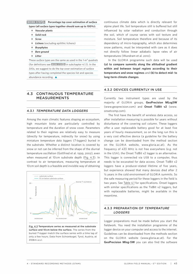
| 43GLORIA FIELD MANUAL – 5TH  EDITION4 - STANDARD RECORDING METHODS (STAM)

 WORK STEP   L   Percentage top cover estimation of surface

types (all surface types together should sum up to 100%):

u Vascular plants

u Solid rock

u Scree

u Lichens (excluding epilithic lichens)

u Bryophytes

u Bare ground

u Litter

These surface types are the same as used in the 1-m² quadrats

(for definitions see  WORK STEP   H  in subchapter 4.1.1). In the

SASs, we suggest to do the top cover estimation of surface

types after having completed the species list and species

abundance recording. s

4.3 CONTINUOUS TEMPERATURE MEASUREMENTS

4.3.1 TEMPERATURE DATA LOGGERS

Among the main climatic features shaping an ecosystem, high mountain biota are particularly controlled by temperature and the duration of snow cover. Parameters related to their regimes are relatively easy to measure (directly for temperature, indirectly for snow) by using miniature temperature data loggers (T-loggers) buried in the substrate. Whether a distinct location is covered by snow or not can be inferred from the shape of the diurnal temperature oscillation (Gottfried et al. 1999, 2002), even when measured at 10 cm substrate depth (Fig.  4.3). In contrast to air temperature, measuring temperature at 10 cm soil depth is a feasible and invisible way of obtaining

continuous climate data which is directly relevant for alpine plant life. Soil temperature still is buffered but still influenced by solar radiation and conduction through the soil, which of course varies with soil texture and moisture. Soil temperature therefore and because of its dependency of micro-topography, which also determines snow patterns, must be interpreted with care as it does not directly follow linear adiabatic lapse rates of air temperatures (Wundram et al. 2010).

In the GLORIA programme such data will be used (a) to compare summits along the altitudinal gradient within and between target regions according to their temperature and snow regimes and (b) to detect mid- to long-term climate changes.

4.3.2 DEVICES CURRENTLY IN USE

Currently two instrument types are used by the majority of GLORIA groups, GeoPrecision MLog5W ( www.geoprecision.com) and Onset TidBit v2 (www.onsetcomp.com).

The first have the benefit of wireless data access, so after installation measuring is possible for years without disturbance of the covering soil column. These loggers offer a user replaceable battery good for at least five years of hourly measurement, so on the long run this is a very cost effective device (a guideline for the battery change can be downloaded from the method section on the GLORIA website, www.gloria.ac.at). As the frequency of 433 MHz is not free everywhere (e.g. not in the USA), the Onset TidBit v2 logger is an alternative. This logger is connected via USB to a computer, thus needs to be excavated for data access. Onset TidBit v2 loggers have a producer-stated lifetime of five years, but experience showed that many devices died after 2 ½ years in the cold environment of GLORIA summits. So the safe measuring period for these loggers in the field is two years. See Table 4.1 for specifications. Onset loggers with similar specifications as the TidBit v2 loggers, but with replaceable batteries, might be available in the meantime.

4.3.3 PREPARATION OF TEMPERATURE LOGGERS

Logger preparations must be made before you start the fieldwork. You need the installation programme of the logger device on your computer and access to the internet. Guidelines can be downloaded from the methods section on the GLORIA website (www.gloria.ac.at). For the GeoPrecision Mlog-5W you can also find the software

diurnal T oscillation

snowcover snowcover

1 day

substrate surface10 cm below substrate surface

no snowcover

Tem

pera

ture

20

10

0

Fig. 4.3 Temperature series as measured at the substrate surface and 10 cm below the surface. The series from the buried T-logger match the surface series with a time lag of only a few hours. Data from Schrankogel, Tyrol, Austria, at 3108 m a.s.l.

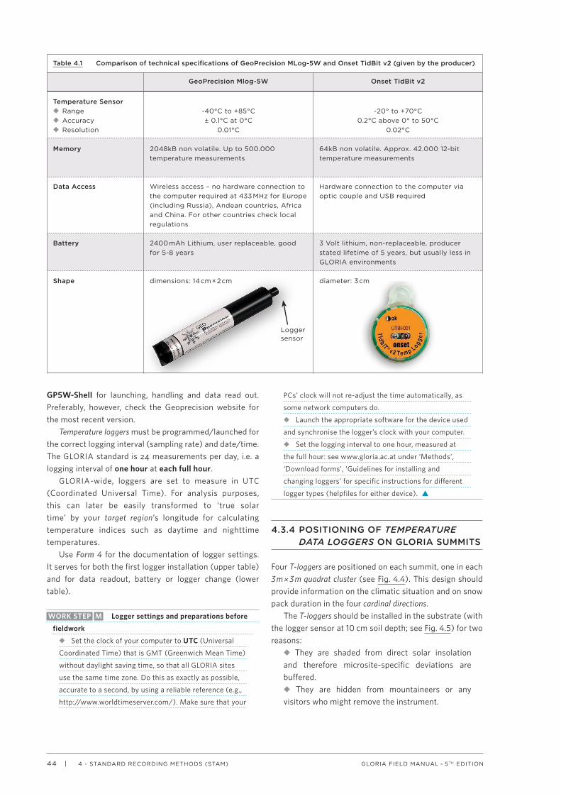
44 | GLORIA FIELD MANUAL – 5TH  EDITION4 - STANDARD RECORDING METHODS (STAM)

GP5W-Shell for launching, handling and data read out. Preferably, however, check the Geoprecision website for the most recent version.

Temperature loggers must be programmed/launched for the correct logging interval (sampling rate) and date/time. The GLORIA standard is 24 measurements per day, i.e. a logging interval of one hour at each full hour.

GLORIA-wide, loggers are set to measure in UTC (Coordinated Universal Time). For analysis purposes, this can later be easily transformed to ‘true solar time’ by your target region’s longitude for calculating temperature indices such as daytime and nighttime temperatures.

Use Form 4 for the documentation of logger settings. It serves for both the first logger installation (upper table) and for data readout, battery or logger change (lower table).

 WORK STEP   M   Logger settings and preparations before

fieldwork

u Set the clock of your computer to UTC (Universal

Coordinated Time) that is GMT (Greenwich Mean Time)

without daylight saving time, so that all GLORIA sites

use the same time zone. Do this as exactly as possible,

accurate to a second, by using a reliable reference (e.g.,

http://www.worldtimeserver.com/). Make sure that your

PCs’ clock will not re-adjust the time automatically, as

some network computers do.

u Launch the appropriate software for the device used

and synchronise the logger’s clock with your computer.

u Set the logging interval to one hour, measured at

the full hour: see www.gloria.ac.at under ‘Methods’,

‘Download forms’, ‘Guidelines for installing and

changing loggers’ for specific instructions for different

logger types (helpfiles for either device). s

4.3.4 POSITIONING OF TEMPERATURE DATA LOGGERS ON GLORIA SUMMITS

Four T-loggers are positioned on each summit, one in each 3 m × 3 m quadrat cluster (see Fig. 4.4). This design should provide information on the climatic situation and on snow pack duration in the four cardinal directions.

The T-loggers should be installed in the substrate (with the logger sensor at 10 cm soil depth; see Fig. 4.5) for two reasons:

u They are shaded from direct solar insolation and therefore microsite-specific deviations are buffered.u They are hidden from mountaineers or any visitors who might remove the instrument.

Table 4.1 Comparison of technical specifications of GeoPrecision MLog-5W and Onset TidBit v2 (given by the producer)

GeoPrecision Mlog-5W Onset TidBit v2

Temperature Sensoru Rangeu Accuracyu Resolution

-40°C to +85°C± 0.1°C at 0°C

0.01°C

-20° to +70°C0.2°C above 0° to 50°C

0.02°C

Memory 2048kB non volatile. Up to 500.000 temperature measurements

64kB non volatile. Approx. 42.000 12-bit temperature measurements

Data Access Wireless access – no hardware connection to the computer required at 433 MHz for Europe (including Russia), Andean countries, Africa and China. For other countries check local regulations

Hardware connection to the computer via optic couple and USB required

Battery 2400 mAh Lithium, user replaceable, good for 5-8 years

3 Volt lithium, non-replaceable, producer stated lifetime of 5 years, but usually less in GLORIA environments

Shape dimensions: 14 cm × 2 cm diameter: 3 cm

Logger sensor

| 45GLORIA FIELD MANUAL – 5TH  EDITION4 - STANDARD RECORDING METHODS (STAM)

 WORK STEP   N   Positioning and photo documentation of

the data loggers

u Within each 3 m × 3 m quadrat cluster, look for a

suitable logger position within the central quadrat (e.g.

N22) where a logger can be buried 10 cm below the

substrate surface. This position should represent an

average surface and habitat situation of the 3 m × 3 m

area. Therefore, avoid deviating locations, such as, e.g.

directly aside a protruding rock or a boulder. Where

the logger cannot be positioned in the central quadrat,

choose a proper position in another quadrat (e.g. in the

quadrats N12, N21, N23, or N32, for quadrat numbers

compare Fig. 4.1) but never put a logger inside the four

corner quadrats where you do the species recordings.

››  Generally, the logger position should represent

the average microclimate situation of the 3 m × 3 m

quadrat cluster.

u Dig a small, 10-cm-deep hole and take care not to

destroy the surrounding substrate texture.

u Write the logger position and installation year onto

the logger body: the scheme CC-TTT-SSS-QQQ-YYYY

(i.e., CC, country; TTT, target region; SSS, summit; QQQ,

quadrat; YYYY, year). Use a waterproof marker for

writing on the logger.

u Enter the quadrat code, logger serial number, and

logger type into the protocol (Form 4).

u When using Onset Tidbit loggers, fix a short string

of approx. 10 cm length onto the T-logger – this will help

to find the device again in the future. This may also be

useful for Geoprecision loggers.

u Put the logger into the hole. Make sure that

the logger’s sensor (see Fig. 4.5, lower left) lies

approximately 10 cm below the surface level.

u Measure the distance (in metres with two decimal

places) from the centre of the logger’s hole to the lower

Fig. 4.4 T-logger positioning. In each cardinal direction of a summit site, one T-logger is positioned within the central quadrat of the 3 m × 3 m quadrat cluster (see  WORK STEP   N  for alternative logger positioning, if necessary). See Box 6.1 for the full-length-loggercodes.

N11

N13

N33

N31

S11

S13S33

S31

E11

E13

E33E31

W11W13

W33

W31

T-logger:CC/TTT/SSS/S22/YYYY

T-logger:CC/TTT/SSS/N22/YYYY

T-logger:CC/TTT/SSS/E22/YYYY

T-logger:CC/TTT/SSS/W22/YYYY

HSP

Fig. 4.5 Installation of a temperature logger. Upper left, the logger may be positioned horizontally or obliquely (as shown in the example), but the sensor always must be at 10 cm below surface and the uppermost parts should be covered by several centimetres of substrate material. Lower left, logger position uncovered, lower right, logger covered with soil material (gardening trowel points to the position of the sensor). Upper right: Example of a logger position in the center quadrat of a 3 m × 3 m grid with measurement lines to the lower corner points of the 3 m × 3 m quadrat cluster.

S11 S31

S13 S33

p-S13 p-S33

p5m-S11 p5m-S31

(S23)

(S22)

(S21)

(S12) (S32) Towards the H

SP

(Row 1)

(Row 2)

(Row 3)

(Column 1)

(Column 2)

(Column 3)

Dist-11 Dist-31Example for logger position

10cm

Logger sensor

Surface

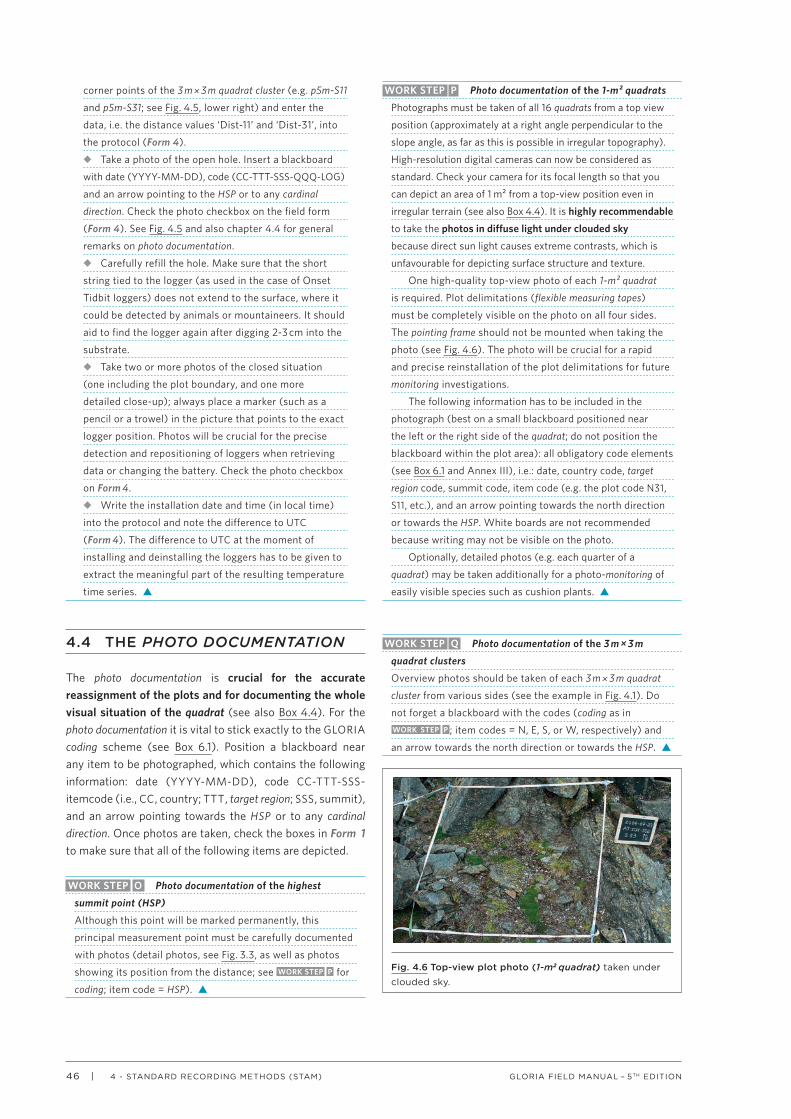
46 | GLORIA FIELD MANUAL – 5TH  EDITION4 - STANDARD RECORDING METHODS (STAM)

corner points of the 3 m × 3 m quadrat cluster (e.g. p5m-S11

and p5m-S31; see Fig. 4.5, lower right) and enter the

data, i.e. the distance values ‘Dist-11’ and ‘Dist-31’, into

the protocol (Form 4).

u Take a photo of the open hole. Insert a blackboard

with date (YYYY-MM-DD), code (CC-TTT-SSS-QQQ-LOG)

and an arrow pointing to the HSP or to any cardinal

direction. Check the photo checkbox on the field form

(Form 4). See Fig. 4.5 and also chapter 4.4 for general

remarks on photo documentation.

u Carefully refill the hole. Make sure that the short

string tied to the logger (as used in the case of Onset

Tidbit loggers) does not extend to the surface, where it

could be detected by animals or mountaineers. It should

aid to find the logger again after digging 2-3 cm into the

substrate.

u Take two or more photos of the closed situation

(one including the plot boundary, and one more

detailed close-up); always place a marker (such as a

pencil or a trowel) in the picture that points to the exact

logger position. Photos will be crucial for the precise

detection and repositioning of loggers when retrieving

data or changing the battery. Check the photo checkbox

on Form 4.

u Write the installation date and time (in local time)

into the protocol and note the difference to UTC

(Form 4). The difference to UTC at the moment of

installing and deinstalling the loggers has to be given to

extract the meaningful part of the resulting temperature

time series. s

4.4 THE PHOTO DOCUMENTATION

The photo documentation is crucial for the accurate reassignment of the plots and for documenting the whole visual situation of the quadrat (see also Box 4.4). For the photo documentation it is vital to stick exactly to the GLORIA coding scheme (see Box  6.1). Position a blackboard near any item to be photographed, which contains the following information: date (YYYY-MM-DD), code CC-TTT-SSS-itemcode (i.e., CC, country; TTT, target region; SSS, summit), and an arrow pointing towards the HSP or to any cardinal direction. Once photos are taken, check the boxes in Form  1 to make sure that all of the following items are depicted.

 WORK STEP   O   Photo documentation of the highest

summit point (HSP)

Although this point will be marked permanently, this

principal measurement point must be carefully documented

with photos (detail photos, see Fig. 3.3, as well as photos

showing its position from the distance; see  WORK STEP   P  for

coding; item code = HSP). s

 WORK STEP   P   Photo documentation of the 1-m² quadrats

Photographs must be taken of all 16 quadrats from a top view

position (approximately at a right angle perpendicular to the

slope angle, as far as this is possible in irregular topography).

High-resolution digital cameras can now be considered as

standard. Check your camera for its focal length so that you

can depict an area of 1 m² from a top-view position even in

irregular terrain (see also Box 4.4). It is highly recommendable

to take the photos in diffuse light under clouded sky

because direct sun light causes extreme contrasts, which is

unfavourable for depicting surface structure and texture.

One high-quality top-view photo of each 1-m² quadrat

is required. Plot delimitations (flexible measuring tapes)

must be completely visible on the photo on all four sides.

The pointing frame should not be mounted when taking the

photo (see Fig. 4.6). The photo will be crucial for a rapid

and precise reinstallation of the plot delimitations for future

monitoring investigations.

The following information has to be included in the

photograph (best on a small blackboard positioned near

the left or the right side of the quadrat; do not position the

blackboard within the plot area): all obligatory code elements

(see Box 6.1 and Annex III), i.e.: date, country code, target

region code, summit code, item code (e.g. the plot code N31,

S11, etc.), and an arrow pointing towards the north direction

or towards the HSP. White boards are not recommended

because writing may not be visible on the photo.

Optionally, detailed photos (e.g. each quarter of a

quadrat) may be taken additionally for a photo-monitoring of

easily visible species such as cushion plants. s

 WORK STEP   Q   Photo documentation of the 3 m × 3 m

quadrat clusters

Overview photos should be taken of each 3 m × 3 m quadrat

cluster from various sides (see the example in Fig. 4.1). Do

not forget a blackboard with the codes (coding as in  WORK  STEP   P ; item codes = N, E, S, or W, respectively) and

an arrow towards the north direction or towards the HSP. s

Fig. 4.6 Top-view plot photo (1-m2 quadrat) taken under

clouded sky.

| 47GLORIA FIELD MANUAL – 5TH  EDITION4 - STANDARD RECORDING METHODS (STAM)

 WORK STEP   R   Photo documentation of the corner points

of the summit area sections

The following items have to be documented:

u The highest summit point (HSP) made in  WORK STEP   O .

u The four 10-m points: coding as in  WORK STEP   P ;

item codes = p10m-N, p10m-E, p10m-S, and p10m-W,

respectively.

u The eight summit area points in the intermediate

directions: coding as in  WORK STEP   P ; item codes = pNE-5,

pNE-10, pSE-5, pSE-10, pSW-5, pSW-10, pNW-5, and

pNW-10, respectively.

The corner points should be marked with a signal

stick or rod (1 to 1.5 m length) to make them visible on

the photo: the small aluminium tubes and/or stones

used as permanent markers may be insufficient for this

purpose (see Fig. 4.7). A detailed photo as well as an

overview photo should be taken of each point, always

with the blackboard included with the relevant code,

date and an arrow pointing towards the north

direction. s

 WORK STEP   S   Photo documentation of the entire summit

Take a photo of the summit (e.g. from a neighbouring

hump in the ridge or from an opposite place at the other

side of a valley if distances are not too large) to show

the geomorphologic shape and the general situation (see

examples in Fig. 2.2). Use a blackboard including the codes

if possible (use SU-OV as item code; see Annex III for

codes). Do not forget the arrow towards the north or any

other cardinal direction. s

OPTIONAL  WORK STEP   T   Other detail photos

If you think that it might be important to do more detailed

photo documentation, e.g. of the position of intersection

lines and other lines, such photos are highly appreciable.

For coding of these details use the next-lying obligatory

item (compare  WORK STEPS     O  -   R ). If this item is not

seen on the photo view, add an arrow on the blackboard

pointing from the written code in the direction of the item

to which the code belongs. Also do not forget the north or

HSP arrow. s

Fig. 4.7 A corner point of a summit area section. The 10 m-point (p10m-W) on Pico del Tosal Cartujo (Sierra Nevada/Spain, 3150 m a.s.l.) is marked with a signal rod for photo documentation.

BOX 4.4 PHOTO DOCUMENTATION – GENERAL CONSIDERATIONS

Photographs or paper copies of the photos have prov-en to be the most important reference for a fast and accurate reassignment of plots.

u Photos allow the plots to be re-established without repeating the time-consuming mea-surements.u Moreover, photos are much more than instruments to relocate the plots. They docu-ment the entire v isual situation of the perma-nent plots in ways that are of great compara-tive value, e.g. for tracing of local distribution patterns of particular species over many years or decades.u For both the above reasons, all photos must be retaken at each monitoring cycle.u The photo documentation should be done carefully and, whenever possible, under cloud-ed sky to avoid hard contrasts.u Use the camera’s high-resolution adjust-ment.u Ensure that each photograph is labelled with its full-length photo code (see Box 6.1) written on a blackboard which has to be included in the picture wherever applicable, but put the board outside of the 1-m² plot.u Mark the »photo checkboxes« in the Forms 1 and 4 to control whether all obligatory photos were taken.u Store your photos using consistent labels. See chapter 6.3 and Annex III and use the provided software (GPDM, GLORIA Photo Data Management) for standardised names of your JPEG photo files.

FOCAL LENGTH OF LENSFor depicting the full 1-m² quadrats a wide-angle lens is required. Please check before fieldwork if your camera is suitable for depicting an area of 1 m² from a top-view position in different terrain conditions – also check if this fits to the body size of the person in charge of the photo documentation. Photos of the corner points and loggers may be taken with a standard or any appropri-ate focal length.

48 | GLORIA FIELD MANUAL – 5TH  EDITION4 - STANDARD RECORDING METHODS (STAM)

PHOTOS AND MEASUREMENT DATA FOR THE REASSIGNMENT OF PLOTS

The fast and accurate reassignment (re-establishing) of the plots for monitoring investigations will usually be accomplished only by using printed photographs of the quadrats and the corner points of the summit area sections. Thus, there is usually no need to repeat the time-consum-ing measuring work, described in chapter 3.3, at the beginning of the resurvey.

Measurements of plot positions made during the first site setup are nevertheless essential for the following purposes:

u The determination of exact geographic directions and the 5-m and 10-m levels.u For the re-establishment of plots in cases where this is not possible only by photographs. This may be the case, e.g., in uniform and closed grassland or in vegetation dominated by taller growing forbs. Unexpectedly rapid vegetation changes, e.g., through shrub encroachment, may be a further reason to repeat the mea-surements of plot corner points. u Re-establishing after severe disturbance events. This can lead to the loss of the previous habitat or to a pronounced relocation of the vegetation patch. In such cases, re-measure ments may be necessary as well as a careful documentation of the disturbance. Plots exposed to more continuous slow-pace disturbance, such as through solifluction that may not strongly and rapidly distort the habitat and vegetation patterns, usually should be detectable and reassignable just with the photo.u A detailed outline of the actual summit area and plot positions can be produced from the measurement data. Printouts of outline sketches can aid to find the corner points of the summit area sections, but also can help to evaluate your previous measure-ments. For example, implausible shapes of summit area sections should be checked again (re- measured) in the field.

u Finally, measurements enable the calculation of the area size of each summit area section for subsequent data analysis.

RESURVEY INTERVALS AND TIMING

Monitoring cycles are performed at intervals of five to ten years. Globally fixed or concerted intervals might be desirable but are difficult to arrange due to logistic and financial con-straints. Starting dates of baseline investigations vary and the expansion of the GLORIA network through new target regions is still ongoing at a rather steady, unabated pace. There-fore and because of r egional and northern/ southern hemisphere differ-ences, and of tropical peculiarities, a worldwide coordination of monitoring cycles seems to be impracticable. Funding uncertainties and time constraints are a further reason for varying resurvey intervals. For example, the first broad-scale re- recording campaign on the European level was conducted in 2008, seven years after the baseline investigation and the second is planned for 2015. Yet, a number of sites in North America and in Australasia were resurveyed after five years. Shorter intervals of monitoring cycles, such as every year, might be of interest for determining inter-annual variability which, however, is expected to be rather low due to the long-lived nature of the large majority of alpine plant species. Besides the consider-able extra effort and expense, short intervals can also cause interfering disturbance due to increased trampling by the investigators.

More important than internation-ally concerted monitoring cycles is a good timing of the resurvey campaign within the growing season. Resurveys should be conducted at the same date or period as the baseline inves-tigation, which, in seasonal climates, should be around the mid-growing season. Particularly deviating late or early onsets of the growing season, however, should be taken into consid-eration when you plan your resurvey campaign. Generally, it is advisable to start not too early in the season, when generative or even vegetative

parts of species may not yet be well developed.

RESURVEY PROCEDURE

At resurveys, the fieldwork procedure is principally the same as at the base-line investigation. The only difference is that you usually do not need to re-measure distances and compass angles from the HSP to the plot corner points. Print all your photos of the quadrats and corner points for the exact re-establishments of plots, but also your measurement protocol for the case that positions cannot be properly identified with the photo (e.g. in taller-growing dense vegetation). Photos, nevertheless, are essential for precisely re-establishing the 1-m² quadrats and the delimitations of the summit area sections.

All standard recording procedures in the 1-m² quadrats and in the summit area sections must be repeated ‘blind’, i.e. without any aid of old data in order to keep an unbiased compa-rability of, e.g. species occurrences, cover values or turnovers. Neither the previous plot data such as species lists or cover values, nor photos of the quadrats are used during resur-veys. Apart from this, however, the resurvey team, particularly if con-sisting of new members, should be familiar with all species occurring in the region, and therefore, the overall species list of your summit sites and previous herbarium materials could be of much help. Previous species lists of quadrats and SASs only can be used after having completed recording, e.g. to aid the identification of doubtful species.

In summary, use the same mate-rials, equipment and blank sampling forms for your resurvey campaign. For re-establishing the plots, bring print-outs of all photos and the measure-ment data of plot positions including outline sketches of the summit sites.

For reading out temperature data and for servicing your data loggers, bring the logger installation data (all data you entered in Form 4) and, if you have to dig out loggers for readout, battery change or replacement, the photos of the logger installation, some spare loggers and service equipment are needed.

BOX 4.5 CONSIDERATIONS FOR FUTURE REASSIGNMENTS AND RESURVEYS

| 49GLORIA FIELD MANUAL – 5TH  EDITION4 - STANDARD RECORDING METHODS (STAM)

4.5 REMOVAL OF PLOT DELIMI - TATIONS AND CONSIDERATIONS FOR FUTURE REASSIGNMENTS AND RESURVEYS

Given the multi-year intervals between resurveys and the long-term dimension of GLORIA summit observations, any non-durable parts of plot delimitations are to be removed before you leave the summit site. Only small aluminium tubes (or other appropriate markings) at the plot corners and the buried temperature data loggers remain at the site.

Box 4.5 gives a brief view on what will be needed for future repetitions of your summit work.

 WORK STEP   U   Removal of plot delimitations

Before you remove any delimitation, check Forms 1 and 4

to ensure that all plots/items have been documented with

photographs and check if recording is completed in all plots.

The 3 m × 3 m grids and all strings delimiting the summit area

sections have to be removed after all recording and the photo

documentation is finalised. s

4.6 GENERAL INFORMATION ON THE TARGET REGION

This chapter focuses on information concerning the entire target region, i.e. the area within which all four summit sites are situated. The overall altitudinal zonation of vegetation belts, bedrock material, and the land use history should be described. We suggest to fill in the respective sampling

form when you are still in the field, as far as possible, but it might be completed later on, e.g. if additional information on land use history is required.

See the sampling sheet Form 0.

 WORK STEP   V   Provide information about the

target region

u Estimates of the altitudinal position in metres above

sea level of:

v the forest line (i.e. the line where closed

forests end, as seen from the distance); enter

both the potential natural and the current forest

line.

v the treeline (i.e. the line where closed groups

of trees taller than 3 m end); enter both the

potential natural and the current treeline.

v the alpine-nival ecotone (i.e. the transition

between the upper alpine and the nival zone) in

your target region.

v Where required, make comments on these

major ecotonal zones, e.g. deviations from the

average altitude and make a note if a boundary

line does not exist in the target region and on any

reason for its absence.

u Describe the bedrock material of the summit sites of

the target region, which should be consistent throughout

the four summits, i.e. consistent regarding the

influence of the bedrock on the species composition. In

addition, make a rough estimate on the average soil pH

(e.g. acidic: <4.5, intermediate: 4.5-6.5, neutral/alkaline:

>6.5).

As mentioned in subchapter 2.2.2, human trampling, grazing by livestock or other anthropogenic influences may mask possible climate-related changes. Thus, sites being strongly affected by human land use should be avoided, e.g. if grazing-indicator species are common or dominant, tracks and droppings of livestock are obvious. In many mountain regions, however, it is difficult to find graz-ing-free, ‘pristine’ summit habitats. Therefore, it is important to take land use impacts and particularly any pronounced changes in land use practices under consideration when analysing climate-induced vegetation changes. A difficulty in recording land use features is that these may be very region-specific and changes in land use practices may not be easy to

detect. Information on such land use changes, however, appears to be more relevant than an indication of the current land use intensity. Moderate traditional grazing over centuries is expected to produce less background noise than pronounced changes, e.g. within the past 50 or 100 years. A high grazing intensity, further, may be assessed by particular species that indicate grazing impacts.

Systematic field recording of anthropogenic factors that may im-pact alpine vegetation and species composition is not a core focus of the standard protocol.

For summit area sections (Form 3), however, comments on livestock grazing impacts such as occurrence of dropping, traces of trampling, and of browsing damage are requested.

The supplementary sub-plot frequency counts in 1-m² quadrats include record-ing of these grazing effects in 100 subplots (Form 5-S, chapter 5.1.2).

Comments on the land use history in relation to the current situation are requested on Form 0 for the general region description. Comments should be based on re-gional historical records or reliable local informants and should consider, depending on the region, a range of possible factors such as pastoralism, burning practices, hunting, agricul-ture, tourism, mining, or any other relevant more specific influence. Attempts on a systematic recording and assessment of land use factors, along with socio-economic aspects in GLORIA regions are outlined in chapter 7.6.

BOX 4.6 HUMAN LAND USE AND GRAZING IMPACTS

50 | GLORIA FIELD MANUAL – 5TH  EDITION4 - STANDARD RECORDING METHODS (STAM)

u Provide a short description of the target region,

particularly regarding the land use history and the

current land use situation. Indicate if the situation is

pristine or in a near natural state. If this is not the case,

indicate what kind of human land use has or had an

impact on the present vegetation. Wherever possible,

comment on the extent of land use impacts and provide

information on the long-term and recent land use

history. Of particular interest are more recent changes

(e.g. within the past 50 years) in the grazing/land use

regime that may still continue to have an effect on

current vegetation changes (see also Box 4.6).

u Enter the vegetation zone or ecotone in which

the summit is located: only the following entries are

possible: treeline ecotone, lower alpine, lower/upper

alpine ecotone, upper alpine, alpine-nival ecotone,

nival; see Box 2.1 and Nagy and Grabherr (2009) for

definitions.

u Make comments on the situation of the particular

summit if the above zonation scheme is not properly

applicable and describe the deviations. Further,

comment on any other pronounced deviation from an

‘ideal’ standard summit situation (compare chapter 2.2

on summit selection and Box 2.1 on definitions of

vegetation zones). s

| 51GLORIA FIELD MANUAL – 5TH  EDITION5 - SUPPLEMENTARY SAMPLING DESIGNS AND RECORDING METHODS (SUPM)

Several supplementary methods were applied in a subset of GLORIA summit sites and are considered as an extension of the standard Multi-Summit Approach. All these supplementary methods described here are directly related to the standard GLORIA sampling design. They follow various focuses, such as additional recording methods (subplot-frequency counts in 1-m² quadrats, species cover recording in SASs, pointing in 10 m × 10 m squares), an extended number of 1-m² quadrats per summit site in order to enhance the power of statistical change detection, and/or the inclusion of organism groups like bryophytes and lichens. Some of these further recording procedures were previously regarded as GLORIA standard methods and were recently shifted to the optional level.

Whenever you plan to apply supplementary methods on your monitoring summit, consider that this may be a source of additional disturbance through enhanced trampling impacts. This particularly applies for sites with steeper terrain and/or unstable scree habitats or for disturbance-sensitive vegetation such a plant communities dominated by cryptogam species. Further, consider the additional time effort that should not go on the expense of a careful completion of the standard approach.

CONTENT OVERVIEW

5.1 Supplementary recording in 1-m² quadrats  525.1.1 Recording of bryophytes and lichens in 1-m² quadrats  525.1.2 Subplot-frequency counts in the 1-m² quadrats  525.1.3 Supplementary 1-m² quadrats at the 10-m level  53

5.2 Supplementary recording in summit area sections  545.2.1 Recording of bryophytes and lichens in summit area sections  545.2.2 Recording of species cover in summit area sections with Point and Flexible Area (PAF) sampling method  54

5.3 Line-pointing and species recording in 10 m × 10 m squares  565.3.1 Line-pointing of vascular plants in 10 m × 10 m squares  575.3.2 Recording of additional species in 10 m × 10 m squares  58

5 SUPPLEMENTARY SAMPLING DESIGNS AND RECORDING METHODS (SUPM)

52 | GLORIA FIELD MANUAL – 5TH  EDITION5 - SUPPLEMENTARY SAMPLING DESIGNS AND RECORDING METHODS (SUPM)

5.1 SUPPLEMENTARY RECORDING IN 1-m2 QUADRATS

5.1.1 RECORDING OF BRYOPHYTES AND LICHENS IN 1-m2 QUADRATS

Bryophytes and lichens are each considered as entire organism group in the top cover sampling of the obligatory standard recording procedure (chapter  4). Recording of cryptogams (bryophytes and lichens) on a species level, however, is only treated as an optional supplementary activity, because of the following considerations: Recording of cryptogams on the species level often is hampered by the very low number of experts; bryologists and lichenologists who may be able to identify the bulk of species already in the field may not be available. Additionally, the smaller size of individuals and, therefore, their often large numbers, require considerable extra time or a larger team. The resulting increase of the trampling impact has to be taken into account.

The decision of doing lichen and bryophyte species recordings in the 1-m² quadrats, further, depends on their regional importance in terms of species numbers, biomass and vegetation cover.

Note: For cryptogam species, the same field sheets can be used as for vascular plants (Form 2 for recording in 1-m² quadrats) for visual cover estimation and pointing.

5.1.2 SUBPLOT-FREQUENCY COUNTS IN THE 1-m2 QUADRATS

Subplot-frequency counts, previously a standard method of the Multi-Summit Approach, is now only considered as an optional supplementary. The main reason for this is the extensive time and labour required for this method and the associated trampling impact. In a global context, where many sites lie in remote areas, the time-consuming method hardly can be considered as a feasible component of the basic approach.

Frequency counts of vascular plant species (and of obvious grazing impacts) are made in all 16 1-m² quadrats. The aim is to detect changes of vegetation patterns on a fine-scaled level (compare Box 5.1).

As a general rule, frequency counting should not be made in those particular quadrats where the grid frame cannot be properly mounted, to avoid inexact results. This can be the case on summits within the treeline ecotone, where small trees or shrubs may occur within the quadrats or in any tall-growing vegetation.

In addition, features indicating the presence of grazing mammals are recorded. Three grazing-related features are distinguished:

u faeces/droppings, u browsing damage (clipped shoots, leaves and/or inflorescences), and u trampling (e.g. hoof marks, foot prints, broken lichens, and/or scuffed tussocks).

For the sampling sheet see Form 5-S in Annex II.

 RECORDING PROCEDURE u A wooden (or aluminium) grid frame with 100 cells of

0.1 m × 0.1 m, delimited by thin white strings (see Fig. 5.1

and Fig. AI.2 in Annex I for construction details; note that

covering differs from the pointing frame) will be used for

the frequency counts.

u In each cell, presence of vascular plant species and

of grazing features will be recorded. All species seen

inside a grid cell must be recorded as present for that

particular cell. Thus, a species is considered as present

when plant parts can be seen within the boundary

strings of the 0.1 m × 0.1 m grid cell, regardless of where it

is rooted.

Note: Recording must always be done perpendicular

to the slope angle (i.e. perpendicular to the grid

frame plane). Particular care should be taken on

uneven relief, where the grid frame cannot be

positioned flat on the surface.

u Take a photo of the plot with the grid frame

mounted so that it can be properly reinstalled at

resurveys. s

BOX 5.1 FREQUENCY COUNTS – GENERAL CONSIDERATIONS

Records on the presence of species obtained by the 100-cells grid frame are used to monitor changes in vegetation patterns on a fine-scaled level. An accurate relocation of the grid frame at each successive record-ing is a precondition for reliable monitoring records. Therefore, when you apply subplot frequency record-ing take an additional photo of the 1-m² quadrat with the grid frame mounted.

Subplot frequency counts are sensitive for clustered species distribution patterns (e.g. for cushion plants and compact tussocks) and less so for scattered or highly dispersed occurrences. Time-consuming counts of species with large numbers of small-sized and dispersed individuals (as this is typical for many bryo-phyte but also for a number of vascular plant species) usually result in high frequency values, even if their species cover is low. See Friedmann et al. (2011) for a comparison of subplot frequency counts with visual cover estimation.

| 53GLORIA FIELD MANUAL – 5TH  EDITION5 - SUPPLEMENTARY SAMPLING DESIGNS AND RECORDING METHODS (SUPM)

5.1.3 SUPPLEMENTARY 1-m2 QUADRATS AT THE 10-m LEVEL

Jean-Paul Theurillat ¹,² & Pascal Vittoz³   

1 | Centre Alpien de Phytogeographie, Fondation J.-M. Aubert, Champex-Lac, Switzerland; 2 | University of Geneva, Section of Biology, Switzerland; 3 | University of Lausanne, Department of Ecology and Evolution, Switzerland

A larger number of 1-m² quadrats on each GLORIA summit would be desirable in order to enhance the statistical power for the detection of small changes. This is especially of interest for assessing slight shifts of species cover on a local to regional level or when focusing on changes of individual species. The consequences of the increased effort (more time or more observers are required), however, must be carefully considered in alpine environments, where the peak growing season usually is short and often interrupted by adverse weather conditions. Doubling the number of plots would not only mean twice as much time for species recording, but also for the plot setup and photo documentation. A team of four persons, therefore, may not be able to complete these supplementary quadrats within one growing season. Establishing additional plots should certainly not go on the expense of the required standard procedures. Supplementary quadrats, thus, should only be established after all standard procedures in the obligatory 16 quadrats and in the eight summit area sections were carefully completed. More 1-m² quadrats, further, would mean more disturbance caused by the investigators.

SAMPLING DESIGN  AND  RECORDING PROCEDURE 

FOR  SUPPLEMENTARY PLOTS 

u Positioning: Supplementary plots are also arranged

in a 3 m × 3 m grid, where the four corner quadrats should

be used as permanent plots. In each cardinal direction,

one supplementary 3 m × 3 m grid should be placed at

the 10-m level below the HSP and should be aligned

parallel to the slope. The lower line of the 3 m × 3 m

grid lies somewhat above the respective p10m-point

(i.e. the 10-m points of each cardinal direction) so that

the lower corner points of the 3 m × 3 m grid touch the

lower boundary lines of the 10-m summit area section

(see Fig. 5.2). The sharper the angle of the lower

SAS boundary lines, the greater is the distance of the

3 m × 3 m grid from the 10-m point.

u Coding: The supplementary quadrats must have a

3-character alphanumeric code. This is necessary to enable

administrative compatibility with the coding for standard

plots in the central GLORIA database. The coding scheme:

e.g. Na1, Na2,…Wa4; N, E, S, or W stands for the respective

cardinal direction, a is the indication as a supplementary

Row 1

Row 2

Row 3

Row 4

Row 5

Row 6

Row 7

Row 8

Row 9

Row 0

Colum

n 1

Colum

n 2

Colum

n 3

Colum

n 4

Colum

n 5

Colum

n 6

Colum

n 7

Colum

n 8

Colum

n 9

Colum

n 0

Quadrat size: 1 m

Towards the H

SP

Fig. 5.1 Grid frame for species frequency counts. Upper, grid frame mounted on a plot; lower, scheme of the 1 m × 1 m grid frame, subdivided into 0.1 m × 0.1 m cells for recording species presence and grazing-related features in each cell. Please note that the frequency grid frame is different from that used for point-framing (compare Fig. 4.2).

Fig. 5.2 Positions of 16 supplementary quadrats. Four in each cardinal direction near the 10-m level and arranged in 3 m × 3 m grids.

10 m

1m 2m

3m4m

5m6m

7m

8m

9m

10m

N

HSP

54 | GLORIA FIELD MANUAL – 5TH  EDITION5 - SUPPLEMENTARY SAMPLING DESIGNS AND RECORDING METHODS (SUPM)

plot, 1, 2, 3, or 4 the plot number in clockwise order,

starting with the lower left quadrat (see Fig. 5.3).

u Recording: For species recording in supplementary

quadrats the same methods and procedures are to be

applied as in the obligatory standard quadrats (see

chapter 4.1). s

5.2 SUPPLEMENTARY RECORDING IN SUMMIT AREA SECTIONS

5.2.1 RECORDING OF BRYOPHYTES AND LICHENS IN SUMMIT AREA SECTIONS

See the considerations under 5.1.1.

Note: For cryptogam species recording in summit area sections the same field sheet (Form 3) as for vascular plants can be used. Also estimate the abundance of cryptogam species along the abundance categories described in chapter 4.2.

5.2.2 RECORDING OF SPECIES COVER IN SUMMIT AREA SECTIONS WITH POINT AND FLEXIBLE AREA (PAF) SAMPLING METHOD

Stephan Halloy¹ ,², Mariana Musicante², Mercedes Ibáñez¹ & Karina Yager³

1 | The Nature Conservancy, Santiago, Chile; 2 | Universidad Nacional de Chilecito, Argentina; 3 | NASA Goddard Space Flight Center, Biospheric Sciences Laboratory, Maryland, USA

The obligatory standard recording procedure in summit area sections (SAS) involves a complete species list (all

vascular plant species) and an estimation of species’ abundances by using five verbally defined classes as well as a percentage cover estimates of the main surface types (compare chapter 4.2). This can be done in reasonable time and, thus, most effort can concentrate on capturing all species that occur within one SAS .

More precise data on the area coverage of each species, however, would be preferable in principle if sufficient time and/or observers are available. Data on species cover would allow for more advanced statistical analyses, such as obtaining species-area curves, deriving rank-abundance curves and their respective analyses, as well as the calculation of indices such as the Shannon-Weaver diversity index, equitability, distance to a lognormal fit (ΔL), etc. (see Magurran 1988, Halloy & Barratt 2007); see also the considerations in Box 5.2.

A difficulty in cover estimation in summit area sections, however, is that these recording areas may greatly vary in size (a few 100 m² to several 1000 m²), shape and topography. This complicates a straight-forward and time-saving recording of species cover, particularly in complex mosaics of patchy vegetation and where species richness is high.

There are several approaches on how to determine species cover and the suitability of one or another method depends on the abundance of a species, their growth form and distribution pattern. Therefore, a combined approach using classical point-line intercepts (Scott 1965, Dickinson et al. 1992) as well as a flexible area is suggested here (e.g. Halloy et al. 2011).

 METHODS  AND  RECORDING PROCEDURE 

u Point-line intercepts

The point-line intercept method is used here to measure

the cover of the more common species and of the main

surface types. A 50-m sampling line is established within

the summit area section, randomly positioned across the

centre of the section, e.g. using a 50-m measuring tape.

Every 50 cm along the line, a pointing stick (e.g. a stick

or a knitting needle of 2 mm diameter) is brought down

vertically until it touches the first object, may it be a plant

or soil or rock. In shrubby vegetation, this point may be

above the string. The idea is to consider the first point that

a drop of rain falling vertically would hit. This is the point

that a satellite would ‘see’, and therefore the point that

will be integrated (into the average of much larger pixels)

in the spectral signature of the satellite image (such as

measured with NDVI ratios). The combination of all points

(percentage cover) represents the ‘image’ of the vegetation

as seen from above. For each point of contact, a stroke (or

bar) is marked on the field data sheets (e.g. species A: II,

species B: I, scree: IIII, solid rock: II, bare ground: I, etc.). In

the end we should have 100 strokes on our sampling sheet

to H

SP

South

Sa3

Sa4

Sa2

Sa1

Fig. 5.3 Coding of supplementary quadrats at the 10-m level (here, codes of the southern 3 m × 3 m grid are shown).

| 55GLORIA FIELD MANUAL – 5TH  EDITION5 - SUPPLEMENTARY SAMPLING DESIGNS AND RECORDING METHODS (SUPM)

for the 100 sampled points. The proportion of each item in

those 100 points represents its abundance or percentage

cover (e.g. species A: 2%, species B: 1%, scree: 4%, etc.).

In large SASs and/or in those with discontinuous

vegetation, the length of the line can vary or additional

lines may be placed, but consider this when calculating

the percentage cover from the number of hits (e.g. when

you have 300 points and species A was touched 21

times, its resulting cover would then be 7%). In smaller

sections, it is quite appropriate to do several shorter

segments, e.g. 12 m, 16 m, 15 m, 7 m, as long as the

minimum 100 points are achieved.

Measuring cover by point-line intercepts is simple and

may take less than a half hour per SAS or less than one

As there is considerable debate and misunderstanding in regards to field methods of quantifying vegetation, it is important to clarify a few points – particularly in regards to time and search effort versus precision of re-sults. There is no way around the fact that whatever way you write down the numbers, you will first have to observe the vegetation. Once you have observed, the rest happens in your mind. Most methods are simply mental crutches to help make sense of what you have observed. One could of course in theory measure every single plant and calculate abundance and cover. As this is impractical, both in terms of field time and effort, as well as in environmental damage (trampling), all other methods in-corporate visual best estimates. We have a choice of a quick estimate of the most abundant species, or delving deeper and trying to find all species. Because GLORIA is about understand-ing changes, we accept the additional time and effort to attempt to find all species (e.g. see above and Box 4.1 for 1-m² quadrats). Since we assume the necessary time to find all species we then have some choices of how we mind-process the data without losing additional field-time.

Continuous versus categoricalEstimates of species cover can be reported as continuous numbers (e.g. measures of area or percentage of area, 1, 4, 6, 25, 50 etc.), or as cate-gories (e.g. ordinal, as in  WORK STEP   K , chapter 4.2; or a, b, c, where a=cover of 1−7, b=8 to 15, etc.). Supporters of categorical reporting argue for (1) saving time, and (2) estimates are imprecise at best, so why give a false impression of precision by giving a number?

Reporting continuous numbers, as long as it is explicitly recognized that

there should be no false impression of precision, does not require more time, as the processing is done in the mind with exactly the same information as for categories. And despite impreci-sions, it is more likely to approximate reality. For example, suppose plant x has an actual cover of 49%. And you have pre-established categories d >=50%, with mid-point at 60% and c< 50% with mid-point at 30%. As you process in your mind, you may correctly categorize as c, or you may err by 1 % and categorize as d. If you later try to transform these categories to percentages, your error with respect to reality would be at least 9 and up to 21%. If you attempt recording as continuous percentage, you might have erred by 2 or 3% either way and still be a lot more precise than using categories.

Point-line intercepts (such as line-point-ing or pointing with a grid frame in 1-m² quadrats) take away some of this uncertainty by providing more objective estimates of cover, although still limited by the amount of sampling.

Rare species estimatesThe PAF (Point and Flexible Area sampling) method allows for estima-tion of the remaining rare species not touched in a line intercept. It is important not to spend inordinate amounts of time in estimating these areas, but rather to utilize the same concepts as mentioned above: We as-sume that you have explored the area enough to be satisfied that you have recorded all species (or as close to that as you can get in the given time), as this is a requirement of the method. Since you have this list, now you have to recall what exactly you saw and imagine how big or small an area they cover. This does not mean going back and measuring every plant. As for the

abundant species cover, you will have in your mind a visual record of the plants you saw. As a mental crutch, imagine cutting all those plants and putting them in a square. How much would that square cover? Help your-self with your hands, imagining from here to here, and that means approx-imately 20×20 cm, or 60×60 cm, or the size of your clipboard, etc.

In our field training, the main hurdle is the observer’s shyness to express a number, a fear of making a mistake, of imprecision. It requires a bit of training, like the boldness to start speaking a new language even when you know the words but are afraid to stumble. We have the visual capacity to estimate areas, all we need is to report those as approximate numbers. This requires recognition that there will be a degree of error, of imprecision. But whatever imprecision there is, it will be con-siderably less than the imprecision of lumping all rare species into a < 1% category. For example, in a 200 m² area, we may have 10 or more spe-cies covering less than 1%. We lose considerable amount of information by lumping all of those as< 1%, when in fact they may differ in abundance by several orders of magnitude. Spe-cies x might be 1 cm² (0.00005%), species y may be 10 × 10 cm (100 cm², 0.005%), while z is 100 × 100 cm (10,000 cm², or 1 m², 0.5%). We are likely to err and estimate 12 × 12 cm where it was really 8 × 8 cm, however we are still much closer to reality than by saying < 1 %.

Rare species are likely to change considerably with climate change as well as with climate variability and other impacts (such as grazing). An approximate estimate of their abun-dance is therefore of great impor-tance to a correct understanding of long-term changes.

BOX 5.2 CONTINUOUS, CATEGORICAL, AND THE MEASURE OF RARE SPECIES

56 | GLORIA FIELD MANUAL – 5TH  EDITION5 - SUPPLEMENTARY SAMPLING DESIGNS AND RECORDING METHODS (SUPM)

hour per larger and more irregular SAS. Typically, the line-

pointing in SASs is done with a ‘reader/call’ and a ‘scribe’.

Working with two or three teams of two persons, several

replicate lines can be done simultaneously, increasing

statistical power. However, in unstable habitats and

fragile vegetation, a more severe trampling impact must

always be balanced against a more extensive recording.

u Estimation of the cover of rare species

The rarer a species is in a SAS, the less likely it will be

captured by point-line intercept methods. Therefore, the

cover of those species not touched at the point-lines has

to be estimated by area (area cover).

The measure of surface cover of these species may

follow two different approaches according to the types

of plants; in either case, however, the entire area of the

SAS is to be carefully explored in order to estimate the

cover of each species:

v For plants with defined outlines (cushions,

rosettes, shrubs) and relatively regular shapes,

one can estimate or measure the size of an

average individual plant, and multiply times

the estimated number of individuals of that

species. On the field sheets, this would be noted,

for example, as 5 cm × 5 cm × 14 individuals, or

12 cm × 10 cm × 8 individuals, or 20 cm × 13 cm × 3

individuals. Alternatively, in cases where a

species occurs in a large number of different sized

individuals, one may recognize more than one

size-class within the same species, for example

1 cm × 1 cm × 250 individuals + 5 cm × 5 cm × 65

individuals, etc. The number of size-classes and

the size of each class are not fixed, but depend on

the particular species and on the particular local

pattern. Bear in mind that increasing the number

of measures will not necessarily increase overall

precision (see Box 5.2).

v For plants which are dispersed or have very

irregular shapes (some grasses, herbs, annuals,

creeping plants) one can do a mental evaluation

of how much surface all the individuals within

the SAS would cover if they were all grouped

together. On the field sheets this could be noted as

25 cm × 30 cm, for example. Eventually, if it is very

difficult to estimate the combined area, partial areas

may be summed: e.g. 2 cm × 3 cm + 5 cm × 4 cm, etc.,

although such an approach is more time consuming

and may lead to larger errors.

Both approaches of cover estimation will result in an

area (in cm² or m²) covered by a species within a SAS.

It is recommended that all measures are noted in the

field as linear measures (e.g. 5 cm × 5 cm) rather than

surface areas (e.g. do not write 25 cm² instead). This

reduces the error which inevitably arises from trying

to do mental calculations in the field. Surfaces will

be calculated from these numbers when input into

the electronic spreadsheets. The percentage cover of

species can then be calculated when the size of the

SAS is computed from the distance and compass-angle

measurements that were made during the site setup.

Labour and time needed for cover estimations

of the rarer species depends on the type of terrain,

vegetation, species richness as well as on the shape and

distribution type of species. Although no average time

required for this can be given, a two-person team will

take approximately 20 to 80 minutes to complete a 50 m

long, 100 point, PAF (Point and Flexible Areas sampling

method) including point-line intercept and cover estimates

for rare species (Halloy et al. 2011). This has been the

case in a variety of vegetation types from relatively

poor to species rich paramo (humid-tropical alpine)

and monte (shrub-dominated steppe vegetation) in the

Andes. With practice this method can be as rapid as the

standard procedure (i.e. species list plus verbally defined

abundance categories), since in each case all species

must be sighted and a mental image has to be made in

the researchers mind. Efforts for the determination of

species’ cover should not be a trade-off of the time needed

for recording the presence and abundance category of

all vascular plant species occurring within the SAS, i.e.

the standard procedure. When time is limited, the latter

has a clear priority. Trampling impact must always be a

consideration when deciding on work methods within the

summit area sections.

Both point-line intercept and area cover sampling are

noted in Form 3 of the field manual (column headed

‘cover’). The conversion from area cover indications into

percentage cover will be calculated later on in the office.

Always note the number of recording points for each SAS,

as this may deviate depending on the size of the SAS. s

5.3 LINE-POINTING AND SPECIES RECORDING IN 10 m × 10 m SQUARES

This supplementary method, to be applied within the summit area in each of the four cardinal directions, should serve for two purposes:

u for a comparison of species data among the four cardinal aspects from regular 100-m² plots (as opposed to the SASs of irregular size that are directly attached to each other), u for linking to an additional GLORIA activity: the Downslope Plant Survey that uses 100-m² transects at 25 m vertical intervals downhill of GLORIA summits (see chapter 7.1).

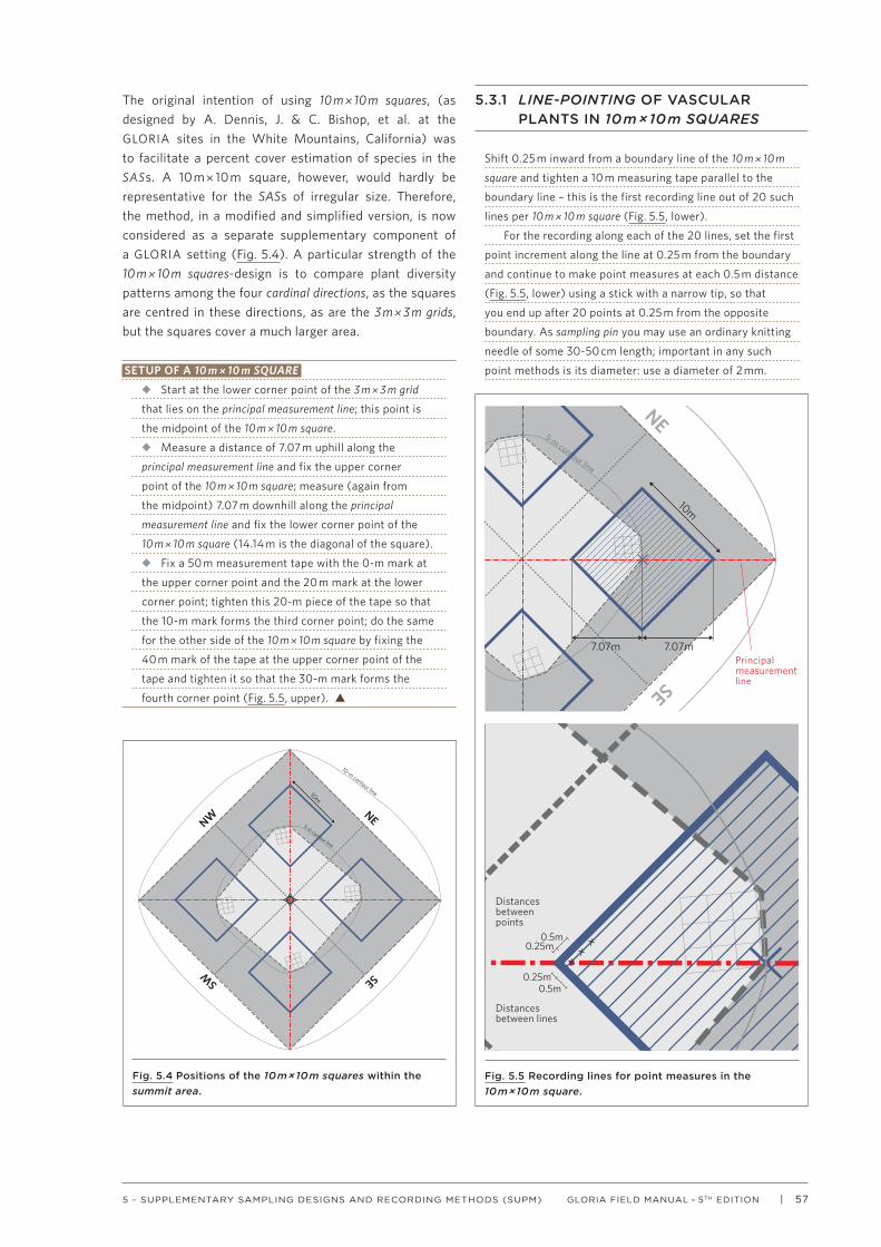
| 57GLORIA FIELD MANUAL – 5TH  EDITION5 - SUPPLEMENTARY SAMPLING DESIGNS AND RECORDING METHODS (SUPM)

The original intention of using 10 m × 10 m squares, (as designed by A. Dennis, J. & C. Bishop, et al. at the GLORIA sites in the White Mountains, California) was to facilitate a percent cover estimation of species in the SASs. A 10 m × 10 m square, however, would hardly be representative for the SASs of irregular size. Therefore, the method, in a modified and simplified version, is now considered as a separate supplementary component of a GLORIA setting (Fig.  5.4). A particular strength of the 10 m × 10 m squares-design is to compare plant diversity patterns among the four cardinal directions, as the squares are centred in these directions, as are the 3 m × 3 m grids, but the squares cover a much larger area.

 SETUP OF A 10  m × 10  m SQUARE 

u Start at the lower corner point of the 3 m × 3 m grid

that lies on the principal measurement line; this point is

the midpoint of the 10 m × 10 m square.

u Measure a distance of 7.07 m uphill along the

principal measurement line and fix the upper corner

point of the 10 m × 10 m square; measure (again from

the midpoint) 7.07 m downhill along the principal

measurement line and fix the lower corner point of the

10 m × 10 m square (14.14 m is the diagonal of the square).

u Fix a 50 m measurement tape with the 0-m mark at

the upper corner point and the 20 m mark at the lower

corner point; tighten this 20-m piece of the tape so that

the 10-m mark forms the third corner point; do the same

for the other side of the 10 m × 10 m square by fixing the

40 m mark of the tape at the upper corner point of the

tape and tighten it so that the 30-m mark forms the

fourth corner point (Fig. 5.5, upper). s

5.3.1 LINE-POINTING OF VASCULAR PLANTS IN 10  m × 10  m SQUARES

Shift 0.25 m inward from a boundary line of the 10 m × 10 m

square and tighten a 10 m measuring tape parallel to the

boundary line – this is the first recording line out of 20 such

lines per 10 m × 10 m square (Fig. 5.5, lower).

For the recording along each of the 20 lines, set the first

point increment along the line at 0.25 m from the boundary

and continue to make point measures at each 0.5 m distance

(Fig. 5.5, lower) using a stick with a narrow tip, so that

you end up after 20 points at 0.25 m from the opposite

boundary. As sampling pin you may use an ordinary knitting

needle of some 30-50 cm length; important in any such

point methods is its diameter: use a diameter of 2 mm.

Fig. 5.4 Positions of the 10 m × 10 m squares within the summit area.

10-m contour line

5-m contour line

NW NE

SESW

10m

Fig. 5.5 Recording lines for point measures in the 10 m × 10 m square.

Distances between lines

0.25m0.5m

Distancesbetweenpoints

0.25m0.5m

5-m contour line

NE

SEPrincipal measurement line

10m

7.07m 7.07m

58 | GLORIA FIELD MANUAL – 5TH  EDITION5 - SUPPLEMENTARY SAMPLING DESIGNS AND RECORDING METHODS (SUPM)

At each point note the species or the surface type you hit

(for details see below).

After having finished recording along this line, shift the

tape by 0.5 m further inward, and so forth; in total recording

is to be made along 20 such lines.

Finally you end up with 400 point measures being

regularly distributed over the 10 m × 10 m square. s

 HOW TO DO THE RECORDING AT EACH POINT 

Hold the sampling pin (or stick) at its top so that you hit the

point perpendicularly to the ground. Note what is hit by the

needle by making a stroke into the relevant cell on the data

sheet. This can either be one of the surface types already

listed on the datasheet (Form 6-S, Annex II) or a vascular

plant species. When hitting a surface type without vascular

plants, make a stroke at one of the listed surface types (only

one stroke per point is possible in this case). When hitting

a vascular plant, write the species name and make a stroke

in the respective recording line. In some cases the needle

may touch more than one species, e.g. when having several

vegetation layers. Make strokes for each species you hit.

Thus, you may end up with more than 20 strokes per line

and more than 400 strokes out of your 400 points per

square. But do not record any of the surface types that lie

below a vascular plant.

Note: that one cell on the sheet can have a maximum of

20 strokes, e.g. if all points on a line fall on solid rock or if

the same species is encountered on all points.

As we are primarily interested in species cover, it makes

sense to record all species you hit with the needle (and not

only the taller growing top-most ones). Even when having

more than 400 strokes, you can still calculate (later on) a

percent cover value for each species hit in the 10 m × 10 m

square: percent species cover = strokes per species/4. Or:

total top cover of vascular plants = (400 minus the sum of

strokes of surface types)/4.

u Starting points and procedure: In principle, you

can start with the first line from any of the four corners

in either of the two possible directions. It is more

comfortable, however, to work uphill; therefore only four

options remain, which are illustrated on Form 6-S (see

Annex II). For resurveys it is advisable to repeat the

procedure in the same way. Therefore, make a check mark

on Form 6-S (upper right corner) at one of the four options.

Record along the 20 lines in the following manner:

On the first line start in the direction as indicated on the

marked sketch, and begin the next line from the opposite

end of the square, and so forth.

u Possible implications: In steep and rugged terrain it

may be difficult to setup the 10 m × 10 m square or to apply

the line- pointing. When terrain is unsuitable because

of steepness, we recommend to skip this method. If a

10 m × 10 m square could, nevertheless, be spread over a

rugged terrain, the square may be distorted and, thus,

recording lines may not properly fit within the boundaries.

Irrespectively of this, always make 20 points per line, start

at 0.25 m from the square boundary and continue at 0.5 m

intervals.

The 10 m × 10 m square stretches over the 3 m × 3 m grid

area, where trampling within the four corner-quadrats

must be strictly avoided. Therefore, leave the 3 m × 3 m grid

mounted to keep this area visible when doing the line-

pointing.

There are some implications when you also record

bryophytes and lichens on the species level (optional):

when you hit a bryophyte or a lichen, make a stroke at

the respective species, but also a stroke at the respective

surface type (either ‘lichens on soil’ or ‘bryophytes on soil’); if

you hit the cryptogam species at a point where you also hit

a vascular plant, do not make an extra stroke at the surface

type. s

5.3.2 RECORDING OF ADDITIONAL SPECIES IN 10  m × 10  m SQUARES

Once you have completed the line-pointing, make a list

of vascular plant species which were not captured by the

pointing. Before doing this, add all additional vascular plant

species which were found in the four 1-m² quadrats – so

keep in mind to do the quadrat recording first. All additional

species in the 100-m² area, on average, do not cover more

than 0.25%. Their capture, however, is of relevance for

comparing species richness at different nested spatial levels

(1-m², 4-m², 100-m², and the larger area of the combined

upper and lower SAS).

The basic recording in the 10 m × 10 m squares only

involves line-pointing and an inventory (list of species) of

all vascular plant taxa which were not hit by line-pointing,

but not their visual cover estimation. More detailed species

inventories in 1 m × 10 m bands can be made supplementally,

especially when doing the Downslope Plant Survey. For

details see the note on additional sampling in 10 m × 10 m

squares in chapter 7.1. s

For the sampling sheet see Form 6-S in Annex II.

| 59GLORIA FIELD MANUAL – 5TH  EDITION6 - DATA HANDLING AND MANAGEMENT

6.1 THE SPECIES LIST

The first step of the data entry procedure is the preparation of a complete list of all (vascular plant) taxa found on the four summit sites of a GLORIA target region.

Use the GLORIA “Taxa input sheet (xls)” for entering all your species data. Table 6.1 explains the fields to be filled out for each taxon. The Taxa input sheet can be downloaded from the GLORIA website (www.gloria.ac.at) and an example is appended in Annex II, Part 2.

Carefully check your sampling sheets in order to capture all taxa that were recorded on the summit sites. This includes both the sampling sheets of the summit area sections as well as of the 1-m² quadrats. Make sure that all taxa are properly identified. Make one single list that contains all taxa found on the four summit sites of your GLORIA target region. While entering your taxa, also check the over-all GLORIA species list at www.gloria.ac.at for already listed “accepted” names and synonyms. Where applicable, use the names listed in the over-all GLORIA species list even though they might be outdated.

Doubtful and incomplete identifications:Cases where the identification remained doubtful should be treated in the same way as the clearly identified taxa in the species list. In such cases, however, do not forget to tick “cf.” (confer) later on when you do the actual data input by using the GLORIA data input tools.

For taxa which could not be identified down to the species level, see the example sheet Taxa input sheet example (Annex II, Part 2) on how to enter such cases. Both unidentified species and species where identification is doubtful require at least one herbarium specimen (but not collected within the permanent plots).

Send the completed Taxa input sheet to the GLORIA coordination (office@gloria.ac.at). The file should be renamed as: CC_TTT_GLORIA_TAXA_INPUT_YYYYMMDD.xls with CC country code, TTT target region code, YYYYMMDD current date (year month day).

The GLORIA coordination will check all taxa names for consistency and synonymy in order to achieve an unambiguous GLORIA-wide list, which usually requires consultation with the field team. All fields will be checked for completeness and consistency so that data can be entered into the central GLORIA database (CGDB). Please be very careful when preparing your taxa list, i.e. strictly stay with the formats shown in the example sheet “Taxa input sheet EXAMPLE (xls)” and clean up your file from any special formats, hyperlinks, etc. Add the target region code and the contact person on the excel sheet.

6 DATA HANDLING AND MANAGEMENT

Table 6.1  The GLORIA taxa input sheet (see an example in Annex II)

FIELD FIELD DESCRIPTION

FULL_NAME Full taxon name including the taxon author(s) or his/her/their abbreviation(s)

PLANT_TYPE V = vascular plant, B = bryophyte, L = lichen

RANK Taxonomic rank; possible standard entries: “species”, “subsp.” (subspecies), “var.” (variety); in cases where the species cannot be identified, use: “agg.” (aggregate species), “genus”, or “family”

FLORA Abbreviation of the flora (literature) used; in addition give the full citation of the flora. Where ever possible, please use floras with a large geographical coverage, preferably with checklists accessible in the internet

FAMILY Plant family

GENUS Genus name

SPECIES Species name (epithet)

TAXON If RANK is “species” or “agg.”, enter again the name of the species (or of the aggregate species); if RANK is a lower taxonomic level, enter the name of the subsp. or var. In all cases higher than species (genus, family etc.) enter the full Target Region code (e.g. ATHSW)

REFERENCE The nomenclatural reference; i.e. the reference of the first publication of the name.

SYNONYMS Where applicable, add synonymous names of the taxon, particularly when widely used ones exist (including the taxon author (s) or abbreviation(s) - if more than one synonym, divide by a semicolon (;)

SPECIES_No_in_FLORA The code number (numerical or alphanumerical) which is used in the flora reference which you entered in the column “FLORA”, (where applicable)

B_LIVERWORT Only relevant for bryophytes: enter “true” if the bryophyte is a liverwort, “false” if it is a moss

COMMENT Text field for comments; e.g. on taxonomical details in the case of a critical taxon

HERBARIUM_SPECIMEN Enter the code of your herbarium voucher: Herbarium acronym, collector, voucher number (this is obligatory for doubtful cases) - further, indicate the name of the herbarium and its location (on the herbarium voucher write the summit code)

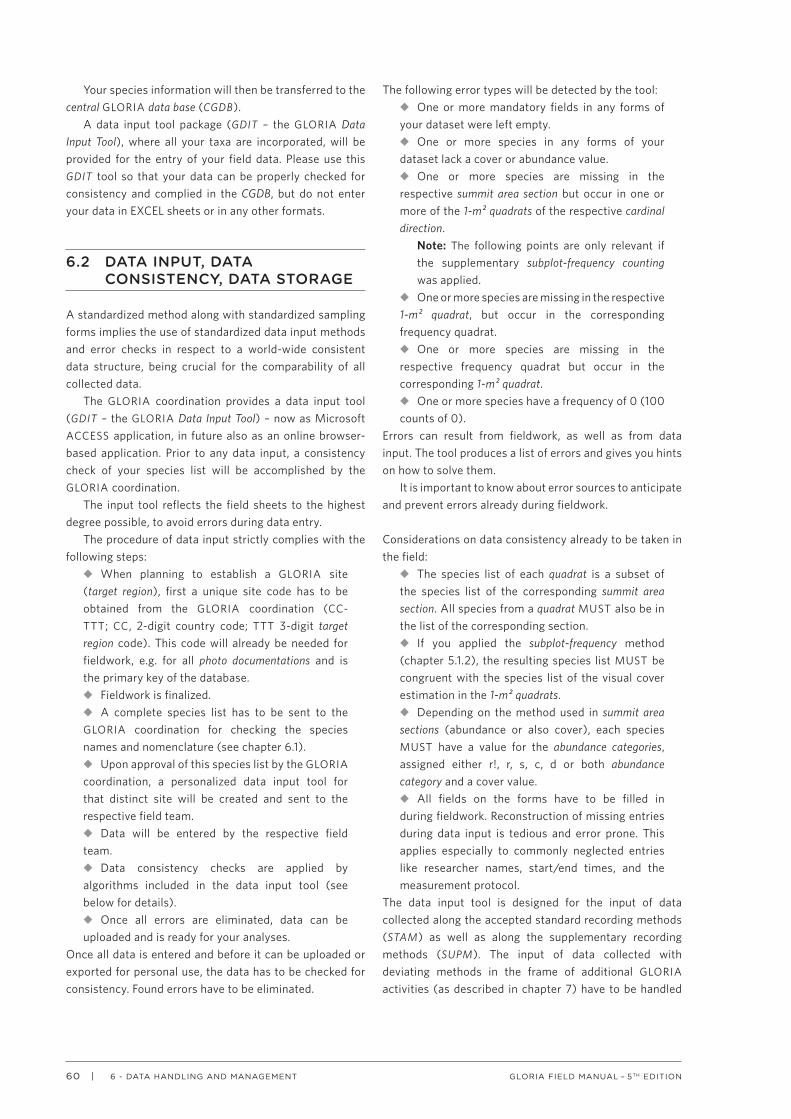
60 | GLORIA FIELD MANUAL – 5TH  EDITION6 - DATA HANDLING AND MANAGEMENT

Your species information will then be transferred to the central GLORIA data base (CGDB).

A data input tool package (GDIT – the GLORIA Data Input Tool), where all your taxa are incorporated, will be provided for the entry of your field data. Please use this GDIT tool so that your data can be properly checked for consistency and complied in the CGDB, but do not enter your data in EXCEL sheets or in any other formats.

6.2 DATA INPUT, DATA CONSISTENCY, DATA STORAGE

A standardized method along with standardized sampling forms implies the use of standardized data input methods and error checks in respect to a world-wide consistent data structure, being crucial for the comparability of all collected data.

The GLORIA coordination provides a data input tool (GDIT – the GLORIA Data Input Tool) – now as Microsoft ACCESS application, in future also as an online browser-based application. Prior to any data input, a consistency check of your species list will be accomplished by the GLORIA coordination.

The input tool reflects the field sheets to the highest degree possible, to avoid errors during data entry.

The procedure of data input strictly complies with the following steps:

u When planning to establish a GLORIA site (target region), first a unique site code has to be obtained from the GLORIA coordination (CC-TTT; CC, 2-digit country code; TTT 3-digit target region code). This code will already be needed for fieldwork, e.g. for all photo documentations and is the primary key of the database.u Fieldwork is finalized.u A complete species list has to be sent to the GLORIA coordination for checking the species names and nomenclature (see chapter 6.1).u Upon approval of this species list by the GLORIA coordination, a personalized data input tool for that distinct site will be created and sent to the respective field team.u Data will be entered by the respective field team.u Data consistency checks are applied by algorithms included in the data input tool (see below for details).u Once all errors are eliminated, data can be uploaded and is ready for your analyses.

Once all data is entered and before it can be uploaded or exported for personal use, the data has to be checked for consistency. Found errors have to be eliminated.

The following error types will be detected by the tool: u One or more mandatory fields in any forms of your dataset were left empty.u One or more species in any forms of your dataset lack a cover or abundance value.u One or more species are missing in the respective summit area section but occur in one or more of the 1-m² quadrats of the respective cardinal direction.

Note: The following points are only relevant if the supplementary subplot-frequency counting was applied.

u One or more species are missing in the respective 1-m² quadrat, but occur in the corresponding frequency quadrat. u One or more species are missing in the respective frequency quadrat but occur in the corresponding 1-m² quadrat.u One or more species have a frequency of 0 (100 counts of 0).

Errors can result from fieldwork, as well as from data input. The tool produces a list of errors and gives you hints on how to solve them.

It is important to know about error sources to anticipate and prevent errors already during fieldwork.

Considerations on data consistency already to be taken in the field:

u The species list of each quadrat is a subset of the species list of the corresponding summit area section. All species from a quadrat MUST also be in the list of the corresponding section.u If you applied the subplot-frequency method (chapter 5.1.2), the resulting species list MUST be congruent with the species list of the visual cover estimation in the 1-m² quadrats.u Depending on the method used in summit area sections (abundance or also cover), each species MUST have a value for the abundance categories, assigned either r!, r, s, c, d or both abundance category and a cover value.u All fields on the forms have to be filled in during fieldwork. Reconstruction of missing entries during data input is tedious and error prone. This applies especially to commonly neglected entries like researcher names, start/end times, and the measurement protocol.

The data input tool is designed for the input of data collected along the accepted standard recording methods (STAM) as well as along the supplementary recording methods (SUPM). The input of data collected with deviating methods in the frame of additional GLORIA activities (as described in chapter 7) have to be handled

| 61GLORIA FIELD MANUAL – 5TH  EDITION6 - DATA HANDLING AND MANAGEMENT

by the particular target region team or by the coordinating group of a particular additional activity. A central data storage at the GLORIA coordination, however, is planned to be offered for additional activities.

The GLORIA coordination maintains the central GLORIA Database (CGDB) to the state of the art of data storage standards. Apart from that, each site team has to take care of their data storage by their own. In addition, archive your original and scanned field sheets.

Over the longer term, personal turnover in groups will occur and some target regions may get orphaned. Notwithstanding this, the value of permanent plots and data will increase by years, as long as the full datasets (including the necessary photos for plot reassignment) are properly stored and accessible for future generations of researchers. Besides the double storage of data in the central CGDB as well as at each team’s institution, publishing of the complete target region data would be a worthwhile effort.

6.3 HANDLING OF THE PHOTO DOCUMENTATION

The original photo documentation materials should be stored in your office* together with your original field forms for further monitoring. But photos must as well be delivered digitally with standardised file names (see Box 6.1) to the GLORIA coordination so that they can be directly included in the central GLORIA Database (CGDB).

*Past experience has shown that depositing photos and other documentation in institution libraries may be a more robust archiving strategy as staff leave, where records may be lost.

Use the high-resolution images as you have taken in the field. All digital photo files have to be renamed according to the GLORIA-unique coding system. Please see Box  6.1 and Annex III as well as the GLORIA web site for more information on how to do this and to deliver the materials to the GLORIA coordination.

Various items in the GLORIA dataset must have a GLORIA-wide specific coding, which is used in forms, on photographs, for temperature loggers, as well as in the database.

u Country codes: The two-digit ISO 3166 codes are used. Examples: AT for Austria, CA for Canada, CL for Chile, GE for Georgia, NZ for New Zealand, RU for Russia.u Target region codes: These three-digit alphanumeric codes are created solely by the GLORIA coordi-nation to avoid code conflicts; please contact us to obtain a target region code. Examples: SNE is Sierra Neva-da/Spain, GNP is Glacier National Park, Montana/USA, MJW is Ma-Ji-Wa, Hengduan Shan, Yunnan/China.u Summit codes: Three-digit char-acter codes (avoid numbers). Each researcher who is responsible for a target region shall select such codes for his/her summits, avoiding coding conflicts within the TR. Examples: BAR is Mount Barcroft, GHK is Ghacktkogel, MPO is Maly Pourkeu, PFO is Piz Foraz.

››  These three code elements must be indicated in the header of any field protocol form.

u All measurement points. Their codes are indicated in Fig. 3.2.u All sampling areas. Their codes are indicated in Fig. 3.2. Special care

should be devoted to the coding of 1-m² quadrats, as indicated in Fig. 4.1. For example, if you stand below the lower boundary of a southern 3 m × 3 m quadrat cluster, and look towards the summit, then the left lower 1-m² quad-rat is coded S11 (the first column and first row of the cluster), whereas the right lower quadrat is coded S31 (the third column and first row). The other quadrats are coded in a similar way according to their column-row-posi-tion in the cluster, S13, S33, and S22 for the middle quadrat where loggers are positioned. This coding is similar to what is used in many geographic maps and GIS applications.u Full-length-codes: These are used for items that may be used or recorded separately from sampling protocols Forms 0, 1−4, 5-S, 6-S. Such items should be coded with full-length-codes, which are a combi-nation of the country-, target region-, and summit-code followed by other specific code elements.

They are used, e.g. for:u Temperature data loggers: For each logger, indicate the logger posi-tion and installation year on the log-ger and in the protocol as:

CC_TTT_SSS_QQQ_YYYY with CC: countrycode, TTT: target region code, SSS: summit code, QQQ: quad-rat code (see Fig. 4.1), YYYY: (year) of installation of the logger in the field.

Example for logger position and installation year:

v ES_SNE_TCA_W22_2002 for a temperature logger in Spain, Sierra Nevada, Pico del Tosal Cartujo, western 3 m × 3 m quadrat cluster - quadrat 22, installed in 2002.u Photographs: A blackboard with indications must be included in the photo view (see chapter 4.4). Whenever a distinct GLORIA item is photographed, such as measurement points, plots, temperature data loggers, indicate the relevant code elements in the correct sequence. As separator of the code elements you may use a point (.) to save space on the black-board.

On any photo, do not forget to indicate the date on the blackboard in the sequence YYYY-MM-DD.

Examples for photo codes are:v AT_HSW_GHK_N33__20010817 for a photograph of a 1-m² quadrat in Austria, Hochschwab, Ghack-tkogel, 1-m² quadrat N33, on 17th August 2001.v ES_SNE_TCA_p10m-S__20080703 for a photograph of: Spain, Sierra Nevada, Pico del Tosal Cartujo, southern summit area corner point at the 10-m level, on 3rd July 2008.

On photos of data loggers, also write the prefix LOG- in front of the plot code onto the blackboard (e.g. ES_SNE_TCA_LOG-W22).

BOX 6.1 GLORIA-UNIQUE CODES FOR VARIOUS ITEMS IN FORMS AND PHOTOGRAPHS

62 | GLORIA FIELD MANUAL – 5TH  EDITION6 - DATA HANDLING AND MANAGEMENT

6.4 DATA PROPERTY RIGHTS AND DATA SHARING

For all data which are included in the central GLORIA Database (CGDB; such as on species, habitat and site properties, soil temperature, and photo data) the following rules apply:

u Every contributor of field data retains the exclusive ownership of the data.u Only persons and teams who have contributed data to the central GLORIA Database are eligible to be part of data sharing. This, however, should not restrict cooperation between GLORIA members (data providers) and external persons for analysis and publication of their GLORIA data.u The use of a site dataset or of parts of it by eligible members of the GLORIA network requires the data provider’s permission.u The authorship of intended publications must be negotiated between the data requester and the data owner(s).

These rules require the following procedure:u Eligible data requesters, who wish to use data from other sites, must submit a request to the GLORIA coordination (office@gloria.ac.at), which contains:

v A description of the intended data analysis including hypothesis, methods and expected results.v A detailed description which data are needed: sites (target regions), monitoring cycle(s), plot types, habitat and site properties, soil temperature, photo data, species presence/absence, species cover, species subplot-frequency, or on particular species groups.v A suggestion for lead and co-authorships.

u The GLORIA coordination will discuss the proposal (i) regarding other planned activities in the GLORIA consortium; (ii) with the requester; and (iii) with the data owners.u Upon consent, the GLORIA coordination will send the negotiated dataset to the requester.u The data requester guarantees that the data are only used for the negotiated purpose.

Any further analysis on this dataset requires a new request.

Re-use, redistribution and the production of derivates are usually based on published data and therefore underlie the policies of the respective journal or publisher. The re-use of unpublished material requires permission of the data provider.

Selection of sites and data sets for data analysis: For analyses of GLORIA data including large-scale analyses, no specific regulation or selection criteria on which sites or data sets are included can be given. This of course depends on the respective research question and the completeness of required data sets, which e.g. may focus on selected biomes, on particular bedrock types, on sites with at least one or with multiple resurvey data sets or even on sites with data sets from a particular time period.

| 63GLORIA FIELD MANUAL – 5TH  EDITION7 - EXTRA APPROACHES IN GLORIA (EXAP)

This chapter shows that the GLORIA programme has grown well beyond its standard Multi-Summit Approach after its first decade of operation. Apart from standard and supplementary methods for GLORIA summit sites, several additional activities have started as further components of the GLORIA network. These extra approaches are directly related to a GLORIA target region, but are usually not confined to the summit sites, and partly have an interdisciplinary focus. This chapter describes an array of further monitoring and data collection activities which are directly related to GLORIA target regions. These activities focus either on extended spatial designs and/or on topics other than summit vegetation, such as on other organism groups, ecosystem components or on socio-economic and cultural aspects. They were already presented at the international GLORIA conference, held in Perth, Scotland, in September 2010. All approaches have been initiated, developed and applied in the field by various GLORIA teams on different continents.

The first subchapter 7.1 deals with plant species monitoring along downslope belt transects of GLORIA summits to the upper forest belt. Its principal target is to identify the regional lower and upper range limits of species distributions.

The following three subchapters focus on various animal organism groups in different sampling approaches in GLORIA target regions: 7.2 on pitfall trapping of invertebrates, 7.3 on other methods of invertebrate sampling and 7.4 on herpetological monitoring around and downslope from the GLORIA summit sites. Further we refer here to a recent comprehensive account on faunistic (mostly arthropod) monitoring at GLORIA summit habitats in the Alps (ÖKOTEAM 2014).

Subchapter 7.5 contains approaches to survey the soil variability around GLORIA summit sites. The final two subchapters deal with socio-economic and cultural aspects in GLORIA target regions. In 7.6 the recognition of past and current anthropogenic factors concerning land use practices and socio-economic implications are attempted. Chapter 7.7 focuses on ethnobotany in the context of local people’s perception of adaptations to and mitigations of climate change.

Descriptions of these thematic subchapters differ in the level of development and standardisation. Further method elaboration and testing and subsequent step-by-step descriptions of working procedures are still required for some of these extra approaches.

On the other hand, further GLORIA-related activities were recently emerging in the following fields, which should be mentioned here in brief:

Focus on plant functional traits (PFTs): This can considerably build on extensive previous research (e.g. Halloy & Mark 1996, Cornelissen et al. 2003, Pohl et al. 2011, Venn et al. 2011) and is to a large part a matter of collateral data which may be obtained from existing literature and data bases (see, e.g., Cornelissen et al. 2003, Landolt et al. 2010). The identification and use of suitable plant functional traits holds an outstanding potential for GLORIA in comparing vegetation of different biomes with little or no floristically overlapping species composition. Especially, this information may prove useful in developing predictive models of responses of plants with particular traits to changes in abiotic factors, and in the overall view, to climate change. Researchers within the GLORIA programme are in the process of collecting field, lab, and collated data on plant functional traits of the species at their respective GLORIA sites, such as initiated through an INTERACT project at the Cairngorms GLORIA site, Scotland, and a recent North American/European collaboration (contact Martha Apple, Montana Tech) or have compared functional leaf traits with summit species data at the Snowy Mountains GLORIA site, Australia (Venn et al. 2014).

Focus on experimental warming: Experimental studies using open-top-chambers (Molau & Mølgaard 1996) and eco-physiological measurements were recently started at tropical and subtropical GLORIA sites in Ecuador and N-Argentina. These new experimental sites, being of course established well outside of the GLORIA summit sites, would provide valuable links and possibilities of comparison with long-established networks such as the International Tundra Project (ITEX, http://www.geog.ubc.ca/itex/). Contact: Francisco Cuesta, Priscilla Muriel, CONDESAN, Catholic University Quito, respectively.

Focus on ecosystem services: An assessment of ecosystem services in GLORIA target regions / catchment areas, using a new rapid assessment method developed for the LTER-Europe network (Dick et al. 2014) may be applied in a wider GLORIA context and could also contribute to the further development of GLORIA activities described in the subchapters 7.6 and 7.7. Contact: Jan Dick, CEH Scotland.

The key responsibilities for the further elaboration, wider application and supervision of any of the extra approaches and activities mentioned and described in this chapter lie with the particular expert groups. Their status and progress, however, is planned to be also displayed on the GLORIA website including eventual future activities which are not yet mentioned in this manual.

7 EXTRA APPROACHES IN GLORIA (EXAP)

64 | GLORIA FIELD MANUAL – 5TH  EDITION7 - EXTRA APPROACHES IN GLORIA (EXAP)

REFERENCES (CHAPTER 7, INTRODUCTION)

Cornelissen, J. H. C.; Lavorel, S.; Garnier, E.; Diaz, S.; Buchmann, N.; Gurvich, D. E.; Reich, P. B.; ter Steege, H.; Morgan, H. D.; van der Heijden, M. G. A.; Pausas, J. G. & Poorter, H. (2003). A handbook of protocols for standardised and easy measurement of plant functional traits worldwide. Australian Journal of Botany 51: 335–380.

Dick, J.; Al-Assaf, A.; Andrews, C.; Díaz-Delgado, R.; Groner, E.; Halada, L.; Izakovicova, Z.; Kertész, M.; Khoury, F.; Krašić, D.; Krauze, K.; Matteucci, G.; Melecis, V.; Mirtl, M.; Orenstein, D. E.; Preda, E.; Santos-Reis, M.; Smith, R. I.; Vadineanu, A.; Veselić, S. & Vihervaara, P. (2014). Ecosystem services: a rapid assessment method tested at 35 sites of the LTER-Europe network. Ekologia 33: 217-231.

Halloy, S. R. P. & Mark, A. F. (1996). Comparative leaf morphology spectra of plant communities in New Zealand, the Andes and the European Alps. Journal of the Royal Society of New Zealand 26: 41–78.

Landolt, E.; Bäumler, B.; Erhardt, A.; Hegg, O.; Klötzli, F.; Lämmler, W.; Nobis, M.; Rudmann-Maurer, K.; Schweingruber, F. H.; Theurillat, J.-P.; Urmi, E.; Vust, M. & Wohlgemuth, T. (2010). Flora indicativa: Ökologische Zeigerwerte und biologische Kennzeichen zur Flora der Schweiz und der Alpen / Ecological indicator values and biological attributes of the Flora of Switzerland and the Alps. Haupt Verlag, Bern.

Molau, U. & Mølgaard, P. (1996). International Tundra Experiment, ITEX Manual, second edition. Danish Polar Center, Copenhagen.

Ökoteam (2014). Gipfelfauna-Monitoring im Nationalpark Gesäuse. Monitoring der Gipfelfauna unter besonderer Berücksichtigung sensibler, gefährdeter und endemischer Spinnentier- und Insektentaxa. Unveröffentlichter Projektbericht im Auftrag der Nationalpark Gesäuse GmbH.

Pohl, M.; Stroude, R.; Buttler, A. & Rixen, C. (2011). Functional traits and root morphology of alpine plants. Annals of Botany 108: 537–545.

Venn, S.; Pickering, C. & Green, K. (2014). Spatial and temporal functional changes in alpine summit vegetation are driven by increases in shrubs and graminoids. AoB plants 6: doi:10.1093/aobpla/plu1008.

Venn, S. E.; Green, K.; Pickering, C. M. & Morgan, J. W. (2011). Using plant functional traits to explain community composition across a strong environmental filter in Australian alpine snowpatches. Plant Ecology 212: 1491–1499.

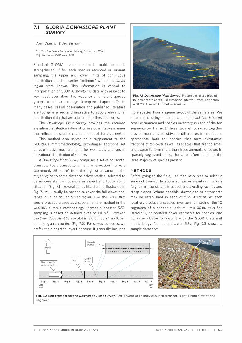
| 65GLORIA FIELD MANUAL – 5TH  EDITION7 - EXTRA APPROACHES IN GLORIA (EXAP)

7.1 GLORIA DOWNSLOPE PLANT SURVEY

Ann Dennis¹ & Jim Bishop²

1 | The CalFlora Database, Albany, California, USA; 2 | Oroville, California, USA

Standard GLORIA summit methods could be much strengthened, if for each species recorded in summit sampling, the upper and lower limits of continuous distribution and the center ‘optimum’ within the target region were known. This information is central to interpretation of GLORIA monitoring data with respect to key hypotheses about the response of different species groups to climate change (compare chapter 1.2). In many cases, casual observation and published literature are too generalized and imprecise to supply elevational distribution data that are adequate for these purposes.

The Downslope Plant Survey provides the required elevation distribution information in a quantitative manner that reflects the specific characteristics of the target region.

This method also serves as a supplement to the GLORIA summit methodology, providing an additional set of quantitative measurements for monitoring changes in elevational distribution of species.

A Downslope Plant Survey comprises a set of horizontal transects (belt transects) at regular elevation intervals (commonly 25-metre) from the highest elevation in the target region to some distance below treeline, selected to be as consistent as possible in aspect and topographic situation (Fig. 7.1). Several series like the one illustrated in Fig. 7.1 will usually be needed to cover the full elevational range of a particular target region. Like the 10 m × 10 m square procedure used as a supplementary method in the GLORIA summit methodology (compare chapter 5.3), sampling is based on defined plots of 100 m². However, the Downslope Plant Survey plot is laid out as a 1 m × 100 m belt along a contour line (Fig. 7.2). For survey purposes, we prefer the elongated layout because it generally includes

more species than a square layout of the same area. We recommend using a combination of point-line intercept cover estimation and species inventory in each of the ten segments per transect. These two methods used together provide measures sensitive to differences in abundance appropriate both for species that form substantial fractions of top cover as well as species that are too small and sparse to form more than trace amounts of cover. In sparsely vegetated areas, the latter often comprise the large majority of species present.

METHODSBefore going to the field, use map resources to select a series of transect locations at regular elevation intervals (e.g. 25 m), consistent in aspect and avoiding ravines and steep slopes. Where possible, downslope belt transects may be established in each cardinal direction. At each location, produce a species inventory for each of the 10 segments of a horizontal belt of 1 m × 100 m, point-line intercept (line-pointing) cover estimates for species, and top cover classes consistent with the GLORIA summit methodology (compare chapter 5.3). Fig.  7.3 shows a sample datasheet.

Fig. 7.1 Downslope Plant Survey. Placement of a series of belt transects at regular elevation intervals from just below a GLORIA summit to below treeline.

Leftend

Rightend

Photo view for one segment

Samplepoints

Tape Origin point

Seg. 1 Seg. 2 Seg. 3 Seg. 4 Seg. 5 Seg. 6 Seg. 7 Seg. 8 Seg. 9 Seg. 10

Uphill

Cover = #hits;400 total

Cover = #hits;400 total

Frequency = #segments;10 total

Frequency = #segments;10 total

Fig. 7.2 Belt transect for the Downslope Plant Survey. Left: Layout of an individual belt transect. Right: Photo view of one segment.

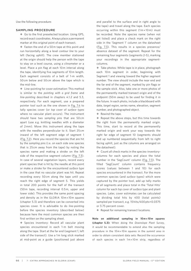
66 | GLORIA FIELD MANUAL – 5TH  EDITION7 - EXTRA APPROACHES IN GLORIA (EXAP)

Use the following procedure:

SAMPLING PROCEDUREu Go to the first preselected location. Using GPS, record exact coordinates. Always place a permanent marker at this original point of each transect.u Fasten the end of a 50 m tape at this point and run horizontally along a level contour line to your left (facing uphill). The crew member stationed at the origin should help the person with the tape to stay on a level course, using a clinometer or a level. Place a pin flag at each 10 m interval along the tape, identifying five segments of 10 m length. Each segment consists of a belt of 1-m width, 50 cm below and 50 cm above the tape which is the mid-line.u Line-pointing for cover estimation: This method is similar to the pointing with a grid frame and line-pointing described in chapters 4.1.2 and 5.3, respectively. For each segment, use a prepared pointer tool such as the one shown in Fig.  7.4 to tally species cover (or top cover of surface types where no vascular plant occurs). The instrument should have two sampling pins that are 50 cm apart (use e.g. knitting needles with a diameter of 2 mm). Move this instrument along the tape with the needles perpendicular to it. Start 25 cm inward of the left segment edge of segment 1 (Fig. 7.2). Here you record the species that are hit by the sampling pins (i.e. on each side one species that is 25 cm away from the tape) by noting the species name and making a stroke on the left side of the respective segment column (Fig.  7.3). In case of several vegetation layers, record every plant species that is hit by the needle at this point or make a stroke for the encountered surface type in the case that no vascular plant was hit. Repeat recording every 50 cm along the tape until you reach the right edge of segment 5. This yields in total 200 points for the half of the transect (50 m tape, recording interval 0.5 m, upper and lower side). This provides the same point spacing and density as in the GLORIA 10 m × 10 m squares (chapter 5.3) and therefore can be converted into species cover. It is advisable to do line-pointing before the species inventory (described below) because here the most common species are then first written on the sampling sheet.u Species inventory: Record all vascular plant species encountered in each 1-m belt moving along the tape. Start at the far end (segment 1, left side of the transect). Use a 1 m long stick marked at mid-point as a guide (positioned just above

and parallel to the surface and in right angle to the tape) and travel along the tape. Each species occurring within this segment (1 m × 10 m) must be recorded. Note the species name (when not yet listed) and place a check mark on the right side in the ‘Segment 1’ column on the datasheet (Fig.  7.3). This results in a species presence/absence dataset of the segment. Repeat for the remaining four segments (segments 2-5), marking your recordings in the appropriate segment-columns.u Take photos: While tape is in place, photograph each 10 m segment in order, beginning with Segment 1 and viewing toward the higher segment number. The view should include the near end and the far end of the segment, marked by pin flags or the sample stick. Also, take one or more photos of the permanently marked transect origin and of the endpoint (50 m away) to be used for finding it in the future. In each photo, include a blackboard with date, target region, series name, elevation, segment number, and photographed object.u Rewind the tape.u Repeat the above steps, but this time towards the right from the permanently marked origin. This time, start to record at the permanently marked origin and work your way towards the right far edge of segment 10 (segments should end up numbered sequentially from left to right facing uphill, just as the columns are arranged on the datasheet).u Count all check marks in the species-inventory-columns for each species and place the total number in the ‘SegCount’ column (Fig.  7.3). The filled ‘SegCount’ column contains frequency scores (values between 1 and 10) for each species encountered in the transect. For the more common species (and surface types) which were captured by the pointer tool, add up tally marks of all segments and place total in the ‘Total Hits’ column for each top cover of surface type and plant species. Later, cover estimates can be calculated by dividing total hits by 400 (total points) sampled per transect, e.g. 15 hits/400 pts=0.0375 or 3.75 percent cover.u Repeat for remaining transect locations.

Note on additional sampling in 10  m × 10  m squares (chapter  5.3): When doing the Downslope Plant Survey, it would be recommendable to extend also the sampling procedure in the 10 m × 10 m squares in the summit area in order to obtain consistent data sets: Record the occurrence of each species in each 1 m × 10 m strip, regardless of

| 67GLORIA FIELD MANUAL – 5TH  EDITION7 - EXTRA APPROACHES IN GLORIA (EXAP)

D OW N S LO P E P L A N T S U RV E Y

Country Target Region Series Name Transect # Latitude Longitude Aspect Elevation Date Time: from to Observers

Transect segment (from left to right as you face uphill)

1 2 3 4 5 6 7 8 9 10

Cover type Line-pointing hits Total

Bare ground

Litter

Rock

Scree

Total hits for column

Plant species Line-pointing hits | Species inventory Total

| | | | | | | | | | |

| | | | | | | | | | |

| | | | | | | | | | |

| | | | | | | | | | |

| | | | | | | | | | |

| | | | | | | | | | |

| | | | | | | | | | |

| | | | | | | | | | |

| | | | | | | | | | |

| | | | | | | | | | |

| | | | | | | | | | |

| | | | | | | | | | |

| | | | | | | | | | |

| | | | | | | | | | |

| | | | | | | | | | |

| | | | | | | | | | |

| | | | | | | | | | |

| | | | | | | | | | |

| | | | | | | | | | |

| | | | | | | | | | |

| | | | | | | | | | |

| | | | | | | | | | |

| | | | | | | | | | |

| | | | | | | | | | |

| | | | | | | | | | |

| | | | | | | | | | |

| | | | | | | | | | |

| | | | | | | | | | |

| | | | | | | | | | |

| | | | | | | | | | |

| | | | | | | | | | |

| | | | | | | | | | |

| | | | | | | | | | |

| | | | | | | | | | |

| | | | | | | | | | |

Fig. 7.3 Downslope Plant Survey datasheet.

Comments:

68 | GLORIA FIELD MANUAL – 5TH  EDITION7 - EXTRA APPROACHES IN GLORIA (EXAP)

whether it receives a hit or not. That process is referred to as “species inventory”, being exactly analogous to that applied in the Downslope Plant Survey. You can do that by placing the guide string in between each mark used for the point counts (i.e. at the “half-meter” points), and noting the presence of all species in a strip that extends 50 cm on each side of the string.

EQUIPMENTFor each transect team: GPS device and map; datasheets; clipboard and pencil; camera; 50 m tape; 1 m stick marked at mid-point; pointer tool (see Fig.  7.4); blackboard and chalk; 15 pinflags; sticks for permanent marking.

TIMELINESDepending on vegetation, team size, and level of experience, the sampling procedure described above typically takes from 1 to 2.5 hours for a 1 m × 100 m belt transect. More species, challenging identifications, and/or less rock extend the time required. Typical is for a single transect team of 4 people to complete 3 or 4 100-meter transects per field day.

EFFICIENCY HINTSTwo people are the minimum team for carrying out this procedure. Extra personnel are best grouped into additional work pairs. Several two person teams can work simultaneously on different tasks at the same transect location, or teams can work on different transects. Bring additional equipment and datasheets to accommodate multiple teams.

EXAMPLE: A DOWNSLOPE PLANT SURVEY IN THE WHITE MOUNTAINS (CALIFORNIA)The composite survey on 41 1 m × 100 m belt transects spanned over 1000 m of elevation (belt transect locations at 25 m vertical intervals) from 25 m below the highest summit to 300 m below the lowest summit. An example of vegetation top cover and of distribution data for selected species from our Downslope Plant Survey work is shown in Table 7.1 . Point intercept sampling provided percent cover estimates of herbaceous/dwarf shrub vegetation and overstory trees. These document locations of treeline and transitions in vegetation cover

Table 7.1 Example of data from belt transects, White Mountains Downslope Plant Surveys (41 belt transects ranging from 4300 to 3300 m a.s.l.). Percent species cover of vascular plant vegetation (divided into tree and low-stature herbaceous/shrub vegetation) using the point intercept method and frequency scores of selected species are shown. Regionally relevant altitudinal species profiles (AL-AC-AU: AL Altitudinal zones of lower margin, AC center, and AU upper margin of continuous species distribution; see glossary and Gottfried et al. (2012), can be defined by these data. Full names of species: Erigeron vagus Payson, Festuca brachyphylla J.A. Schultes ex J.A. & J.H. Schultes subsp. coloradensis Frederiksen, Phlox condensata (Gray) E. Nels., Potentilla pseudosericea Rydb., Castilleja nana Eastw., Arenaria kingii (S. Wats.) M.E. Jones var. glabrescens (S. Wats.) Maguire, Erigeron clokeyi Cronq. AL-AC-AU species profiles: al alpine, id indifferent, mo montane, ni nival, tl treeline ecotone.

White Mountains Downslope Survey 2007-2008

Nival Upper Alpine Lower Alpine Treeline ecotone Montane

Tree layer percent cover6 26 29 27 15 25

Understorey herbaceous/ shrub percent cover 1 0 0 0 0 2 1 8 1 29 10 26 30 22 17 44 29 36 28 41 32 56 51 24 15 21 35 13 31 24 16 19 17 15 8 5 6 10 6 3 3

elevation (m) 4300 4200 4100 4000 3900 3800 3700 3600 3500 3400 3300

Altitudinal distribution AL AC AU

ERIG VAGU ni ni ni 4 6 6 7 10 9 9 7 6

FEST BRAC al id ni 4 8 7 5 3 5 3 6 2 2 7 7 3 8 7 5 8 5 2 3 1 3

PHLO COND mo id al 4 2 7 5 8 10 7 7 4 5 10 4 10 9 9 10 10 10 10 9 9 10 10 9 9 8 5 9 8 5

POTE PSEU al al ni 2 2 5 1 1 1 2 2 2 1 2

CAST NANA mo al/tl ni 2 1 1 2 1 1 2 2 2 6 5 6 9 8 9 5 8 5 3 10 6 3 1 1 1

AREN KING mo tl al 2 2 4 7 10 7 8 10 9 10 10 9 10 10 9 10 7 9 10 10 10

ERIG CLOK mo id tl 8 10 9 8 9 9 9 9

Fig. 7.4 A pointer tool with two sampling pins for sampling a pair of points 0.5 m apart.

| 69GLORIA FIELD MANUAL – 5TH  EDITION7 - EXTRA APPROACHES IN GLORIA (EXAP)

at the treeline ecotone and the alpine-nival ecotone. Frequency scores (number of segments out of 10) provide a basis for interpretations of lower and upper margins and center (optimum) zone (cf. Gottfried et al. 2012) for all individual species, most of which are too sparse to show up in point intercept sampling. The example in Table 7.1 only shows a subset of species representing the different types of elevational distribution ranges. The example data reflect the previously used 100-point methodology, which has been updated to the 400-point method described herein.

REFERENCES (CHAPTER 7.1)

Gottfried, M.; Pauli, H.; Futschik, A.; Akhalkatsi, M.; Barancok, P.; Benito Alonso, J. L.; Coldea, G.; Dick, J.; Erschbamer, B.; Fernández Calzado, M. R.; Kazakis, G.; Krajci, J.; Larsson, P.; Mallaun, M.; Michelsen, O.; Moiseev, D.; Moiseev, P.; Molau, U.; Merzouki, A.; Nagy, L.; Nakhutsrishvili, G.; Pedersen, B.; Pelino, G.; Puscas, M.; Rossi, G.; Stanisci, A.; Theurillat, J.-P.; Tomaselli, M.; Villar, L.; Vittoz, P.; Vogiatzakis, I. & Grabherr, G. (2012). Continent-wide response of mountain vegetation to climate change. Nature Climate Change 2: 111-115.

70 | GLORIA FIELD MANUAL – 5TH  EDITION7 - EXTRA APPROACHES IN GLORIA (EXAP)

7.2 INVERTEBRATE MONITORING ON GLORIA SUMMITS

Yuri Mikhailov ¹

1 | Ural State Forestry Engineering University, Ekaterinburg, Russia

OBJECTIVES AND AIMSNon-sessile organism groups should also be considered as biosensors with respect to climate change impacts. Insect herbivores, for example, appear to be more sensitive to climate change than their host plants (Hodkinson & Bird 1998). This approach, however, focuses on flightless, mainly ground-dwelling and therefore rather stationary arthropods.

Being flightless, which is typical for many alpine insects, and thus those present at GLORIA summits, they move on the ground surface, as well as do spiders, harvestmen and millipedes. In order to capture the whole variety of crawling and running invertebrates and estimate their species richness and relative abundances, pitfall trapping is routinely used. Pitfall traps consist of containers (usually plastic cups) that are buried in the soil until ground-level (Fig. 7.5). They are filled with a low-volatile liquid as fixative to hinder invertebrates, mainly ants and spiders, from escaping and prevent damage or predation by other animals.

Pitfall traps are usually either established in line at equal distances or put in places with higher chances of capture. Within the context of GLORIA’s Multi-Summit Approach (see chapter 3), the so-called “cross-pattern” of pitfall traps is proposed (Mikhailov 2009). By now it has been tested at three target regions in the Urals (RU-SUR, RU-NUR, RU-PUR) in the seasons 2008 and 2011 with satisfactory results.

Even though this invertebrate monitoring approach operates within the summit area, it is considered here as an additional GLORIA activity because of the largely deviating methodological approach, as opposed to the sessile plant organism groups, and the highly specialised expertise needed to identify invertebrate species.

SAMPLING DESIGN AND METHODS

MATERIALSTo establish the “cross-pattern” of traps (Fig. 7.5) you will need:

u Standard plastic cups: approx. 100 for every summit (the size of cups may vary, but it is best to use cups of 200 ml volume and an opening of Ø 75 mm);u Scoop (made from high quality steel and it is better to have two);u Acetic acid (CH₃-COOH) as fixative: 0.5 liter of 70% acid or more if the concentration is less. Acetic acid as fixative is recommended. It is the most environmentally friendly, easiest available for purchasing and can be dissolved to 3% using water from natural water sources nearby.u Two plastic bottles (1.5-2.0 liters) for making a 3-5% solution of fixative.

POSITIONING OF TRAPSu Pitfall traps are established in each cardinal direction (N, E, S, W): ten traps are positioned along the principal measurement line and another ten traps form a line crossing the seventh trap (seen from the highest summit point) at right angle (Fig. 7.5).

Fig. 7.5 Cross-pattern design of pitfall traps on a GLORIA summit. Left, the “ideal” arrangement with 20 pitfall traps in each cardinal direction, upper right, pitfall traps along the principal measurement of a cardinal direction, bottom right, pitfall trap positioned in the soil.

10-m contour line5-m contour line

NW NE

SESWPrincipalmeasurementline

Pitfall traps

| 71GLORIA FIELD MANUAL – 5TH  EDITION7 - EXTRA APPROACHES IN GLORIA (EXAP)

u Each “cross pattern” of traps is usually established between the standard corner points p5m and p10m (Fig. 7.5).u The regular “cross-pattern” is designed for an “ideal summit”. Landscape complexity and situation of rocks and stones on a particular summit, however, may cause constraints. Where substrate is not suitable, it is possible to move the traps slightly in any direction from the two defined lines, but deviations should be kept as small as possible. Further, the actual setting of traps must be accurately documented (mapped) for each summit.

SEASONThere are two optima for alpine insects in the temperate to southern boreal mountains of Eurasia: ‘early summer optimum’ (second half of June to early July) and ‘late summer optimum’ (last week of July to first week of August). In sub-Arctic mountains (e.g. Polar Ural) only the second optimum exists due to the shorter vegetation season. Do the invertebrate investigations of all summits of one target region during the same optimum period. Dividing summits among both optima may cause biased results being difficult to compare.

PROCESSING OF THE COLLECTED MATERIALAfter a period of three days to one week, the traps are removed and the invertebrates from each trap are recorded separately in a field data sheet. The most common and/or abundant species may be determined to species level at once, others at least to genus or family level with indicating specific features (colour, size, sculpture). Adult insects should be collected in containers with ethyl acetate, insect larvae and other invertebrates in vials of 70% ethanol, both containers and vials must be accurately labelled. The exact determination of collected specimens follows later on by comparing with reference collections or by specific expertise.

Any flying insects (sawflies, bumblebees and moths) captured by pitfall traps are excluded from the following data processing due to the occasional character of these findings.

DATA PROCESSINGFor field sampling, modified versions of the data sheets Form 3 and of the form for subplot-frequency counts (Form  5-S) may be used for each summit area section. Form 5-S is used for the species composition in each trap. In Form 3 every species is entered, followed by indication of class, order and family, number of collected specimens, dynamic density (see below), dominance and abundance.

The time of trapping and number of traps may vary, so dynamic density is better for the purpose of comparison. It shows the number of collected specimens of a species per time and trapping unit (I used 10 trap-days as unit). For example, when 60 specimens were captured after three days of trapping by 20 traps (i.e. two trapping units), the dynamic density is 60/3/2=10.

The percentage of the recorded specimens of a particular species divided by the total number of all collected specimens enables to use Renkonen’s index of dominance (5% and more: dominant, 2 to 4,9%: subdominant, and less than 2%: rare; Rekonen 1938).

Pesenko’s index (Pesenko 1982), on the other hand, helps to evaluate the role of species in the biotope. If N is the total number of all trapped specimens, then 1-3 specimens of one species indicate single, 4 – N⁰’⁴ rare, N⁰’⁴+1 – N⁰’⁶ abundant, N⁰’⁶+1 – N⁰’⁸ mass species. The groups dominant and subdominant are a subject for further analysis. The difference between dominance and the role of the species in the biotope is a subject of comparison of both between summit area sections at one summit and between summits in space and time.

Data on geographic distribution (ranging from Holarctic, Palaearctic, Euro-Siberian to regional and local endemics) and zonobiome / altibiome preference or altitudinal rank (polyzonal, arctic-alpine, boreo-montane, alpine, etc.) gives useful information for resurvey comparisons. The ratio between endemic and widespread species as well as between alpine specialists and generalists is a good indicator of climate change influence on each summit. The actual trends found between higher and lower summits of one target region may indicate possible scenarios of climate change driven trends (Mikhailov 2009).

REFERENCES (CHAPTER 7.2)

Hodkinson, I. D. & Bird, J. (1998). Host-specific insect herbivores as sensors of climate change in arctic and alpine environments. Arctic and Alpine Research 30: 78-83.

Mikhailov, Y. (2009). Invertebrate monitoring at GLORIA target regions: The first results from the Urals and need for global networking. Mountain Forum Bulletin Volume IX, Issue 2: 44-46.

Pesenko, Yu. A. (1982). Principy i metody kolichestvennogo analiza v faunisticheskih issledovaniyah [Principles and methods of quantitative analysis in faunistic investigations]. Nauka Publ., Moscow (in Russian).

Renkonen, O. (1938). Statisch-ökologische Untersuchungen über die terrestrische Käferwelt der finnischen Bruchmoore. Ann. Zool. Soc. Zool.-Bot. Fenn. Vanamo 6: 1-231.

72 | GLORIA FIELD MANUAL – 5TH  EDITION7 - EXTRA APPROACHES IN GLORIA (EXAP)

7.3 GLORIA-ASSOCIATED ARTHROPOD MONITORING

Jeff Holmquist¹ & John Smiley¹

1 | White Mountain Research Center, Bishop, California; University of California Los Angeles, USA

Although GLORIA is explicitly focused on vegetation, we have added arthropods as response variables to the portfolio of satellite studies associated with the core GLORIA effort at our WMRC master site (White Mountains, California). Arthropods represent much of the total abundance, diversity, and trophic complexity in these mountains; we have recorded 103 families of terrestrial arthropods, and 35 species of butterflies, via rapid assessment sampling of seven White Mountain sites over seven years. We have thus been able to capture a significant component of overall assemblage complexity quickly and efficiently.

METHODSWe suggest three complementary methods for monitoring arthropods at co-located sites:

1 A species-level census for butterflies;2 Standard sweeps for extensive sampling of epigeal and volant arthropods at family level;3 A vacuum-quadrat method for small scale, intensive sampling of both substrate- and canopy-associated arthropods at family level.

Sites are selected along an elevation transect (parallel to the Downslope Plant Survey transects below the GLORIA summits; cf. chapter 7.1). You should choose areas with a mixture of flat open ground and vegetation cover whenever possible, where insect sampling is most productive. In our example, seven sites are chosen near a road or good trail

(Fig. 7.6), so that each site can be sampled for 45 minutes to an hour, leaving time for travel by car or foot between sites. Each site should be censused once annually during the summer season (e.g. the last week of July in the White Mountains).

1 Butterflies are sampled with a mix of netting and direct visual identification (Fig.  7.6) per protocols established for the North American Butterfly Association’s (NABA) “4th of July” butterfly count (http://www.naba.org/butter_counts.html). The goal of this protocol is to count and identify each individual butterfly seen at each of the seven predetermined sites. If visual identification is uncertain, voucher specimens should be collected for verification by specialists. The numbers of butterflies of each species observed at each site is recorded in the spreadsheet. When the sampling takes place in North America, the spreadsheet should be sent to NABA for publication in their annual count report.2 Each sweep sample consists of 50 standard net sweeps (New 1998, Southwood & Henderson 2000, Holmquist et al. 2010, Holmquist et al. 2011a), covering a total of 400 m². The net has a 30.5 cm diameter aperture and a mesh size of 0.5 mm × 0.75 mm (e.g. BioQuip #7112CP). Sweep samples should be collected prior to further disturbing the sites, and samples are put on ice after sampling. Canopy height is then measured at four equidistant points within the sampling area. 3 Vacuums with nets inserted in the intake tube are effective for intensive sampling of fauna (e.g. Dietrick et al. 1960, Arnold et al. 1973, Macleod et al. 1994, Buffington & Redak 1998, Holmquist

Fig. 7.6 Confering over a butterfly identification near White Mountain Peak, California.

| 73GLORIA FIELD MANUAL – 5TH  EDITION7 - EXTRA APPROACHES IN GLORIA (EXAP)

et al. 2011b). In order to capture motile fauna and sample a known area of habitat, we recommend the construction of a 0.5  m² steel quadrat with a conical mesh covering (Fig.  7.7). The mesh cone has an elasticized hole at the apex through which a vacuum intake tube is inserted. This quadrat is thrown toward the target area from a distance and staked in place with tent stakes in order to form a seal with the substrate. Canopy height is then measured at all four quadrat corners after the quadrat has been staked, but before vacuuming. The vacuum intake is then inserted through the mesh aperture for sampling (Fig.  7.7). This technique is efficient and particularly effective at capturing motile taxa, albeit on a small scale (Holmquist & Schmidt-Gengenbach 2006). We used a Craftsman 320 km/h gasoline vacuum modified with a nylon “no-see-um” mesh (0.25  mm) collecting chamber inserted in the intake tube in conjunction with the netted quadrat (Fig.  7.7). After staking the thrown quadrat, we make multiple passes through the vegetation with the vacuum intake from all four orientations over a four-minute period. The intake is then removed from the quadrat, the integral mesh collecting bag is removed from the intake tube, and the fauna and litter are transferred to a re-sealable plastic bag and placed on ice or frozen as soon as possible. Fauna are separated from litter in the laboratory.

Average wind speed and air temperature are measured at each location with a handheld weather meter (e.g. Kestrel 3000). Measurements are taken in the center of the sampling area. Wind speed is averaged over a one-minute period, and air temperature is recorded after stabilization.

Fig. 7.7 Vacuum method in conjunction with a netted quadrat for arthropod sampling. Left: Tossing the netted quadrat, right: Vacuuming fauna from vegetation through the elasticized aperture in the net (photos by Lance Iversen, San Francisco Chronicle).

REFERENCES (CHAPTER 7.3)

Arnold, A. J.; Needham, P. H. & Stevenso, J. H. (1973). Self-powered portable insect suction sampler and its use to assess effects of azinphos methyl and endosulfan on blossom beetle populations on oil seed rape. Annals of Applied Biology 75 : 229-233.

Buffington, M. L. & Redak, R. A. ( 1998) . A comparison of vacuum sampling versus sweep-netting for arthropod biodiversity measurements in California coastal sage scrub. Journal of Insect Conservation 2 : 99-106.

Dietrick, E. J.; Schlinger, E. I. & Garber, M. J. (1960). Vacuum cleaner principle applied in sampling insect populations in alfalfa fields by new machine method. California Agriculture 14: 9-11.

Holmquist, J. G.; Jones, J. R.; Schmidt-Gengenbach, J. ; Pierotti, L. F. & Love, J. P. (2011a) . Terrestrial and aquatic macroinvertebrate assemblages as a function of wetland type across a mountain landscape. Arctic Antarctic and Alpine Research 43 : 568-584.

Holmquist, J. G. & Schmidt-Gengenbach, J. (2006). A pilot study and assessment of the efficacy of invertebrates as indicators of meadow change in Sierra Nevada Networks Parks. 2004-2005 Final Report. University of California: White Mountain Research Station, Three Rivers, USA.

Holmquist, J. G.; Schmidt-Gengenbach, J. & Haultain, S. A. (2010) . Does long-term grazing by pack stock in subalpine wet meadows result in lasting effects on arthropod assemblages? Wetlands 30 : 252-262.

Holmquist, J. G.; Schmidt-Gengenbach, J. & Slaton, M. R. (2011b). Influence of invasive palms on terrestrial arthropod assemblages in desert spring habitat. Biological Conservation 144 : 518-525.

74 | GLORIA FIELD MANUAL – 5TH  EDITION7 - EXTRA APPROACHES IN GLORIA (EXAP)

Macleod, A.; Wratten, S. D. & Harwood, R. W. J. (1994). The efficiency of a new lightweight suction sampler for sampling aphids and their predators in arable land. Annals of Applied Biology 124: 11-17.

New, T. R. (1998). Invertebrate surveys for conservation. Oxford University Press, Oxford.

Southwood, T. R. E. & Henderson, P. A. (2000). Ecological Methods. Wiley-Blackwell, Oxford.

| 75GLORIA FIELD MANUAL – 5TH  EDITION7 - EXTRA APPROACHES IN GLORIA (EXAP)

7.4 HERPETOLOGICAL MONITORING ON GLORIA SUMMITS

Tracie Seimon¹, Anton Seimon², Stephan Halloy³’⁴ & Mariana Musicante⁴

1 | Wildlife Conservation Society, New York, USA; 2 | Appalachian State University, North Carolina, USA; 3 | The Nature Conservancy, Santiago, Chile; 4 | Universidad Nacional de Chilecito, Argentina

GLORIA target regions typically support assemblages of several vertebrate taxonomic groups. This presents opportunities to monitor such species in contexts of long-term monitoring of climate and ecological change performed under conventional GLORIA monitoring protocols in these rarified environments. Adding vertebrate monitoring modules also builds critically needed data series that can improve understanding of both species ecology as well as change processes of global importance.

In GLORIA target regions, herpetological work is concerned with censusing amphibian and reptile species for diversity, abundance and disease prevalence at a range of sites in the general vicinity of the GLORIA summits (Seimon et al. 2007), along line transects at the summits themselves, and along transects downslope from the summits. Here we present an approach developed for herpetological monitoring in the Cordillera Vilcanota of the Peruvian Andes, and performed by herpetological survey work conducted in other South American GLORIA target regions including Sajama and Apolobamba (Bolivia), and Famatina (Argentina).

OBJECTIVES/AIMSThis module complements other GLORIA methods, and is therefore structured to fit to the methodology used for plants, invertebrates, and other vertebrates such that surveys can be conducted by teams working concurrently. We restrict our discussion here to systematic line transect surveys performed on GLORIA summits; however, more general surveying can be conducted elsewhere around the target region (see e.g. methods in Seimon et al. 2007). The module is split into two parts and will allow the researcher to perform the following two objectives:

u Assessment of species diversity and monitoring the population of amphibians and reptiles; and u assessment of the amphibian chytrid fungus Batrachochytrium dendrobatidis (Bd) in amphibians at the survey site.

Bd is an emerging infectious disease considered to be a leading conservation threat, causing declines and extinctions in numerous species worldwide (Collins & Crump 2009, Fisher et al. 2012). These two methods do not have to be conducted concurrently, and the researcher has the flexibility to choose the methods that are most

appropriate for the survey site and the resources available. Utilization of both methods will allow the long-term evaluation of the response of amphibians and reptiles in habitats undergoing environmental changes, and will allow the generation of baseline data and simultaneous monitoring of the impact of disease in a context of climatic change.

PRE-SURVEY ACTIVITIES:u Conduct literature reviews on the types of species and environmental characteristics of the target region.u Establish contact with a herpetologist expert in the taxonomy of species in the region who can ensure proper species identification and interpretation of results.u Seek out necessary information about collection and import/export permits from national wildlife management authorities well ahead of time (six months or more may be necessary) to ensure permissions can be arranged before you head into the field. u Identify and contact a laboratory to perform molecular testing for amphibian pathogens to help ensure that samples will be tested in a timely and cost-effective manner.

OBJECTIVE 1. ASSESSMENT OF SPECIES DIVERSITY AND MONITORING POPULATIONS OF AMPHIBIANS AND REPTILES

u Materials for quantitative transect: GPS, pH strips, ruler and tape measure, 300 m of string or flags, thermometer, notebooks, camera, ziploc bags, permanent marker pens, soft hand nets, spring scales, 70% ethanol and spray bottle for cleansing equipment and boots.u Sampling Design for developing an elevational transect and performing a visual encounter survey: The main objective of this module is to assess the amphibian and reptile diversity. The abundance and the spread of Bd in relation to anuran range extension can be monitored as a second activity.u Setting the transect corridors: For herpetological surveys, all elevational transects on GLORIA summits originate at the highest summit point (HSP) and extend for 300 m (surface distance) in a corridor 5 m wide (Fig.  7.8 and Fig.  7.9). The surveyor sets the transect corridor by walking from the HSP maintaining the chosen compass bearing (see below) while marking the centerline by planting flags every 15 meters (string could also be used). The endpoint is set 300 m from

76 | GLORIA FIELD MANUAL – 5TH  EDITION7 - EXTRA APPROACHES IN GLORIA (EXAP)

the HSP and should be marked with a stone cairn or similar indicator to facilitate future resurveys. For reptiles, transects may be developed crosswise from the HSP in the four cardinal directions: this method facilitates consistency and comparison with invertebrate and plant sampling protocols. For amphibians, a single transect of 5 m × 300 m is set from the HSP on a bearing aimed at intersecting the most favourable habitat such as watercourses, ponds, spring sources, etc. (Fig.  7.9). It is up to the surveyor to establish the optimal direction, and this and other metadata must be carefully recorded in notes to enable replication in future surveys (e.g. record distance and compass bearing from HSP , GPS points, and photos). Be careful when walking in the summit area, especially at the 3 m  ×  3 m quadrat clusters, to avoid trampling impacts. u Visual Encounter Survey: After transect corridors are set, two to three surveyors will perform a visual encounter survey starting at the HSP . They will walk through accessible terrain in a crisscross pattern extending 2.5 m on either side of the centerline marked by the flags. To locate specimens that may be hidden from view, they will overturn rocks, probe and separate bunchgrass and other vegetation, and sift through ponds using nets (Fig.  7.8 and Fig.  7.9). Take care to minimize disturbance to the natural habitat by returning all rocks and vegetation disturbed during the survey to its previous state (Fig. 7.10).u Biosecurity considerations: The amphibian chytrid fungus (Bd) is transmitted by a form of the fungus called a “zoospore” and causes chytridiomycosis, a disease fatal to many amphibian species. Zoospores require moisture and cool temperatures and can persist in moist environments

for several months. Therefore, Bd zoospores spread from place to place in water, moist or wet materials (including soil or scientific equipment) or on the skin of infected amphibians. Researchers working in the field must be aware of two main risks they pose that can imperil amphibians and other taxa:

HSP

Fig. 7.9 The lower terminus of a herpetological survey transect looking northeast from the GPS unit at the lower endpoint towards the origin at a GLORIA highest summit point. The distance is 300 m along a line of small flags marked with highly visible green tape. The red dashed line highlights the centerline axis in the figure.

Fig. 7.10 Visual Encounter Survey methods include removing and then carefully replacing rocks to locate vertebrates that might be otherwise hidden from view.

Fig. 7.8 Scheme of a transect for herpetological monitoring used to perform visual encounter survey from a GLORIA highest summit point.

300m

End

Start

GLORIA summitanchor

5mPerson 1Person 2

| 77GLORIA FIELD MANUAL – 5TH  EDITION7 - EXTRA APPROACHES IN GLORIA (EXAP)

v spread of disease within a population; v spread of disease between sites.

A site is defined as a location or place within which the proximity of individual amphibians is close enough that it is likely to transmit pathogens to each other. Its size is dependent on the particular pathogen and physical characteristics of the location. For amphibian researchers working within river systems, separate transects should be regarded as separate sites, requiring biosecurity protocols to be applied. For isolated water bodies such as lakes, ponds and dams, separate water bodies should likewise be regarded as separate sites. To minimize disease risk a ‘Fieldwork Code of Practice’ has been developed by the Declining Amphibian Task Force (see http://www.fws.gov/ventura/docs/species/protocols/DAFTA.pdf):

v Treat everything an amphibian touches as a biosecurity risk and minimize risks where possible.v To minimize disease risk frogs should only be handled when necessary and with fresh clean gloves. Gloves should be changed between each animal.v A ‘one bag – one frog or tadpole’ approach should be used for frog handling. Never keep animals co-housed in catching bags.v Bags should not be re-used unless completely disinfected between uses. Note that if skin swab samples are going to be taken to test for Bd using quantitative PCR, bags should never be re-used. Remember that PCR is very sensitive and the current methods can detect less than one zoospore of Bd contamination leading to potential false positive results.v Clean every piece of measuring equipment and containers between specimens.v Scrub and clean muddy boots and equipment before decontamination.v Fully decontaminate equipment between sites (including boots and nets).v Use diluted bleach, sodium hypochlorite (4%) or ethanol (70%) to disinfect equipment, boots and clothing.

u Data collection: During the survey, collect for each animal encountered data on GPS location, elevation, water temperature, air temperature, pH and weather conditions. Photograph the individual and the habitat, measure the snout-ventral length of the animal, and record its weight using a digital or spring scale. Note the overall health of the

animal (i.e. if the animal appears active, jumps/runs normally and is generally active, or if the animal seems lethargic and fails to jump or run on contact). If you have specialists on the survey team who are able to identify species with certainty, amphibians and reptiles may be released after recording. If not, it will be necessary to take high-quality close-up photographs in sharp focus and eventually collect a voucher specimen for identification by an experienced taxonomist.

OBJECTIVE 2. ASSESSMENT OF THE AMPHIBIAN CHYTRID FUNGUS BD IN AMPHIBIANS FOUND WITHIN THE SURVEY SITE

u Materials for monitoring health status: GPS, notebooks, camera, box of nitrile gloves, small and large re-sealable bags (e.g. ziploc bags), scissors, water-proof marker pen, nets, brush for cleaning mud off boots before disinfecting, 70% ethanol and spray bottle for cleaning equipment and boots between sites, and sterile fine tip swabs such as Rayon swabs cat# MW113 from Advantage Bundling/Medical Wire Company. Avoid swabs with stems made of wood or metal.u Sampling procedure for the collection of swabs for Bd analysis: This protocol was developed to allow field biologists to non-destructively sample amphibians in the field for the presence of Bd (Brem et al. 2007).

v Prior to swabbing, label tubes (one per animal) with the ID number, GPS coordinates and name of location, species or common name, approximate age, and date.v Gently, capture amphibians by hand. If you are using a dip net, be aware that Bd zoospores could be caught on the net and transferred between individuals or provide false positive results, therefore, use different nets whenever possible, or disinfect the net as often as you can (there is no perfect solution to this problem).v Swab the underside of the hind feet, thighs, abdomen, and forefeet, each four to five times. Remember you are in effect scraping small amounts of tissue from the skin. Some pressure must be applied but be gentle.v Place the swab back in the tube and cap it.v If sampling more than one amphibian, change gloves and repeat process. When removing gloves, the best way to prevent contamination is to pull the gloves off by inverting them into each other. To reduce risk

78 | GLORIA FIELD MANUAL – 5TH  EDITION7 - EXTRA APPROACHES IN GLORIA (EXAP)

of contamination, it is useful for one person to perform the swabbing and a second person to handle the amphibians.v Samples need to be stored dry and can be kept at room temperature prior to shipment for testing. If the environment is humid it is best to place tubes in a sealable box with desiccant. Avoid extreme high temperature and direct sunlight. Freezing at -20°C is recommended for long-term storage. The samples should be sent to a laboratory that performs chytrid diagnostics. There, the DNA from the swabs will be extracted and tested by real-time quantitative Polymerase Chain Reaction (PCR) for the amplification of Bd using established methods (Boyle et al. 2004).

REFERENCES (CHAPTER 7.4)

Boyle, D. G.; Boyle, D. B.; Olsen, V.; Morgan, J. A. T. & Hyatt, A. D. (2004). Rapid quantitative detection of chytridiomycosis (Batrachochytrium dendrobatidis) in amphibian samples using real-time Taqman PCR assay. Diseases of Aquatic Organisms 60: 141-148.

Brem, F.; Mendelson III, J. R. & Lips, K. R. (2007). Field-sampling protocol for Batrachochytrium dendrobatidis from living amphibians, using alcohol preserved swabs. Electronic document accessible at http://www.amphibians.org. Conservation International, Arlington, Virginia, USA.

Collins, J. P. & Crump, M. L. (2009). Extinction in our times: global amphibian decline. Oxford University Press, Oxford, UK.

Fisher, M. C.; Henk, D. A.; Briggs, C. J.; Brownstein, J. S.; Madoff, L. C.; McCraw, S. L. & Gurr, S. J. (2012). Emerging fungal threats to animal, plant and ecosystem health. Nature 484: 186-194.

Seimon, T. A.; Seimon, A.; Daszak, P.; Halloy, S. R. P.; Schloegel, L. M.; Aguilar, C. A.; Sowell, P.; Hyatt, A. D.; Konecky, B. & Simmons, J. E. (2007). Upward range extension of Andean anurans and chytridiomycosis to extreme elevations in response to tropical deglaciation. Global Change Biology 13: 288-299.

| 79GLORIA FIELD MANUAL – 5TH  EDITION7 - EXTRA APPROACHES IN GLORIA (EXAP)

7.5 SOIL VARIABILITY AT GLORIA SITES

Juan J. Jiménez¹ & Luis Villar¹

1 | Instituto Pirenaico de Ecología, IPE-CSIC, Jaca, Spain

Soil is a three dimensional body with properties reflecting the impact of factors such as climate, parent material, topography, vegetation, soil organisms (including bacteria and invertebrates), and time span. Soils are continuously changing, they are dynamic, and soil taken at different depths reflects the age and differentiation of the soil material.

OBJECTIVES AND AIMSThe main objective of this additional activity within GLORIA is to provide baseline information on soil parameters related to key ecological processes, such as soil carbon and nitrogen dynamics, for long-term monitoring of soil ecological processes under global change scenarios.

SOIL SAMPLINGAs a general rule, soil samples are to be collected during the mid-growing season. On each summit four locations that correspond to the cardinal directions north, east, south and west are selected. Two types of soil samples, taken outside the lower summit areas (Fig. 7.11) in each cardinal direction are recommended:

SAMPLE TYPE 1Four soil samples (S1) per summit site (16 per target region) are taken outside below the 10-m summit area section in each cardinal direction. (Fig.  7.11). Always be very careful when taking soil samples in order to minimize soil and site disturbance.

One soil core of approximately 5 cm × 5 cm and 20 cm depth is taken (approximately 500g of soil, wet weight).

The soil core is divided into two fractions: 0-10 cm depth and 10-20 cm depth. At shallow soils the depth interval can be adjusted to 0-5 cm, 5-10 cm, or 0-2.5 cm, 2.5-5 cm, respectively, dependent on the site conditions. Upper and lower parts of the core are put in separate labeled plastic bags for transportation.

Back in the lab, soil samples are gently crumbled manually while fresh to break the soil aggregates, and then the crumbled soil is air-dried for several days and sieved at < 2 mm for the subsequent analysis.

Basic variables recommended to be analyzed in sample type 1:

u Soil pH (soil diluted in H₂O and CaCl₂);u Particle size fractionation: percentage of sand, silt and clay components, u Soil texture, u Total C (organic and inorganic), u N and P contents.

The C:N and N:P ratios are important indicators of ecosystem functioning (Wardle et al. 2004), and the use of physical fractionation methods allows disentangling the factors involved in the associations between soil mineralogy and soil organic carbon (SOC) as they differ in composition, structure and function (Christensen 2001). These methods expose the organic matter (OM) that is physically protected in soil aggregates. Few data exist on SOC concentrations and particle-size fractions in soils collected from alpine environments, or the age of carbon fixed in the mineral part. Concentrations of C and N in each particle-size soil fraction are determined with the dry combustion method.

Elemental concentrations of nutrients (Ca, Mg, Na, K, and P) are measured with inductively coupled plasma (ICP)-AES equipment after acid digestion of soil samples.

−

Fig. 7.11 Soil sampling locations for sample type 1 and 2.

HSP

upper summit area sectionupper summit area section

lower summit area sectionlower summit area section

5m

10m

B1B1

B2B2B3B3

B4B4S1S1

Sample type 2

Sample type 1

80 | GLORIA FIELD MANUAL – 5TH  EDITION7 - EXTRA APPROACHES IN GLORIA (EXAP)

SAMPLE TYPE 2 (FOUR SUBSAMPLES)In each cardinal direction four soil subsamples (B1, B2, B3, B4; each of approx. 60g wet weight from approx. 0 to 10 cm soil depth) are taken outside below the 10-m summit area section (Fig.  7.11; 16 sub samples per summit site; 64 per target region). Every sub-sample should be put in a separate, labeled plastic bag and stored in portable ice coolers while being in the field and afterwards at 4°C in the lab to halt further soil mineralization processes. These samples will be used for assessment of soil mineral nitrogen content, i.e., ammonium (NH ₄+) and nitrate (NO ₃−) concentrations, which are a direct measure of N availability for plants, and soil incubation experiments.

NH ₄+ and NO ₃− concentrations are analyzed in three replicates for each of the four subsamples collected and values averaged for each aspect (i.e. 12 per aspect). The procedure is as follows: 4g of fresh soil are mechanically shaken for 30 minutes with 40 ml of 1M KCL solution to extract mineral N. Later, the suspensions are filtered and filtrates are stored at -15°C until a standard colorimetric method is applied to determine NH ₄+ and NO ₃− concentrations. For the incubation experiment the soil is kept moist in dark at controlled temperature and NO ₃− measurements are taken at day 0 and day 21 to estimate soil nitrification process. Only small amounts of soil are required to prepare the extracts for this analysis.

Further recommended soil analyses for GLORIA sites include:

u SOC (soil organic carbon) stabilization: The methods used for characterizing SOC stabilization are not suitable for charcoal or black carbon (BC) estimation. Alternative methods, however, have shown that the oxidation with sodium persulfate is suitable to isolate a stable fraction from soils where charcoal/BC is a significant contributor to SOM (soil organic matter). Fresh roots should be removed before air-drying.u Soil incubation for CO₂ flux measurements in incubators at different temperature (T) regimes, e.g. mean winter and summer T recorded by the standard data loggers. Since some of the necessary equipment and tools to assess CO₂ fluxes in field conditions are constrained by the harsh environmental conditions of alpine habitats, soil incubation methods are recommended. u Determination of soil microbial biomass (labile C) with the chloroform fumigation-extraction technique (FE) on fresh samples (Coleman et al. 2004).u Microbial community analysis. Two methods are suggested:

v Determination of CLPP (Community-Level Physiological Profiles) to measure the

C substrate utilisation patterns of microbial communities (Muñiz et al. 2014). v Phospholipid-derived fatty acids (PLFA) analysis is used as a marker to differentiate bacteria and fungi groups based on the fatty acid signatures of the membrane of the micro-organism. The fungal/bacterial ratio is then calculated from the amounts of PLFAs specific to fungi and bacteria, respectively (Frostegård & Bååth 1996).

u Invertebrate biogenic structures. Although difficult for some areas it would be desirable to collect biogenic structures (BS) produced by invertebrates, i.e. earthworms and ants. Standard analyses apply for these types of samples, and we also recommend the use of NIRS (Near Infrared Spectroscopy) signatures (Joffre et al. 2001) to characterize the molecular composition of organic matter for assessment of both BS and bulk soil to assess the influence of soil animal activity on C and N dynamics (Hedde et al. 2005).

REFERENCES (CHAPTER 7.5)

Christensen, B. T. (2001). Physical fractionation of soil and structural and functional complexity in organic matter turnover. European Journal of Soil Science 52: 345-353.

Coleman, D. C.; Jr., C. & D.A., H., P.F. (2004). Fundamentals of soil ecology. Elsevier Academic Press, San Diego.

Frostegård, A. & Bååth, E. (1996). The use of phospholipid fatty acid analysis to estimate bacterial and fungal biomass in soil. Biology and Fertility of Soils 22: 59-65.

Hedde, M.; Lavelle, P.; Joffre, R.; Jiménez, J. & Decaëns, T. (2005). Specific functional signature in soil macro-invertebrate biostructures. Functional Ecology 19: 785-793.

Joffre, R.; Agren, G. I.; Gillon, D. & Bosatta, E. (2001). Organic matter quality in ecological studies: theory meets experiment. Oikos 93: 451-458.

Muñiz, S.; Lacarta, J.; Pata, M. P.; Jiménez, J. J. & Navarro, E. (2014). Analysis of the diversity of substrate utilisation of soil bacteria exposed to Cd and earthworm engineering activity using generalised additive models. Plos One 9: doi:10.1371/journal.pone.0085057.

Wardle, D. A.; Walker, L. R. & Bardgett, R. D. (2004). Ecosystem properties and forest decline in contrasting long-term chronosequences. Science 305: 509-513.

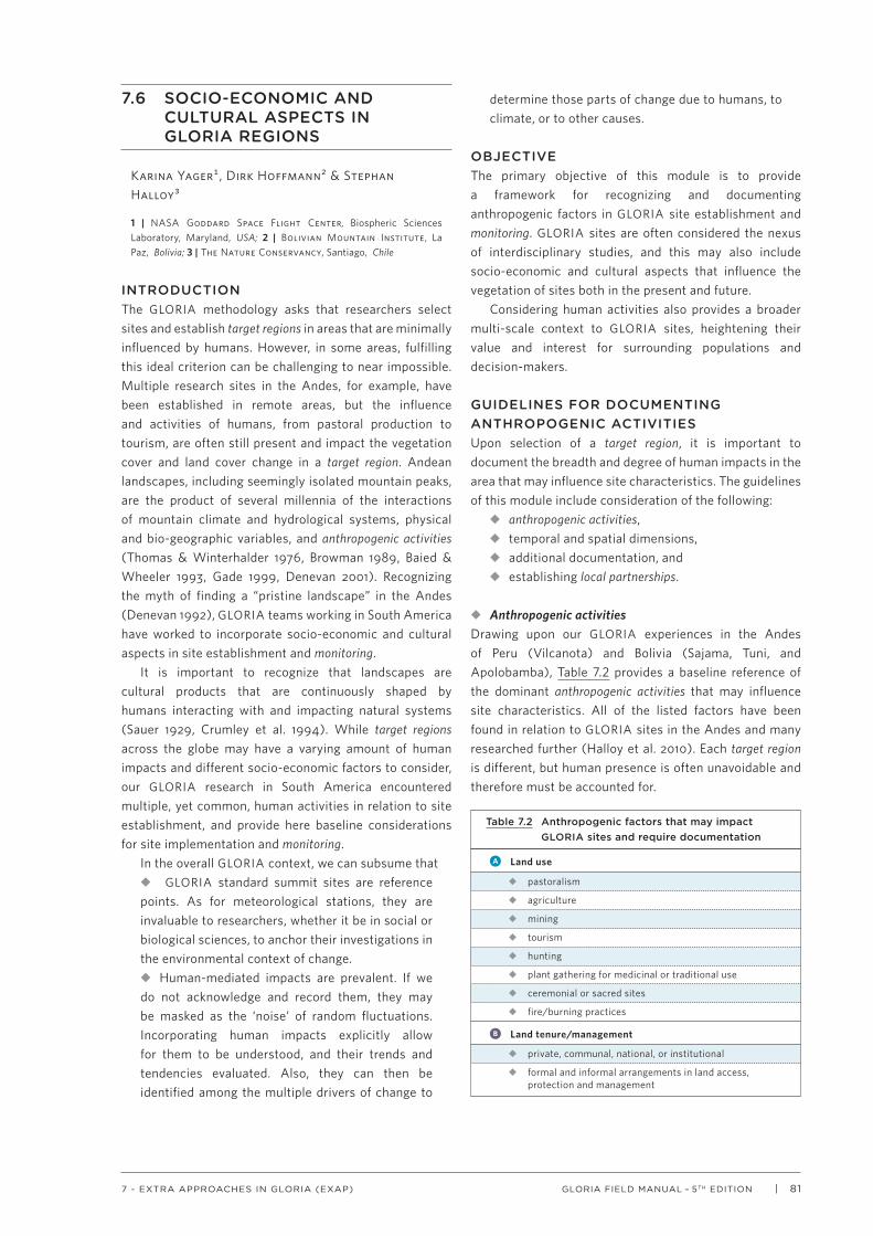
| 81GLORIA FIELD MANUAL – 5TH  EDITION7 - EXTRA APPROACHES IN GLORIA (EXAP)

7.6 SOCIO-ECONOMIC AND CULTURAL ASPECTS IN GLORIA REGIONS

Karina Yager¹, Dirk Hoffmann² & Stephan Halloy³

1 | NASA Goddard Space Flight Center, Biospheric Sciences Laboratory, Maryland, USA; 2 | Bolivian Mountain Institute, La Paz, Bolivia; 3 | The Nature Conservancy, Santiago, Chile

INTRODUCTIONThe GLORIA methodology asks that researchers select sites and establish target regions in areas that are minimally influenced by humans. However, in some areas, fulfilling this ideal criterion can be challenging to near impossible. Multiple research sites in the Andes, for example, have been established in remote areas, but the influence and activities of humans, from pastoral production to tourism, are often still present and impact the vegetation cover and land cover change in a target region. Andean landscapes, including seemingly isolated mountain peaks, are the product of several millennia of the interactions of mountain climate and hydrological systems, physical and bio-geographic variables, and anthropogenic activities (Thomas & Winterhalder 1976, Browman 1989, Baied & Wheeler 1993, Gade 1999, Denevan 2001). Recognizing the myth of finding a “pristine landscape” in the Andes (Denevan 1992), GLORIA teams working in South America have worked to incorporate socio-economic and cultural aspects in site establishment and monitoring.

It is important to recognize that landscapes are cultural products that are continuously shaped by humans interacting with and impacting natural systems (Sauer 1929, Crumley et al. 1994). While target regions across the globe may have a varying amount of human impacts and different socio-economic factors to consider, our GLORIA research in South America encountered multiple, yet common, human activities in relation to site establishment, and provide here baseline considerations for site implementation and monitoring.

In the overall GLORIA context, we can subsume thatu GLORIA standard summit sites are reference points. As for meteorological stations, they are invaluable to researchers, whether it be in social or biological sciences, to anchor their investigations in the environmental context of change. u Human-mediated impacts are prevalent. If we do not acknowledge and record them, they may be masked as the ‘noise’ of random fluctuations. Incorporating human impacts explicitly allow for them to be understood, and their trends and tendencies evaluated. Also, they can then be identified among the multiple drivers of change to

determine those parts of change due to humans, to climate, or to other causes.

OBJECTIVEThe primary objective of this module is to provide a framework for recognizing and documenting anthropogenic factors in GLORIA site establishment and monitoring. GLORIA sites are often considered the nexus of interdisciplinary studies, and this may also include socio-economic and cultural aspects that influence the vegetation of sites both in the present and future.

Considering human activities also provides a broader multi-scale context to GLORIA sites, heightening their value and interest for surrounding populations and decision-makers.

GUIDELINES FOR DOCUMENTING ANTHROPOGENIC ACTIVITIESUpon selection of a target region, it is important to document the breadth and degree of human impacts in the area that may influence site characteristics. The guidelines of this module include consideration of the following:

u anthropogenic activities, u temporal and spatial dimensions, u additional documentation, and u establishing local partnerships.

u Anthropogenic activitiesDrawing upon our GLORIA experiences in the Andes of Peru (Vilcanota) and Bolivia (Sajama, Tuni, and Apolobamba), Table 7.2 provides a baseline reference of the dominant anthropogenic activities that may influence site characteristics. All of the listed factors have been found in relation to GLORIA sites in the Andes and many researched further (Halloy et al. 2010). Each target region is different, but human presence is often unavoidable and therefore must be accounted for.

Table 7.2 Anthropogenic factors that may impact GLORIA sites and require documentation

A Land use

u pastoralism

u agriculture

u mining

u tourism

u hunting

u plant gathering for medicinal or traditional use

u ceremonial or sacred sites

u fire/burning practices

B Land tenure/management

u private, communal, national, or institutional

u formal and informal arrangements in land access, protection and management

82 | GLORIA FIELD MANUAL – 5TH  EDITION7 - EXTRA APPROACHES IN GLORIA (EXAP)

Some anthropogenic factors may require further investigation in order to properly assess the amount of impact they may have in a target region or on site characteristics. For example, pastoralism is particularly common in the Andes, and both domesticated and wild grazing animals can influence species richness and cover in a target region (Yager et al. 2008a, Patty et al. 2010). Often evidence of animal grazers is documented at GLORIA sites during site establishment and survey, including presence of animal dung/droppings or clipping (i.e. grazing) of vegetation. If there is abundant evidence of animals disturbing the site, it may be of interest to conduct a more thorough study of the number of animals accessing the site, and to further investigate local pasture management or rotation practices. Pasture management may often include intentional or non-intentional burning or fire practices that will certainly influence vegetation succession. These activities may require interviews with locals and field monitoring (including camera installation or on-going surveys).

Also prevalent in the Andes is the use of a target region by locals and visitors for tourism, plant gathering, and ceremonial practices. Therefore, the amount of foot traffic in a region may vary throughout the year and over time. Some may come infrequently or seasonally, accessing the area as a corridor for photography, trekking, or exploration, while others may come regularly to gather rare plants for medicinal purposes, or to visit high mountain areas for ceremonial purposes. Below are photographs that show some of the common human activities (Fig.  7.12) as occurring in the GLORIA target region of Sajama National Park, Bolivia.

u Temporal and spatial dimensionsIt is important to also recognize the temporal and spatial dimensions of human impacts. In particular, one must consider the past, present, and potential impacts of humans while documenting and monitoring sites. Even if human presence is not highly visible or noted during site establishment, it does not guarantee that sites may not be subject to the impacts of social changes in the future. Sites

might have been impacted in the past in ways which are not necessarily obvious to the uninformed researcher. For example, past large-scale extraction of yareta (Azorella compacta) cushions and queñua (Polylepis tarapacana) trees for fuel used in mines and railroads has left whole landscapes devoid of these plants, which were originally part of the local alpine vegetation.

While mountain and alpine areas, from the Alps to the Andes, are recognized and even valued for their isolation, thus making them ideal “natural laboratories” for the study of natural systems and minimally influenced vegetation (Barry 1994, Grabherr et al. 2000, Körner 2003); it is also recognized that humans have inhabited and influenced alpine ecological systems for generations (Ellenberg 1979, Netting 1981, 1990, Gade 1999), alongside climate change in recent years (Grabherr et al. 1994, Erschbamer et al. 2006, Gottfried et al. 2012, Pauli et al. 2012), and that both climate change and humans are expected to have an even greater impact on alpine regions in the future (Beniston 1994, Vuille et al. 2008, Seimon et al. 2009). In the Andes, even the “protected areas” have many indigenous communities that continue to live in the park and utilize the resources, including alpine vegetation. Thus, the human factor must be considered along with the climate change factor over space and time.

Climate change and ongoing social changes (from population growth to competition over land or resources) may further influence future access and the movement of people and animals into a region. Production zones of a particular ecological tier may become overcrowded or unproductive due to climate or social change, and cause the displacement or upward movement of peoples and animals to access, occupy, and utilize the resources at higher elevations in mountain regions. Thus, it is important to consider and document the varying levels of production and people in a particular target region. Drawing again on the example of GLORIA in Sajama, the primary production zones in a target region were documented, including the elevational tiers of production and dominant species (Yager 2009, Beck et al. 2010a). Interdisciplinary studies

Fig. 7.12 Photographs of anthropogenic activities in a GLORIA target region, Sajama, Bolivia. (Left: Burning, Center: Pathways, Right: Cultural Site)

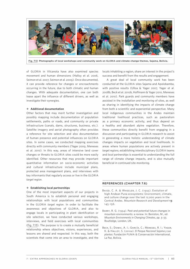
| 83GLORIA FIELD MANUAL – 5TH  EDITION7 - EXTRA APPROACHES IN GLORIA (EXAP)

of GLORIA in Vilcanota have also examined species movement and human dimensions (Halloy et al. 2006, Seimon et al. 2007, Seimon et al. 2009). Once documented, it can provide reference for changes or encroachments occurring in the future, due to both climatic and human changes. With adequate documentation, one can both tease apart the influence of different drivers, as well as investigate their synergies.

u Additional documentationOther factors that may merit further investigation and possibly mapping include documentation of population settlements, paths or roads, and community or private infrastructure (canals, dams, structures, business, etc.). Satellite imagery and aerial photography often provides a reference for site selection and also documentation of human presence and potential influences on GLORIA sites. In some cases, we conducted mapping exercises directly with community members (Yager 2009, Meneses et al. 2010). In this way, areas of intensive land cover changes or threats to GLORIA sites could be more easily identified. Other resources that may provide important quantitative information on socio-economic activities and cultural infrastructure include municipal plans, protected area management plans, and interviews with key informants that regularly access or live in the GLORIA target region.

u Establishing local partnershipsOne of the most important aspects of our projects in South America is to establish personal and engaging relationships with local populations and communities in the GLORIA target region. In order to facilitate the awareness and objectives of GLORIA, and also to engage locals in participating in plant identification or site selection, we have conducted various workshops, interviews, and field exercises with local communities (Fig. 7.13). The purpose is to create a mutually beneficial relationship where objectives, visions, experiences, and lessons are shared and respected. In this way, both the scientists that come into an area to investigate, and the

locals inhabiting a region, share an interest in the project’s success and benefit from the results and engagement.

A great deal of local community work has been conducted at the GLORIA sites Sajama and Apolobamba, with positive results (Ulloa & Yager 2007, Yager et al. 2008b, Beck et al. 2010b, Hoffmann & Yager 2010, Meneses et al. 2010). Park guards and community members have assisted in the installation and monitoring of sites, as well as sharing in identifying the impacts of climate change from both a scientific and experiential perspective. Many local indigenous communities in the Andes maintain traditional livelihood practices, such as pastoralism as a primary economic activity, and thus depend on a healthy and abundant alpine vegetation. Therefore, these communities directly benefit from engaging in a discussion and participating in GLORIA research to assist in generating a more holistic understanding of climate changes impacts on vegetation and local livelihoods. In areas where human populations are actively present in target regions, establishing interdisciplinary GLORIA teams and local partnerships is essential to understanding the full range of climate change impacts, and is also mutually beneficial in continued site monitoring.

Fig. 7.13 Photographs of local workshops and community work on GLORIA and climate change themes, Sajama, Bolivia.

REFERENCES (CHAPTER 7.6)

Baied, C. A. & Wheeler, J . C. ( 1 9 9 3 ) . Evolution of high Andean Puna ecosystems: Environment, climate, and culture change over the last 12,000 years in the Central Andes. Mountain Research and Development 13 : 145-156.

Barry, R. G. (1994). Past and potential future changes in mountain environments: a review. In: Beniston, M., ed. Mountain Environments in Changing Climates, pp. 3-33. Routledge, London, UK.

Beck, S.; Domic, A. I.; García, C.; Meneses, R. I.; Yager, K. & Halloy, S. (2010a). El Parque Nacional Sajama y sus plantas. Fundación PUMA & Conservación International, La Paz, Bolivia.

84 | GLORIA FIELD MANUAL – 5TH  EDITION7 - EXTRA APPROACHES IN GLORIA (EXAP)

Beck, S.; Yager, K.; Meneses, R. I.; Halloy, S.; Domic, A. I. & Garcia, C. (2010b). GLORIA sites in the high Andes of Bolivia: A multi-disciplinary assessment. 6th International GLORIA (Global Observation Research Initiative in Alpine Environments) Meeting, Perth, Scotland, UK.

Beniston, M. (1994). Mountain environments in changing climates. Routledge, London, UK.

Browman, D. L. (1989). Origins and development of Andean pastoralism: an overview of the the past 6000 years. In: Clutton-Brock, J., ed. The Walking Larder: Patterns of domestication, pastoralism, and predation, pp. 257-268. Unwin Hyman, London, UK.

Crumley, C. L.; Gunn, J. D.; Hassan, F. A.; Ingerson, A. E.; Marquardt, W. H.; McGovern, T. H.; Patterson, T. C.; Schmidt, P. R. & Winterhalder, B. P. (1994). Historical ecology: Cultural knowledge and changing landscapes. School of American Research Press, Santa Fe, USA.

Denevan, W. M. (1992). The pristine myth - the landscape of the America in 1492. Annals of the Association of American Geographers 82: 369-385.

Denevan, W. M. (2001). Cultivated landscapes of native Amazonia and the Andes. Oxford University Press, Oxford, UK.

Ellenberg, H. (1979). Man’s influence on tropical mountain ecosystems in South America. Journal of Ecology 67: 401-416.

Erschbamer, B.; Mallaun, M. & Unterluggauer, P. (2006). Plant diversity along altitudinal gradients in the Southern and Central Alps of South Tyrol and Trentino (Italy). Gredleriana 6: 47-68.

Gade, D. W. (1999). Nature and culture in the Andes. University of Wisconsin Press, Madison, Wisconsin, USA.

Gottfried, M.; Pauli, H.; Futschik, A.; Akhalkatsi, M.; Barancok, P.; Benito Alonso, J. L.; Coldea, G.; Dick, J.; Erschbamer, B.; Fernández Calzado, M. R.; Kazakis, G.; Krajci, J.; Larsson, P.; Mallaun, M.; Michelsen, O.; Moiseev, D.; Moiseev, P.; Molau, U.; Merzouki, A.; Nagy, L.; Nakhutsrishvili, G.; Pedersen, B.; Pelino, G.; Puscas, M.; Rossi, G.; Stanisci, A.; Theurillat, J.-P.; Tomaselli, M.; Villar, L.; Vittoz, P.; Vogiatzakis, I. & Grabherr, G. (2012). Continent-wide response of mountain vegetation to climate change. Nature Climate Change 2: 111-115.

Grabherr, G.; Gottfried, M. & Pauli, H. (1994). Climate effects on mountain plants. Nature 369: 448-448.

Grabherr, G.; Gottfried, M. & Pauli, H. (2000). GLORIA: A Global Observation Research Initiative in Alpine Environments. Mountain Research and Development 20: 190-191.

Halloy, S.; Seimon, A. & Yager, K. (2006). Multidimensional (climate, biodiversity, socioeconomics, agriculture) context of changes in land use in the Vilcanota

watershed, Peru. In: Spehn, E. M.; Liberman, M. & Körner, C., eds. Land Use Change and Mountain Biodiversity, pp. 323-337. CRC Press, Fort Lauderdale, USA.

Halloy, S.; Yager, K.; García, C.; Beck, S.; Carilla, J.; Tupayachi, A.; Jácome, J.; Meneses, R. I.; Farfán, J.; Seimon, A.; Seimon, T.; Rodriguez, P.; Cuello, S. & Grau, A. (2010). South America: Climate monitoring and adaptation integrated across regions and disciplines. In: Settele, J.; Penev, L. D.; Georgiev, T. A.; Grabaum, R.; Grobelnik, V.; Hammen, V.; Klotz, S.; Kotarac, M. & Kuehn, I., eds. Atlas of biodiversity risk, pp. 90-95. Pensoft Publishers, Sofia, Bulgaria.

Hoffmann, D. & Yager, K. (2010). Identification and incorporation of socio-economic and cultural aspects of site implementation and monitoring. 6th International GLORIA (Global Observation Research Initiative in Alpine Environments) Meeting, Perth, Scotland, UK.

Körner, C. (2003). Alpine plant life: functional plant ecology of high mountain ecosystems. Springer, Berlin, Germany.

Meneses, R. I.; Yager, K.; Canqui, F. & Beck, S. (2010). Pastoralism of the high puna of Bolivia: local perceptions of climate change and the challenged of maintain tradition. Global Change and the World’s Mountains Conference, Perth, Scotland, UK.

Netting, R. M. (1981). Balancing on an Alp: Ecological change & continuity in a Swiss mountain community. Press Syndicate of the University of Cambridge, Cambridge, New York (USA) and Melbourne (Australia).

Netting, R. M. (1990). Links and boundaries: Reconsidering the alpine village as ecosystem. In: Moran, E. F., ed. The ecosystem approach, pp. 229-245. University of Michigan Press, Ann Arbor, USA.

Patty, L.; Halloy, S. R. P.; Hiltbrunner, E. & Körner, C. (2010). Biomass allocation in herbaceous plants under grazing impact in the high semi-arid Andes. Flora (Jena) 205: 695-703.

Pauli, H.; Gottfried, M.; Dullinger, S. ; Abdaladze, O.; Akhalkatsi, M.; Benito Alonso, J. L. ; Coldea, G.; Dick, J. ; Erschbamer, B. ; Fernández Calzado, R.; Ghosn, D.; Holten, J. I . ; Kanka, R. ; Kazakis, G.; Kollár, J. ; Larsson, P. ; Moiseev, P. ; Moiseev, D.; Molau, U.; Molero Mesa, J. ; Nagy, L. ; Pelino, G.; Puşcaş, M.; Rossi, G.; Stanisci, A.; Syverhuset, A. O.; Theurillat, J.-P. ; Tomaselli , M.; Unterluggauer, P. ; Villar, L. ; Vittoz, P. & Grabherr, G. (2012) . Recent plant diversity changes on Europe’s mountain summits. Science 336 : 353-355.

Sauer, C. (1929). The morphology of landscape. University of California Publications in Geography II (1919-1929) 2: 19-53.

Seimon, A.; Yager, K.; Seimon, T.; Schmidt, S.; Grau, A.; Beck, S.; García, C.; Tupayachi, A.; Sowell, P.; Touval, J. & Halloy, S. (2009). Changes in biodiversity patterns in the high Andes – understanding the consequences and seeking adaption to global change. Mountain Forum Bulletin 4: 25-27.

| 85GLORIA FIELD MANUAL – 5TH  EDITION7 - EXTRA APPROACHES IN GLORIA (EXAP)

Seimon, T. A.; Seimon, A.; Daszak, P.; Halloy, S. R. P.; Schloegel, L. M.; Aguilar, C. A.; Sowell, P.; Hyatt, A. D.; Konecky, B. & Simmons, J. E. (2007). Upward range extension of Andean anurans and chytridiomycosis to extreme elevations in response to tropical deglaciation. Global Change Biology 13: 288-299.

Thomas, R. B. & Winterhalder, B. P. (1976). Physical and biotic environment of southern highland Peru. In: Baker, P. T. & Little, M. A., eds. Man in the Andes: A multidisciplinary study of high-altitude Quechua, pp. 21-59. Dowden, Hutchison & Ross, Inc., Stroudsburg, USA.

Ulloa, D. & Yager, K. (2007). Memorias del taller: “Cambio climático: percepción local y adaptaciones en el Parque Nacional Sajama”. p. 42. Comunidad de Sajama, Lagunas, Caripe, Manasaya y Papelpampa, Sajama, Bolivia.

Vuille, M.; Francou, B.; Wagnon, P.; Juen, I.; Kaser, G.; Mark, B. G. & Bradley, R. S. (2008). Climate change and tropical Andean glaciers: Past, present and future. Earth-Science Reviews 89: 79-96.

Yager, K.; Resnikowski, H. & Halloy, S. (2008a). Grazing and climatic variability in Sajama National Park, Bolivia. Pirineos 163: 97-109.

Yager, K.; Ulloa, D. & Halloy, S. (2008b). Conducting an interdisciplinary workshop on climate change: facilitating awareness and adaptation in Sajama National Park, Bolivia. In: Mannke, F. & Filho, W. L., eds. Interdisciplinary aspects of climate change, pp. 327-342. University of Applied Sciences, Hamburg, Germany.

Yager, K. A. (2009). A herder’s landscape: Deglaciation, desiccation and managing green pastures in the Andean puna. Yale University, New Haven, USA.

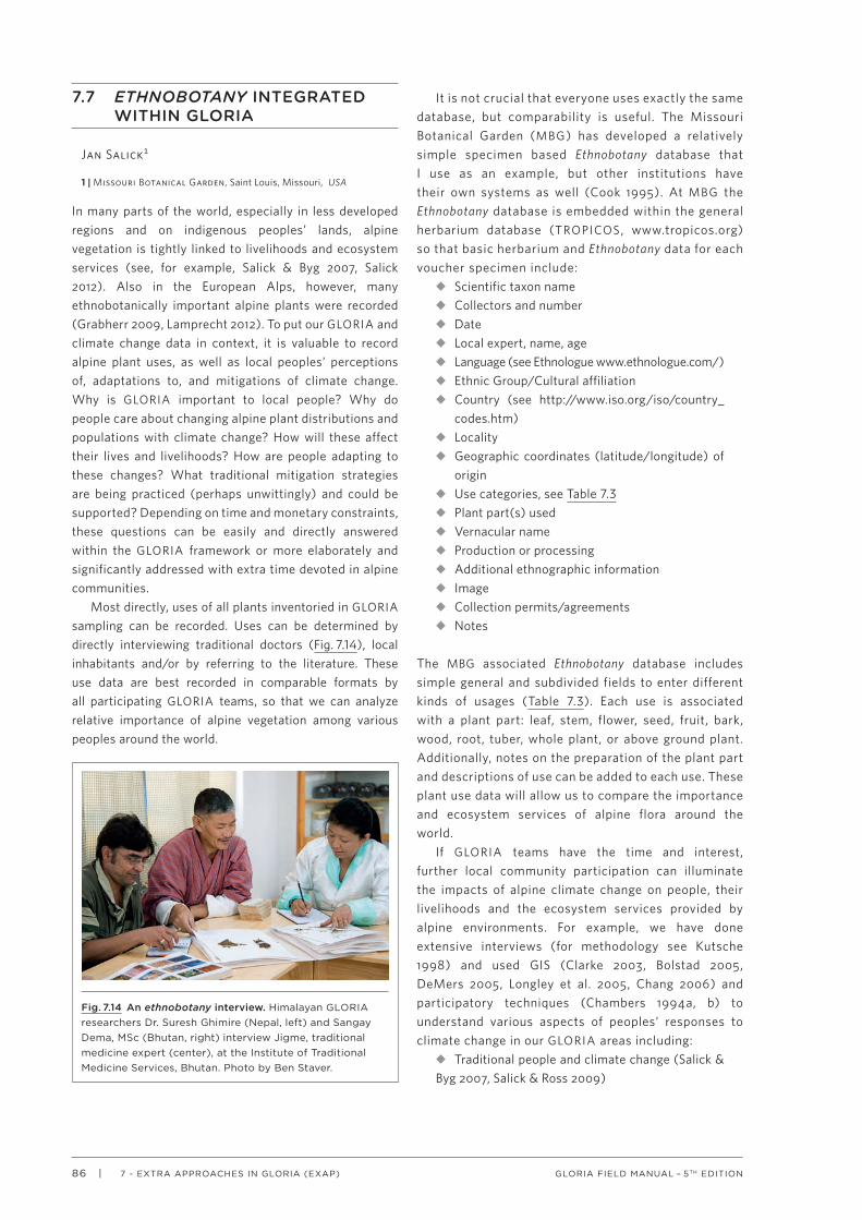
86 | GLORIA FIELD MANUAL – 5TH  EDITION7 - EXTRA APPROACHES IN GLORIA (EXAP)

7.7 ETHNOBOTANY INTEGRATED WITHIN GLORIA

Jan Salick¹

1 | Missouri Botanical Garden, Saint Louis, Missouri, USA

In many parts of the world, especially in less developed regions and on indigenous peoples’ lands, alpine vegetation is tightly linked to livelihoods and ecosystem services (see, for example, Salick & Byg 2007, Salick 2012). Also in the European Alps, however, many ethnobotanically important alpine plants were recorded (Grabherr 2009, Lamprecht 2012). To put our GLORIA and climate change data in context, it is valuable to record alpine plant uses, as well as local peoples’ perceptions of, adaptations to, and mitigations of climate change. Why is GLORIA important to local people? Why do people care about changing alpine plant distributions and populations with climate change? How will these affect their lives and livelihoods? How are people adapting to these changes? What traditional mitigation strategies are being practiced (perhaps unwittingly) and could be supported? Depending on time and monetary constraints, these questions can be easily and directly answered within the GLORIA framework or more elaborately and significantly addressed with extra time devoted in alpine communities.

Most directly, uses of all plants inventoried in GLORIA sampling can be recorded. Uses can be determined by directly interviewing traditional doctors (Fig. 7.14), local inhabitants and/or by referring to the literature. These use data are best recorded in comparable formats by all participating GLORIA teams, so that we can analyze relative importance of alpine vegetation among various peoples around the world.

It is not crucial that everyone uses exactly the same database, but comparability is useful. The Missouri Botanical Garden (MBG) has developed a relatively simple specimen based Ethnobotany database that I use as an example, but other institutions have their own systems as well (Cook 1995). At MBG the Ethnobotany database is embedded within the general herbarium database (TROPICOS, www.tropicos.org) so that basic herbarium and Ethnobotany data for each voucher specimen include:

u Scientific taxon nameu Collectors and numberu Dateu Local expert, name, ageu Language (see Ethnologue www.ethnologue.com/)u Ethnic Group/Cultural affiliationu Country (see http://www.iso.org/iso/country_ codes.htm)u Localityu Geographic coordinates (latitude/longitude) of originu Use categories, see Table 7.3u Plant part(s) usedu Vernacular nameu Production or processingu Additional ethnographic informationu Imageu Collection permits/agreementsu Notes

The MBG associated Ethnobotany database includes simple general and subdivided fields to enter different kinds of usages (Table 7.3). Each use is associated with a plant part: leaf, stem, flower, seed, fruit, bark, wood, root, tuber, whole plant, or above ground plant. Additionally, notes on the preparation of the plant part and descriptions of use can be added to each use. These plant use data will allow us to compare the importance and ecosystem services of alpine flora around the world.

If GLORIA teams have the time and interest, further local community participation can illuminate the impacts of alpine climate change on people, their livelihoods and the ecosystem services provided by alpine environments. For example, we have done extensive interviews (for methodology see Kutsche 1998) and used GIS (Clarke 2003, Bolstad 2005, DeMers 2005, Longley et al. 2005, Chang 2006) and participatory techniques (Chambers 1994a, b) to understand various aspects of peoples’ responses to climate change in our GLORIA areas including:

u Traditional people and climate change (Salick & Byg 2007, Salick & Ross 2009)

Fig. 7.14 An ethnobotany interview. Himalayan GLORIA researchers Dr. Suresh Ghimire (Nepal, left) and Sangay Dema, MSc (Bhutan, right) interview Jigme, traditional medicine expert (center), at the Institute of Traditional Medicine Services, Bhutan. Photo by Ben Staver.

| 87GLORIA FIELD MANUAL – 5TH  EDITION7 - EXTRA APPROACHES IN GLORIA (EXAP)

u Tibetans’ perceptions of climate change (Byg & Salick 2009, Salick et al. 2012)u Traditional agro-pastoral land use and change (Salick et al. 2005, Salick & Moseley 2012)u Tibetan sacred sites conserve alpine biodiversity (Anderson et al. 2005, Salick et al. 2007)u Tibetan doctors and villagers collect medicinal plants in high alpine meadows (Salick et al. 2004, Law & Salick 2005, Salick et al. 2006, Law & Salick 2007, Salick et al. 2009, Byg et al. 2010, Salick et al. 2012)u Tibetan cosmology of climate change (Salick & Moseley 2012)u Climate change affects Tibetan culture, land use, health, medicine, agriculture, and forestry (Salick 2012, Salick et al. 2012)u Using traditional knowledge, Tibetans creatively adapt to climate change (Salick et al. 2012)

Added to GLORIA’s intensive ecological monitoring, these cultural data provide a powerful platform from which to analyze the dynamics of coupled natural and human systems in response to global climate change. Additionally, GLORIA data are given meaning and relevance to local people with whom many of us work.

Table 7.3 Use categories of Missouri Botanical Garden Ethnobotany database (under TROPICOS, www.tropicos.org)

A Food – human u Infections, parasites, fungi G Cultural Uses

u Beverages u Inflammation and pain u Handicrafts (non-fiber)

u Condiments, herbs, spices u Poisons and antidotes u Recreation, games, sports, toys

u Fruits and vegetables u Zoopharmacognosy u Religion

u Legumes and pulses u "Humors" u Accessories, cosmetics, jewelry

u Grains and rice u Belief systems u Musical instruments, art

u Root and tuber carbohydrates u General, non-specific symptoms u Psychoactive drugs

u Nuts u Other/NA u Other/NA

u Additives

u Other/NA D Chemicals H Constructions/Structural materials

u Latex, rubber u Timber

B Food – animal u Resins, non-edible gums u Furniture

u Fodder, forage, graze, silage u Oils (non-edible), waxes, soaps u Building materials

u Browse u Dyes, paints, colors u Tools, utensils

u Invertebrate food u Tannins, flavonoids u Transportation

u Fruits u Aromatics u Other/NA

u Other/NA u Solvents

u Adhesives I Environmental

C Medicines – human & veterinary u Other/NA u Barriers, boundaries

u Blood and circulatory system u Erosion control

u Dental E Fuels u Fertilizers, soil improvement

u Digestive system u Firewood, charcoal u Ornamentals

u Endocrine system (hormones) u Oils, alcohols, resins, waxes u Pollution control

u Female and male reproductive systems u Other/NA u Pest control

u Urinary system u Other/NA

u Immune system F Fibers

u Metabolic system, fevers, nutrition u Cloth, clothing, apparel, thread J Other

u Muscular-skeletal systems u Paper u Research

u Nervous system and mental health u Baskets, fiber, containers, fiber u Genetic resources

u Respiratory system household goods, fiber handicrafts

u Sensory systems u Rope, string, netting K Notes: detail on use(s)

u Skin and related tissue u Other/NA

88 | GLORIA FIELD MANUAL – 5TH  EDITION7 - EXTRA APPROACHES IN GLORIA (EXAP)

REFERENCES (CHAPTER 7.7)

Anderson, D. M.; Salick, J.; Moseley, R. K. & Ou, X. K. (2005). Conserving the sacred medicine mountains: A vegetation analysis of Tibetan sacred sites in Northwest Yunnan. Biodiversity and Conservation 14: 3065-3091.

Bolstad, P. (2005). GIS Fundamentals: A First Text on Geographic Information Systems. Eider Press, White Bear Lake, Montana, USA.

Byg, A. & Salick, J. (2009). Local perspectives on a global phenomenon – Climate change in eastern Tibetan villages. Global Environmental Change-Human and Policy Dimensions 19: 156-166.

Byg, A.; Salick, J. & Law, W. (2010). Medicinal plant knowledge among lay people in five eastern Tibet villages. Human Ecology 38: 177-191.

Chambers, R. (1994a). The origins and practice of participatory rural appraisal. World Development 22: 953-969.

Chambers, R. (1994b). Participatory rural appraisal (PRA) - Analysis of experience. World Development 22: 1253-1268.

Chang, K.-T. (2006). Introduction to Geographic Information Systems. McGraw-Hill Higher Education, Boston.

Clarke, K. C. (2003). Getting started with geographic information systems. Prentice Hall, Upper Saddle River, NJ.

Cook, F. E. M. (1995). Economic botany data collection standard. Prepared for the International working group on taxonomic databases for plant sciences (TDWG). Royal Botanical Gardens, Kew.

DeMers, M. N. (2005). Fundamentals of geographic information systems. John Wiley & Sons, New York.

Grabherr, G. (2009). Biodiversity in the high ranges of the Alps: Ethnobotanical and climate change perspectives. Global Environmental Change—Human and Policy Dimensions 19: 167-172.

Kutsche, P. (1998). Field ethnography: A manual for doing cultural anthropology. Prentice Hall, Upper Saddle River, NJ.

Lamprecht, A. (2012) . Ethnobotanische Aspekte der Hochgebirgsflora der Ostalpen: Dokumentation der für Menschen nutzbaren Gefäßpflanzen in den GLORIA-Untersuchungsgebieten Hochschwab, Schrankogel und Latemar. Diploma thesis, University of Vienna, Austria.

Law, W. & Salick, J. (2005). Human-induced dwarfing of Himalayan snow lotus, Saussurea laniceps (Asteraceae). Proceedings of the National Academy of Sciences of the United States of America 102: 10218-10220.

Law, W. & Salick, J. (2007). Comparing conservation priorities for useful plants among botanists and tibetan doctors. Biodiversity and Conservation 16: 1747-1759.

Longley, P. A.; Goodchild, M. F.; Maguire, D. J. & Rhind, D. W. (2005). Geographic information systems and science. John Wiley & Sons Ltd, Chichester, West Sussex, UK.

Salick, J. (2012). Indigenous peoples conserving, managing, and creating biodiversity. In: Gepts, P.; Famula, T. R.; Bettinger, R. L.; Brush, S. B.; Damania, A. B.; McGuire, P. E. & Qualset, C. O., eds. Biodiversity in agriculture: Domestication, evolution, and sustainability, pp. 426-444. Cambridge University Press, New York.

Salick, J.; Amend, A.; Anderson, D.; Hoffmeister, K.; Gunn, B. & Fang, Z. (2007). Tibetan sacred sites conserve old growth trees and cover in the eastern Himalayas. Biodiversity and Conservation 16: 693-706.

Salick, J.; Anderson, D.; Woo, J.; Sherman, R.; Cili, N.; Ana & Dorje, S. (2004). Tibetan ethnobotany and gradient analyses: Menri (Medicine Mountains), eastern Himalayas. Millenium ecosystem assessment. Alexandria, Egypt.

Salick, J. & Byg, A. (2007). Indigenous peoples and climate change. Environmental Change Institute, University of Oxford, Symposium report, 12-13 April 2007. Tyndall Centre for Climate Change Research, Oxford, UK.

Salick, J.; Byg, A.; Amend, A.; Gunn, B.; Law, W. & Schmidt, H. (2006). Tibetan medicine plurality. Economic Botany 60: 227-253.

Salick, J.; Byg, A. & Bauer, K. (2012). Contemporary Tibetan cosmology of climate change. Journal for the Study of Religion, Nature and Culture 6: 447-476.

Salick, J.; Fang, Z. & Byg, A. (2009). Eastern Himalayan alpine plant ecology, Tibetan ethnobotany, and climate change. Global Environmental Change—Human and Policy Dimensions 19: 147-155.

Salick, J. & Moseley, R. K. (2012). Khawa Karpo: Tibetan traditional knowledge and biodiversity conservation. Missouri Botanical Garden Press, St. Louis.

Salick, J. & Ross, N. (2009). Traditional peoples and climate change: Introduction. Special Issue: Global Environmental Change—Human and Policy Dimensions 19: 137-139.

Salick, J.; Yang, Y. P. & Amend, A. (2005). Tibetan land use and change near Khawa Karpo, eastern Himalayas. Economic Botany 59: 312-325.

| 89GLORIA FIELD MANUAL – 5TH  EDITIONGLOSSARY OF TERMS USED IN THE MANUAL

››  All terms listed in this glossary are written in italics throughout this manual.

1-m² quadrat: Permanent 1 m × 1 m quadrats for detailed vegetation recording positioned at the four corner positions within the 3 m × 3 m quadrat clusters.

3 m × 3 m quadrat cluster: A 3 m × 3 m square positioned in each of the four main geographic directions referring to the highest summit point (HSP) with its lower side at the 5-m level below the HSP.

3 m × 3 m grid: Grids constructed of flexible measuring tapes with 3 × 3 subdivisions (i.e. nine 1-m² quadrats); see Fig. AI.1 in Annex I.

5-m level: The elevation level at the 5-m contour line below the highest summit point (HSP).

5-m summit area: The upper summit area, divided into four summit area sections for recording. This area reaches the 5-m level at the two lower corner points (p5m-...) of each 3 m × 3 m quadrat cluster. Between the quadrat clusters, this area usually lies above the 5-m level because the corner points are connected by the shortest straight lines possible. The 5-m summit area also includes the quadrats of the 3 m × 3 m quadrat clusters.

10-m level: The elevation level at the 10-m contour line below the highest summit point (HSP).

10-m summit area: The lower summit area, divided into four summit area sections for sampling. The lower boundary of this area is delimited by four corner points (p10m-.) at the 10-m level in each of the four cardinal directions, which are connected by the shortest straight lines possible. The 10-m summit area lies between this line and the lower limit of the 5-m summit area.

10 m × 10 m squares: A supplementary design and recording procedure within the summit area. 10 m × 10 m squares are established in each cardinal direction with their mid-, upper and lower points on the intersection line of the respective cardinal direction, where the

mid-point is one of the lower corners of the 3 m × 3 m quadrat cluster. In each square a total of 400 points are sampled by applying the line-pointing method along 20 parallel strings. Finally, the remaining rarer species not recorded during line-pointing are inventoried.

16-quadrat area: The sum of all 1-m² quadrats of a summit; these are 16 in number (four per quadrat cluster in four clusters, one in each cardinal direction).

Abundance categories: Abundance classes along an ordinal scale used for the estimation of species abundance in SASs. Five abundance categories are distinguished: r! (very rare), r (rare), s (scattered), c (common), d (dominant). See chapter 4.2 for definitions.

Alpine life zone: The mountain terrain starting at the low-temperature determined treeline ecotone and extending upwards. It comprises the area where any low-stature vegetation or scattered plant individuals between the climatic treeline ecotone and the highest mountain tops occur. The term is also applied to the entirety of high mountain biomes world-wide (compare Körner 2003).

Alpine-nival ecotone (or subnival zone): The transition between the alpine zone and the nival zone; it may coincide with the lower permafrost limit.

Alpine zone: The zone between the treeline and the upper limit of closed vegetation. Here, the vegetation is a significant part of the landscape and its physiognomy and plant cover is usually >20–40%. In some mountain regions it is subdivided into a lower alpine zone dominated by dwarf-shrub communities, and an upper alpine zone dominated by grassland communities (Nagy & Grabherr 2009).

Altitudinal index: Indicates the average vertical distribution of a plant species across a set of four summit areas of a GLORIA target region in a specific year of observation. It is computed by first defining the relative altitude of each summit in metres above the altitude of the lowest summit and second, by weighting these relative altitudes by the species’ frequencies on the respective summits (i.e. the presence/

absence of the species in the eight summit area sections per summit). Finally the altitudinal index of a species is calculated as the weighted average altitude of the species’ distribution across the four summit sites (Pauli et al. 2012).

Altitudinal species profile: Describes the vertical distribution of a plant species across vegetation belts by its lower (AL) and upper (AU) distribution margin, as well as its distribution centre (AC) (Gottfried et al. 2012). An AL-AC-AU profile is expressed as vegetation belts: montane (mo), treeline ecotone (tl), alpine (al), nival (ni), indifferent (id). E.g. mo-tl-al stands for a species which is centred at the treeline ecotone but extends into both the montane and the alpine belt, tl-id-al would mean the species is equally distributed from the treeline ecotone to the alpine belt. Extreme outposts at lower elevations should not be considered.

Altitudinal species rank: The vertical distribution of plant species defined by Gottfried et al. (2012) as six rank classes. Each rank class comprises a set of similar altitudinal species profiles, following the classical central European concept of vegetation belts. The ranks are defined as: (1) species with a nival distribution centre, (2) alpine to nival species that do not descend to the treeline, (3) alpine centred species which do not descend to the montane belt, (4) alpine centred species that descend to the montane belt and species indifferently distributed from the treeline to the alpine belt, (5) species centred in the treeline ecotone or indifferently distributed from the montane to the alpine belt, (6) species with a montane-centred distribution or indifferent from the montane belt to the treeline.

Anthropogenic activities: Impacts of human activities such as land use through, e.g., pastoralism, agriculture, mining, tourism, burning practices, or through land tenure may alter alpine vegetation and biodiversity patterns. Therefore, type, spatial dimension as well as temporal dimensions (impacts may change over time due to socio-economic constraints) are documented as an extra approach in some GLORIA target regions (chapter 7.6).

GLOSSARY OF TERMS USED IN THE MANUAL

90 | GLORIA FIELD MANUAL – 5TH  EDITIONGLOSSARY OF TERMS USED IN THE MANUAL

Area cover: The actual surface area a species covers in exact square measures. This is relevant in a supplementary approach for recording the cover of rare species in the SASs (chapter 5.2.2). For example, a rare species’ total area cover may be determined by adding up area cover of individuals or groups of individuals, e.g. 5 cm × 5 cm × 3 individuals or 2 cm × 3 cm × 12 individuals, etc. The total area cover of species can later on be converted into percentage cover once the area of a SAS is calculated.

Arthropod monitoring: Several extra approaches are in use to monitor arthropod diversity in GLORIA target regions (chapter 7.3): (1) species-level census of butterflies, (2) standard sweeps for epigeal and volant arthropods at the family level, and (3) vacuum-quadrat method for small-scale sampling of substrate- and canopy-associated arthropods at the family level. Further pitfall trapping is used for ground-dwelling invertebrates monitoring on GLORIA summits (chapter 7.2).

Bare ground: Surface type used for top cover estimations: open soil (organic or mineral), i.e. earthy or sandy surface which is not covered by plants.

Bryophytes on soil: Surface type used for top cover estimations in 1-m² quadrats (Form 2): Bryophytes growing on soil without being covered by vascular plants, i.e. there are no multiple vegetation layers.

Cardinal directions: The main geographic directions north, east, south, and west (N, E, S, W).

Central GLORIA Database: This database (CGDB) is maintained at the GLORIA server in Vienna and contains all GLORIA data (such as on species, habitat and site properties, soil temperature, and photo data) recorded until now (see www.gloria. ac. at). See also data property rights and data sharing.

CGDB: Central GLORIA Database.

Clinometer: An instrument to measure slope angle. A clinometer is needed for determining the 5-m level and 10-m level, where the clinometer indicates exact horizontal views when measuring downhill from the HSP. It also can be used for measuring slope within the 1-m² quadrats. For example, the Suunto

PM-5/360PC is a recommendable device.

Coding: Various items must have a GLORIA-wide standardised code, which is used in sampling forms, photographs, temperature data loggers, and in the data base. These codes define the country (two digits), the target region (three digits), the summit (three digits), the plot (three digits), the corner points of plots, and the date of recording (see Box 6.1 & Annex III for coding used in the photo documentation).

Cold-adapted plant species: Subsumes plant species which are capable to grow, reproduce and persist under low-temperature conditions. These usually low-stature plants are able to survive severe winter frost through frost-hardening and/or have special plant functional traits enabling them to cope with cold spells (rapid chilling) which can occur also in the growing season. In extra-tropical regions they are able to deal with short growing seasons. The term cryophilic species (“cold-loving”) is sometimes used synonymously.

Compass: Use a hand-bearing compass with high accuracy; the Suunto KB-14/360 is a recommendable instrument for GLORIA measurements.

Compass direction: Determined at the HSP by using the 360° scale. Be careful, the magnetic compass direction usually deviates from the geographic direction by the magnetic declination. Both compass direction and magnetic declination must be known to point out any geographic direction such as the geographic cardinal directions (N, E, S, W) and those of second order (NE, SE, SW, NW).

Contour lines: Isolines which connect points of equal altitude; the contour line at the 5-m level as well as those at the 10-m level have to be determined in order to establishing the plots. Contour lines and the elevation levels refer here to the highest summit point.

Crosshair points: The intercept or intersection points of the strings of a pointing frame. For the standard Multi-Summit Approach, hundred points are used for recording in 1-m² quadrats by pointing with a grid frame.

Cryophilic species: “cold-loving” plants; sometimes used synonymously for cold-adapted plant species.

Data property rights and data sharing: Each contributor retains the exclusive ownership of the data. Therefore, the use of the data by others requires the data provider’s permission (chapter 6.4).

Downslope Plant Survey: An extra approach for obtaining data on the regional vertical distribution range of vascular plant species. Horizontal transects of 100 m length are established at regular elevation intervals of 25 m from the highest standard summit site to some distance below the treeline. Line-pointing with 400 points per transect yield data on species cover and species inventories are made in each of the ten segments of 10 m × 1 m per transect (see chapter 7.1).

E-5m-SA: The upper summit area section on the east slope (see Fig. 3.2), delimited by the corner points: HSP, pSE-5 (at the intersection line), p5m-E11, p5m-E31, and pNE-5 (at the intersection line).

E-10m-SA: The lower summit area section on the east slope (see Fig. 3.2), delimited by the corner points: p5m-E11, pSE-5 and pSE-10 (at the intersection line), p10m-E, pNE-10 and pNE-5 (at the intersection line), and p5m-E31.

Ecotone: Used here as the transition zone between elevation belts, e.g. the treeline ecotone, the alpine-nival ecotone.

Electronic spirit level: Might be used alternatively instead of a clinometer for determining the 5-m and the 10-m level and for measuring slope angles (e.g. ‘Swiss Level’, with a display showing the degrees of angle and with a beep signal when positioned horizontally or vertically), however, a clinometer (Suunto PM-5/360PC) may be more accurate and easier to handle in the field.

Ethnobotany: In order to put GLORIA data in context of human plant use, in some GLORIA target regions ethnobotanical data of vascular plant species found on the monitoring summits are collected along a standardised protocol developed for the Missouri Botanical Garden Ethnobotany database (chapter 7.7).

EXAP: Extra approaches performed in a GLORIA target region.

| 91GLORIA FIELD MANUAL – 5TH  EDITIONGLOSSARY OF TERMS USED IN THE MANUAL

Extra approaches (EXAP): This category was introduced to distinguish additional recording activities performed within a GLORIA target region from those which are spatially and methodically strictly confined to the summit areas (STAM and SUPM, described in chapters 3-5). EXAPs deal with animal organism groups, Downslope Plant Surveys, soil variability, and socio-economic and cultural aspects (see chapter 7).

Flat summit: Flat or plateau-like high mountain landscapes are common in some mountain systems. Wherever possible, flat summit situations should be avoided. Only in absence of alternatives, such summits may exceptionally be used. A slight modification of the sampling design, however, is needed in these cases in order to keep the sampling area at a reasonable size: If the 5-m level is not reached within 50 m surface distance from the HSP, establish the “lower” side of the 3 m × 3 m grid at this 50 m distance point. Similarly, if the 10-m level is not reached within 100 m, put the “10-m point” at 100 m distance from the HSP (see also Box 3.4).

Flexible measuring tapes: Rolls of tape measure with a centimetre scale which can be wound up. 50-m tapes are best for measuring the HSP-corner point distances, short tapes (usually 2 m, or 3 m) for measuring data logger distances from the nearest measurement points and for measuring the exact vertical distances at the 5-m and 10-m levels.

Form 0: Protocol sheet for general information of the target region (in Annex II).

Form 1: Measurement protocol for the summit setup (in Annex II).

Form 2: Standard sampling sheet for 1-m² quadrats (in Annex II).

Form 3: Standard sampling sheet for summit area sections (in Annex II).

Form 4: Protocol sheet for codes, positions and start/end dates of temperature data loggers (in Annex II).

Form 5-S: Sampling sheet for subplot-frequency counts in 1-m² quadrats (in Annex II).

Form 6-S: Sampling sheet for 10 m × 10 m squares (in Annex II).

Forestline (or timberline): The line where closed (montane) forests end.

Frequency counts: See subplot-frequency counts.

Frequency grid frame: Wooden (or aluminium) frame with an inner width of 1 m × 1 m with cell divisions of 0.1 m × 0.1 m (see Fig. 5.1) used for subplot-frequency counts. The frame differs from the pointing frame by the number and arrangement of strings which are here only nine in each direction and the outer strings are positioned 10 cm from the margin.

GDIT: GLORIA data input tool.

Geographic direction: The directions relative to the geographic North Pole; main (or cardinal) geographic directions: north, east, south, west (N, E, S, W), to be used for fixing the principal measurement lines; geographic directions of second order: northeast, southeast, southwest, northwest (NE, SE, SW, NW), to be used for fixing the intersection lines. Note that these directions are different from compass directions in most cases due to magnetic declination.

GLORIA: Global Observation Research Initiative in Alpine Environments (www.gloria.ac.at).

GLORIA data input tool (GDIT): Electronic tools for data input provided by the GLORIA coordination, where all species found on all four summit sites of a particular target region are incorporated. Currently it runs as a Microsoft ACCESS application, in future also as online browser-based web application (chapter 6.1).

GLORIA-Europe: The first international GLORIA project, conducted under the European Union’s 5th Research Technology and Development Framework Programme (project number EVK2-CT-2000-0056) from 2001 to 2003. The project consortium consisted of 23 partner groups and included 18 target regions distributed across Europe.

GMBA: Global Mountain Biodiversity Assessment, a network launched by the international umbrella programme Diversitas (http://www.diversitas-international.org/) to actively explore and explain the biological richness of the mountains of the world (http://gmba.unibas.ch/).

Grazing impact: Disturbance caused by grazing mammals (human livestock as well as wild-living mammals) may mask climate-induced changes. Therefore, obvious features indicating grazing, i.e. faeces/dropping, browsing damage, and trampling, are to be noted under “comments on grazing impacts” on the sampling for the summit area section (Form 3) and will be recorded through the supplementary subplot-frequency counts in 1-m² quadrats.

Grid frame: A usually wooden frame of 1 m × 1 m inner width, used for either pointing with a grid frame or for subplot-frequency counts, different arrangements of strings are used, dependent on the method. For either method different versions of the grid frame are used.

Herpetological monitoring: Censuses of amphibians and reptiles are so far only conducted in tropical GLORIA target regions as extra approaches. For reptiles, transects may be developed crosswise from the HSP in the four cardinal directions; for amphibians, a single transect of 300 m × 5 m is set from the HSP in a direction where the most favourable habitats are intersected. For amphibians, also the health status concerning chytridiomycosis is determined (chapter 7.4).

High mountain biomes: see alpine life zone.

High mountain environment: Generally corresponds to the alpine life zone. According to Troll (1966), high mountain areas are determined by (1) their position above the natural low-temperature treeline, (2) a landscape shaped by glaciers, which were present at least in the Pleistocene, and (3) frost as an important factor for pedogenesis and substrate structure. Further, a common feature of mountains is steepness or ruggedness, which causes the forces of gravity to shape and create habitat types and which makes exposure an important factor of life (Körner et al. 2011).

Highest summit point (HSP): The culmination point of a summit, used as the principal measurement point. At moderately shaped summits, it lies more or less in the middle of the summit area. Rocky outcrops, which may occur elsewhere in the summit area and may exceed the altitude of the central culmination point should not be used as the principal measurement point.

92 | GLORIA FIELD MANUAL – 5TH  EDITIONGLOSSARY OF TERMS USED IN THE MANUAL

HSP: The highest summit point.

In situ: To examine a phenomenon exactly in place where it occurs, e.g. in situ monitoring of vegetation in its natural habitat.

Intersection lines: Four straight lines from the HSP to the boundary lines of the 5-m summit area and 10-m summit area, positioned in the exact geographic directions of second order (NE, SE, SW, NW). The measurement points pNE-5, pNE-10, pSE-5, etc. are positioned at the crossing points of these lines with the boundary lines of the summit areas.

Invertebrate monitoring on GLORIA summits: An extra approach for recording ground-dwelling arthropods using pitfall trapping. Pitfall traps are arranged in a ‘cross pattern’ in each cardinal direction within the summit area (chapter 7.2, Mikhailov 2009).

Lichens on soil: Surface type used for top cover estimations in 1-m² quadrats (Form 2): lichens growing on soil without being covered by vascular plants, i.e. there are no multiple vegetation layers.

Life zone: A major unit of the planet’s geo-biosphere, defined by mean annual bio-temperature, annual precipitation, and the ratio of annual potential evapotranspiration to mean total annual precipitation (Holdridge 1947). Life zones largely overlap with the zonobiomes of Walter’s system (Walter 1985). The alpine life zone, as the world-wide entirety of high-mountain biomes, is considered as a special-case of low-temperature biomes because of its scattered distribution across the planet (Körner 2003).

Line-pointing: A point-line intercept method for recording species cover and top cover of surface types along a straight line. In the GLORIA context, line-pointing is used for supplementary recording of species cover in the SASs, where usually 100 points are sampled per SAS (see chapter 5.2.2), for supplementary 10 m × 10 m squares in each cardinal direction of the summit area, where 400 points are used per square (chapter 5.3), and for the Downslope Plant Survey, where also 400 points are sampled in each 100-m belt transect (chapter 7.1). The sampling pins should have a diameter of 2 mm.

Litter: Surface type used for top cover estimations: dead plant material.

Local partnerships: The establishment of personal and engaging relationships with local populations and communities is an important aspect in the context of the documentation of anthropogenic activities in GLORIA target regions, aiming at mutual benefits between researchers and people living in the area (chapter 7.6).

Magnetic declination: Angle between the direction of the magnetic north (compass north) and the geographic North Pole (true north). Its magnitude is location-specific and changes over time. For the current magnetic declination of any place world-wide see: http://www.ngdc.noaa.gov/ geomag-web/

Master site: Well-equipped research stations to carry out scientific investigations which cannot be performed at GLORIA summit sites or within standard GLORIA target regions. Such high-mountain master sites are based on existing research capacities and infrastructures. The research activities may include methodological test trials for STAM, SUPM or EXAP activities, studies on snow, permafrost and vegetation patterns, plant phenology, experimental and modelling approaches with alpine plants. Targeted studies on, e.g. primary productivity, microbial activity in soils, plant propagation, precipitation changes, nitrogen deposition, grazing impacts may further be of interest for the interpretation of changes in biodiversity and vegetation patterns. Research at GLORIA master sites, however, is not subject of this field manual.

Measurement lines: Straight lines between the HSP and the measurement points. The lengths of these lines and the compass direction from the HSP have to be measured (i.e. the principal measurement lines, the lines from the HSP to all corner points of the 3 m × 3 m quadrat clusters, and the intersection lines).

Measurement points: All points within the summit area used as delimitation points (corner points) of permanent plots (see Fig. 3.2).

Moderately shaped summit: Summits which (1) are not too steep, so that measurement and sampling work can be done without using climbing equipment; (2) have a clear culmination point, where the distance to the 5-m levels in all main geographical directions

is less than 50 m, and the distance to the 10-m levels is less than 100 m.

Monitoring: Is used here in the context of long-term monitoring at resurvey intervals of five to ten years, but without incorporated management objectives and without a fixed end-date (see also surveillance, Elzinga et al. 1998, Legg & Nagy 2006).

Monitoring cycle: The repetition of the standard recording procedure on GLORIA summit sites. Such resurveys are usually performed at intervals of five to ten years (see chapter 4.5).

Multi-Summit Approach: The basic approach of GLORIA for the comparison of climate-induced changes of high mountain biota along the vertical and horizontal climatic gradients. Summit sites arranged in different altitudes in a target region will be used as reference units. Such target regions should be distributed over all major biomes (zonobiomes) on Earth. The standardised sampling design, as described in this manual, should be applied on each summit.

N-5m-SA: The upper summit area section on the north slope (see Fig. 3.2), delimited by the corner points: HSP, pNE-5 (at the intersection line), p5m-N11, p5m-N31, and pNW-5 (at the intersection line).

N-10m-SA: The lower summit area section on the north slope (see Fig. 3.2), delimited by the corner points: p5m-N11, pNE-5, pNE-10 (at the intersection line), p10m-N, pNW-10 and pNW-5 (at the intersection line), and p5m-N31.

Nival zone: The zone of open vegetation above the alpine zone, where vegetation is not a significant part of the landscape.

p (-N13, -N33, -E13, -E33, -S13, -S33, -W13, W33): The upper corner points of the 3 m × 3 m quadrat clusters (they usually lie above the 5-m level, see Fig. 3.2).

p5m (-N11, -N31, -E11, -E31, -S11, -S31, -W11, -W31): The lower corner points of the 3 m × 3 m quadrat clusters. They lie at the 5-m level in each main geographic direction; one of these points per main geographic direction also lies on the principal measurement line. The p5m-... points also delimit the 5-m summit area (see Fig. 3.2).

| 93GLORIA FIELD MANUAL – 5TH  EDITIONGLOSSARY OF TERMS USED IN THE MANUAL

p10m (-N, -E, -S, -W): The lower corner points of the 10-m summit area. They lie at the 10-m level in each of the main directions at the lower end points of the principal measurement lines (see Fig. 3.2).

PAF: see Point and Flexible Area sampling method.

Percentage cover: The percentage cover of a species (species cover) or of a surface type as related to the area size of a plot.

Photo documentation: Essential for the fast and accurate reassignment of sampling plots for reinvestigations. The position of each 3 m × 3 m quadrat cluster, 1-m² quadrat, corner points of the summit area sections, and the HSP have to be carefully documented with photos – in addition, photos of the temperature data logger position and a view of the entire summit should be taken (see chapter 4.4 and Annex III for coding).

Pitfall trapping: A standard method for sampling ground-dwelling invertebrate diversity. Pitfall traps are usually plastic cups (ca. 200 ml) filled with acetic acid as fixative (see chapter 7.2).

Plant functional traits: Features (morphological, physiological, phenological) that represent ecological strategies and determine how plants respond to environmental factors, affect other trophic levels and influence ecosystem properties (Pérez-Harguindeguy et al. 2013).

Point and Flexible Area sampling method: A combined species cover method with line-pointing and area cover estimation for rare species (Halloy et al. 2011). The method can be used in a modified version for supplementary species cover sampling in the SASs (chapter 5.2.2).

Pointing frame: This is a usually wooden grid frame with an inner width of 1 m × 1 m. The frame has ten tightened strings in each direction, resulting in 100 crosshair points distributed regularly over the 1 m² area. Strings are positioned at 5 cm from the inner margin and 10 cm from each other parallel string (see Fig. 4.2).

Pointing with a grid frame: A point intercept method (point-framing) with a pointing frame of 1 m × 1 m inner width and 100 crosshair points. Using a sampling pin at each crosshair point, it measures species cover and top cover of surface

types (e.g. a species hit at 34 points corresponds to 34% cover). Species with low cover, however, are not or only occasionally hit by the sampling pin.

Point-line intercept method: Recording at intercept points in regular intervals along straight lines to obtain cover data of species or of surface types; see line-pointing for GLORIA-relevant applications.

Principal measurement line: The straight lines from the HSP through one of the p5m-... points to the p10m-… points in each of the main geographic directions. Deviations of these lines from the exact geographic direction should be avoided, but may be necessary if habitat or terrain in the exact direction is not appropriate for the 3 m × 3 m quadrat cluster.

Quadrat: Used here for permanent 1-m² quadrats for detailed vegetation recording.

Quadrat cluster: Used here for 3 m × 3 m quadrat clusters positioned in the four main geographic directions of a summit.

S-5m-SA: The upper summit area section on the south slope (see Fig. 3.2), delimited by the corner points: HSP, pSW-5 (at the intersection line), p5m-S11, p5m-S31, and pSE-5 (at the intersection line).

S-10m-SA: The lower summit area section on the south slope (see Fig. 3.2), delimited by the corner points: p5m-S11, pSW-5 and pSW-10 (at the intersection line), p10m-S, pSE-10 and pSE-5 (at the intersection line), and p5m-S31.

Sampling pin: A pin of 2 mm diameter used for various pointing methods such as for pointing with a grid frame in 1-m² quadrats, in supplementary point-line intercept recording of the PAF method in SASs, 10 m × 10 m squares, and in transects of the Downslope Plant Survey. For example, a thin knitting needle may be used.

SAS: Summit area section.

Scree: Surface type used for top cover estimations: debris material – this includes unstable or stable scree fields, as well as single stones of various size, lying on the surface or being more or less fixed in the soil substrate; the grain size is bigger than the sand fraction (as opposed to bare ground).

Soil variability: This extra activity aims at collecting information on soil properties such as soil pH, C:N and N:P ratios, soil organic carbon (SOC), which are related to key ecological processes (chapter 7.5).

Solid rock: Surface type used for top cover estimations: rock outcrops – rock which is fixed in the ground and does not move even slightly (e.g. when pushing with a boot).

Species cover: Percentage cover of each species in the 1-m² quadrat recorded by visual estimation (e.g. 0.01 m² surface cover of a species corresponds with 1%, irrespective of relief or slope angle). In dense vegetation, cover of all species together can exceed 100% because of overlapping layers. Intra-specific overlaps are ignored. All vascular plant species will be recorded (bryophytes and lichens on the species level are optional). A supplementary method recommends species cover recording also in the summit area sections by applying different approaches, dependent on the abundance of species (PAF; for details see chapter 5.2.2).

STAM: Standard recording methods of GLORIA’s Multi-Summit Approach.

Standard recording methods (STAM): Describes the basic recording procedure of the Multi-Summit Approach that is required in all GLORIA target regions in order to build the fundamental globally comparative dataset on vascular plants and soil temperature (see chapters 3 and 4).

Subplot-frequency counts: Presence/absence records of plant species (vascular plant species, cryptogam species where time and experts are available) and of grazing impacts in the sixteen 1-m² quadrats by using a frequency grid frame of 1 m × 1 m inner width. In each of the 100 subplots of 10 cm × 10 cm, species presences and signs of grazing impacts are to be sampled (see chapter 5.1.2). The method was originally considered as an obligatory standard method, but was shifted to the optional level because very much time is needed in dense and species-rich vegetation.

Subtypes for top cover estimation: To estimate the percentage cover of bryophytes and lichens growing below the surface type vascular plants, or on the surface types solid rock, and scree

94 | GLORIA FIELD MANUAL – 5TH  EDITIONGLOSSARY OF TERMS USED IN THE MANUAL

(only used in 1-m² quadrats, Form 2). Cover percentages of these subtypes refer to the area covered by the relevant surface type.

Summit site: Culmination points in a mountain system used for biodiversity monitoring in GLORIA. This can be even a small hump in a ridge which projects at least 20 elevation metres above the surrounding land features. Moderately shaped summits should be selected for GLORIA sites, whereas steep summits should be avoided for safety reasons and because of limited space for plant growth due to rockiness. The latter accounts also for summits composed of boulder fields. Flat summits may exceptionally be used in the absence of alternatives, however, with a slight modification of the sampling design.

Summit area: The entire sampling area of a summit site: i.e. 5-m summit area (which includes the 16-quadrat area), and 10-m summit area.

Summit area section: The four subdivisions of the 5-m summit area and the four subdivisions of the 10-m summit area (eight sections per summit). These sections are used as sampling units to estimate the top cover of surface types, and to capture all vascular plant species and their abundance within each summit area section.

Summit selection (criteria): The evaluation of a GLORIA summit is made by six criteria: (1) volcanism – must be absent, (2) climate – must be consistent among all summits of a target region, (3) geomorphological summit shape – should be a moderately shaped summits, (4) habitat situation – should be typical for the respective elevation zone of the region, potential sites for plants to establish must be available, (5) bedrock material - must be consistent among all summits of a target region, (6) land use/land use history – pristine areas preferred, areas with remarkable changes in human land use practices in recent times must be avoided.

SUPM: Supplementary sampling designs and recording methods as optional/additional procedures of plant recording on GLORIA summits.

Supplementary sampling designs and recording methods (SUPM): This category was introduced to distinguish supplementary plant recording procedures on GLORIA summits which

may be performed on an optional basis as opposed to the required standard methods (STAM, described in chapters 3-4). SUPMs may deal with cryptogam species, additional plot designs, additional recording methods in the standard plots (e.g. species cover in summit area sections, species frequency in 1-m² quadrats) and/or supplementary 1-m² quadrats within the 10-m summit area (see chapter 5).

Supplementary 1-m² quadrats: In order to enhance statistical power for detecting small changes on a GLORIA summit, the number of 1-m² quadrats may be doubled on an optional basis. Such additional 1-m² plots are also arranged in 3 m × 3 m quadrat clusters, which are positioned near the 10-m level in each cardinal direction (see chapter 5.1.3 and Fig. 5.3).

Surface types: Sampling features for top cover estimations in the 16-quadrat area. These are: vascular plants, solid rock, scree, bare ground, bryophytes on soil, lichens on soil (both if not covered by vascular plants), and litter. The same types will be used in the summit area sections.

Surveillance: Often used interchangeably with monitoring, but surveillance concerns measuring change in the absence of a directly incorporated management context (Elzinga et al. 1998), such as long-term ecological and biodiversity monitoring. Others distinguish surveillance as recording information at a point which is being repeated subsequently as monitoring (Bunce et al. 2011).

Target region: The mountain area in which four summit sites, representing the regional elevation gradient, are located. The general climatic situation within this area should not show fundamental differences along a horizontal gradient.

Taxa input sheet: Information for each taxon found in a target region, such as name, authors, nomenclatorial reference, synonyms, information on herbarium specimen, etc. to be entered into the central GLORIA database (see Table 6.1).

Temperature data loggers (T-loggers): Small instruments used for continuous temperature measurements on the summits at 10 cm below soil surface (measuring interval of one hour). Two types, “Geo-Precision MLog 5W”

(www.geoprecision.com) and “Onset TidBit v2” (www.onsetcomp.com) are currently in use. The aim is to compare temperature regimes and to detect the length of the snow cover period along the elevation gradient.

Thermic vegetation indicator: Characterizes the thermal status, i.e. the collective vascular plant species preferences, of a patch of vegetation (e.g. within 1 m²) along an elevation gradient, which resembles a thermal gradient (Gottfried et al. 2012). The thermic vegetation indicator (S) is calculated as a composite score (a weighted average) of a vegetation plot: S = (∑rank(species i) × cover(species i)) / ∑cover(species i), where rank is the altitudinal species rank, and cover the percentage species cover (Gottfried et al. 2012).

Thermophilic plants: Plant species which are warm-demanding concerning any temperature-related factor for plant life including the length of a thermally suitable growing season. It is used here in relative terms, e.g. a species of alpine grassland is more thermophilic as a species centered in the nival zone.

Thermophilisation: The transformation of the species composition and species’ abundances in plant communities towards a more thermophilic assemblage. In the context of alpine vegetation, this term was introduced by Gottfried et al. (2012) and refers to the vegetation in a particular study plot or set of plots on a summit, target region, or larger geographical levels. It is defined by the thermophilisation indicator (D), as an immigration or a cover increase of species which predominantly occur at lower elevations (i.e. these species are more thermophilous relative to the average of the vegetation at the given site) and/or as a decrease in cover or disappearance of species which predominantly occur at higher elevations (i.e. these species are relatively more cryophilic/cold-adapted).

Thermophilisation indicator (D): Quantifies the change of the thermal status of a species assemblage within the same vegetation plot over time. It is defined as difference of the thermic vegetation indicator (S) between the recent and the baseline observation: D = S recent year – S basline year (Gottfried et al. 2012).

| 95GLORIA FIELD MANUAL – 5TH  EDITIONGLOSSARY OF TERMS USED IN THE MANUAL

Top cover: The vertical projections of each surface type in percent within the 1-m² quadrat (in a view perpendicular to the slope angle). Top cover of all surface types present within a quadrat adds up to 100%.

Treeline: Is the line where trees or groups of trees taller than 3 m end.

Treeline ecotone: Is the zone between the forestline and the tree species line.

Tree species line: Is the line beyond which no adult individuals of tree species (including prostrate ones or scrub) occur.

T-loggers: see temperature data loggers.

Vascular plants: (1) target organism group of the Multi-Summit Approach (see chapter 1.5 for consideration about using vascular plants); (2) surface type used for top cover estimations: the top cover of all vascular plants together.

W-5m-SA: The upper summit area section on the west slope (see Fig. 3.2), delimited by the corner points: HSP, pNW-5 (at the intersection line), p5m-W11, p5m-W31, and pSW-5 (at the intersection line).

W-10m-SA: The lower summit area section on the west slope (see Fig. 3.2), delimited by the corner points: p5m-W11, pNW-5, pNW-10 (at the intersection line), p10m-W, pSW-10 and pSW-5 (at the intersection line), and p5m-W31.

Zonobiome: The major subdivisions of the geo-biosphere according to Walter’s ecological system (Walter & Breckle 2002), determined by the prevailing climate as the primary independent factor in the environment. Biomes of similar climate, supporting similar plant formations are aggregated to zonobiomes. Globally, nine zonobiomes are distinguished. Mountain systems are treated as orobiomes, which may occur within a single biome or may stretch across two or several zonobiomes.

96 | GLORIA FIELD MANUAL – 5TH  EDITIONLIST OF BOXES / LIST OF TABLES

BOX 1.1 The three activity levels of GLORIA  17BOX 2.1 Vegetation zonation in high mountain areas  23BOX 3.1 Compass measurements  32BOX 3.2 Trampling impacts by the investigators  33BOX 3.3 Measurement accuracy and tolerances  34BOX 3.4 Modification of the sampling design for flat summit areas  35BOX 4.1 Considerations for vegetation recording in the 1-m² quadrats  38BOX 4.2 The required level of taxonomic identification and herbarium material  40BOX 4.3 Considerations for recording in summit area sections  42BOX 4.4 Photo documentation – general considerations  47BOX 4.5 Considerations for future reassignments and resurveys  48BOX 4.6 Human land use and grazing impacts  49BOX 5.1 Frequency counts – general considerations  52BOX 5.2 Continuous, categorical, and the measure of rare species  55BOX 6.1 GLORIA-unique codes for various items in forms and photographs  61

TABLE 4.1 Comparison of technical specifications of GeoPrecision MLog-5W and Onset TidBit v2  44TABLE 6.1 The GLORIA taxa input sheet  59TABLE 7.1 Example of data from belt transects  68TABLE 7.2 Anthropogenic factors that may impact GLORIA sites and require documentation  81TABLE 7.3 Use categories of Missouri Botanical Garden Ethnobotany database  87

LIST OF BOXES

LIST OF TABLES

| 97GLORIA FIELD MANUAL – 5TH  EDITIONLIST OF FIGURES

FIG. 2.1 The GLORIA target region  21FIG. 2.2 Example of a target region  22FIG. 2.3 Selection of a target region  22FIG. 2.4 Avoid direct human impact  24FIG. 2.5 Geomorphologic shape  25FIG. 3.1 The Multi-Summit sampling design  28FIG. 3.2 Scheme of the Multi-Summit sampling design  29FIG. 3.3 Permanent cross mark at the highest summit point (HSP)  31FIG. 3.4 Measurement points  31FIG. 3.5 Measurement of the vertical distances  33FIG. 3.6 The summit area with eight summit area sections  35FIG. 4.1 The 3 m × 3 m quadrat cluster  39FIG. 4.2 The pointing frame  41FIG. 4.3 Temperature series  43FIG. 4.4 T-logger positioning  45FIG. 4.5 Installation of a temperature logger  45FIG. 4.6 Top-view plot photo (1-m² quadrat)  46FIG. 4.7 A corner point of a summit area section  47FIG. 5.1 Grid frame for species frequency counts  53FIG. 5.2 Positions of 16 supplementary quadrats  53FIG. 5.3 Coding of supplementary quadrats at the 10-m level  54FIG. 5.4 Positions of the 10 m × 10 m squares within the summit area  57FIG. 5.5 Recording lines for point measures in the 10 m × 10 m square  57FIG. 7.1 Downslope Plant Survey  65FIG. 7.2 Belt transect for the Downslope Plant Survey  65FIG. 7.3 Downslope Plant Survey datasheet  67FIG. 7.4 A pointer tool with two sampling pins  68FIG. 7.5 Cross-pattern design of pitfall traps on a GLORIA summit  70FIG. 7.6 Confering over a butterfly identification  72FIG. 7.7 Vacuum method in conjunction with a netted quadrat for arthropod sampling  73FIG. 7.8 Scheme of a transect for herpetological monitoring  76FIG. 7.9 The lower terminus of a herpetological survey transect  76FIG. 7.10 Visual Encounter Survey methods  76FIG. 7.11 Soil sampling locations  79FIG. 7.12 Photographs of anthropogenic activities in a GLORIA target region  82FIG. 7.13 Photographs of local workshops and community work on GLORIA  83FIG. 7.14 An ethnobotany interview  86

LIST OF FIGURES

98 | GLORIA FIELD MANUAL – 5TH  EDITIONREFERENCES CITED

Adler, P. B., Morales, J.M. (1999). Influence of environmental factors and sheep grazing on an Andean grassland. Journal of Range Management 52: 471–481.

Ammann, B. (1995). Paleorecords of plant diversity in the Alps. In: Chapin III, F. S. & Körner, C., eds. Arctic and alpine biodiversity: Patterns, causes and ecosystem consequences, pp. 136–149. Springer, Berlin, Heidelberg.

Anderson, D. M.; Salick, J.; Moseley, R. K. & Ou, X. K. (2005). Conserving the sacred medicine mountains: A vegetation analysis of Tibetan sacred sites in Northwest Yunnan. Biodiversity and Conservation 14: 3065–3091.

Arndt, D. S.; Baringer, M. O. & Johnson, M. R. (2010). State of the climate in 2009. Bulletin of the American Meteorological Society 91: S1–S224.

Arnold, A. J.; Needham, P. H. & Stevenso, J. H. (1973). Self-powered portable insect suction sampler and its use to assess effects of azinphos methyl and endosulfan on blossom beetle populations on oil seed rape. Annals of Applied Biology 75: 229–233.

Aubert, S.; Boucher, F.; Lavergne, S.; Renaud, J. & Choler, P. (2014). 1914–2014: A revised worldwide catalogue of cushion plants 100 years after Hauri and Schröter. Alpine Botany 124: 59–70.

Baied, C. A. & Wheeler, J. C. (1993). Evolution of high Andean Puna ecosystems: Environment, climate, and culture change over the last 12,000 years in the Central Andes. Mountain Research and Development 13: 145–156.

Barry, R. G. (1994). Past and potential future changes in mountain environments: a review. In: Beniston, M., ed. Mountain Environments in Changing Climates, pp. 3–33. Routledge, London, UK.

Barthlott, W.; Lauer, W. & Placke, A. (1996). Global distribution of species diversity in vascular plants: towards a world map of phytodiversity. Erdkunde 50: 317–327.

Beck, S.; Domic, A. I.; García, C.; Meneses, R. I.; Yager, K. & Halloy, S. (2010a). El Parque Nacional Sajama y sus plantas. Fundación PUMA & Conservación International, La Paz, Bolivia.

Beck, S.; Yager, K.; Meneses, R. I . ; Halloy, S.; Domic, A. I . & Garcia, C. (2010b). GLORIA sites in the high Andes of Bolivia: A multi-disciplinary assessment. 6th International GLORIA (Global Observation Research Initiative in Alpine Environments) Meeting, Perth, Scotland, UK.

Becker, A. & Bugmann, H. (1997). Predicting global change impacts on mountain hydrology and ecology: Integrated catchment hydrology/altitudinal gradient studies. Workshop Report—Documentation resulting from an International Workshop in Kathmandu, Nepal, 30 March – 2 April 1996. IGBP Report 43, Stockholm.

Becker, A. & Bugmann, H. (1999). Global change and mountain regions—Initiative for a collaborative research. 2. IGBP-congress, Shonan Village, Japan.

Beniston, M. (1994). Mountain environments in changing climates. Routledge, London.

Billings, W. D. (1974). Adaptations and origins of alpine plants. Arctic and Alpine Research 6: 129–142.

Billings, W. D. & Mooney, H. A. (1968). Ecology of arctic and alpine plants. Biological Reviews of the Cambridge Philosophical Society 43: 481–529.

Blanca, G.; Cueto, M.; Martínez-Lirola, M. J. & Molero-Mesa, J. (1998). Threatened vascular flora of Sierra Nevada (southern Spain). Biological Conservation 85: 269–285.

Bock, J. H.; Jolls, C. L. & Lewis, A. C. (1995). The effects of grazing on alpine vegetation—a comparison of the Central Caucasus, Republic-of-Georgia, with the Colorado Rocky-Mountains, USA. Arctic and Alpine Research 27: 130–136.

Bolstad, P. (2005). GIS Fundamentals: A First Text on Geographic Information Systems. Eider Press, White Bear Lake, Montana, USA.

Boulangeat, I.; Lavergne, S.; Van Es, J.; Garraud, L. & Thuiller, W. (2012). Niche breadth, rarity and ecological characteristics within a regional flora spanning large environmental gradients. Journal of Biogeography 39: 204–214.

Boyle, D. G.; Boyle, D. B.; Olsen, V.; Morgan, J. A. T. & Hyatt, A. D. (2004). Rapid quantitative detection of chytridiomycosis (Batrachochytrium dendrobatidis) in amphibian samples using real-time Taqman PCR assay. Diseases of Aquatic Organisms 60: 141–148.

Brakenhielm, S. & Liu, Q. H. (1995). Comparison of field methods in vegetation monitoring. Water Air and Soil Pollution 79: 75–87.

Braun-Blanquet, J. (1964). Pflanzensoziologie. Springer, Wien.

Breckle, S.-W. (2007). Flora and vegetation of Afghanistan. Basic and Applied Dryland Research 2: 155–194.

Brem, F.; Mendelson III, J. R. & Lips, K. R. (2007). Field-sampling protocol for Batrachochytrium dendrobatidis from living amphibians, using alcohol preserved swabs. Electronic document accessible at http://www.amphibians.org. Conservation International, Arlington, Virginia, USA.

Bridle, K. L. & Kirkpatrick, J. B. (1999). Comparative effects of stock and wild vertebrate herbivore grazing on treeless subalpine vegetation, eastern Central Plateau, Tasmania. Australian Journal of Ecology 47: 817–834.

REFERENCES CITED

| 99GLORIA FIELD MANUAL – 5TH  EDITIONREFERENCES CITED

Britton, A. J.; Beale, C. M.; Towers, W. & Hewison, R. L. (2009). Biodiversity gains and losses: Evidence for homogenisation of Scottish alpine vegetation. Biological Conservation 142: 1728–1739.

Browman, D. L. (1989). Origins and development of Andean pastoralism: an overview of the the past 6000 years. In: Clutton-Brock, J., ed. The Walking Larder: Patterns of domestication, pastoralism, and predation, pp. 257–268. Unwin Hyman, London, UK.

Buffington, M. L. & Redak, R. A. (1998). A comparison of vacuum sampling versus sweep-netting for arthropod biodiversity measurements in California coastal sage scrub. Journal of Insect Conservation 2: 99–106.

Bunce, R. G. H.; Bogers, M. M. B.; Roche, P.; Walczak, M.; Geijzendorffer, I. R. & Jongman, R. H. G. (2011). Manual for habitat and vegetation surveillance and monitoring - temperate, Mediterranean and desert biomes. Alterra report 2154. Alterra, part of Wageningen UR, Wageningen.

Byg, A. & Salick, J. (2009). Local perspectives on a global phenomenon – Climate change in eastern Tibetan villages. Global Environmental Change—Human and Policy Dimensions 19: 156–166.

Byg, A.; Salick, J. & Law, W. (2010). Medicinal plant knowledge among lay people in five eastern Tibet villages. Human Ecology 38: 177–191.

Chambers, R. (1994a). The origins and practice of participatory rural appraisal. World Development 22: 953-969.

Chambers, R. (1994b). Participatory rural appraisal (PRA)—Analysis of experience. World Development 22: 1253–1268.

Chang, K.-T. (2006). Introduction to Geographic Information Systems. McGraw-Hill Higher Education, Boston.

Chen, I. C.; Hill, J. K.; Ohlemuller, R.; Roy, D. B. & Thomas, C. D. (2011). Rapid range shifts of species associated with high levels of climate warming. Science 333: 1024–1026.

Christensen, B. T. (2001). Physical fractionation of soil and structural and functional complexity in organic matter turnover. European Journal of Soil Science 52: 345–353.

Clarke, K. C. (2003). Getting started with geographic information systems. Prentice Hall, Upper Saddle River, NJ.

Coleman, D. C.; Crossley, D.A. & Hendrix, P.F. (2004). Fundamentals of soil ecology. Elsevier Academic Press, San Diego.

Collins, J. P. & Crump, M. L. (2009). Extinction in our times: global amphibian decline. Oxford University Press, Oxford, UK.

Collins, M.; Knutti, R.; Arblaster, J.; Dufresne, J.-L.; Fichefet, T.; Friedlingstein, P.; Gao, X.; Gutowski, W. J.; Johns, T.; Krinner, G.; Shongwe, M.; Tebaldi, C.; Weaver, A. J. & Wehner, M. (2013). Long-term climate change: Projections, commitments and irreversibility. In:

Stocker, T. F.; Qin, D.; Plattner, G.-K.; Tignor, M.; Allen, S. K.; Boschung, J.; Nauels, A.; Xia, Y.; Bex, V. & Midgley, P. M., eds. Climate change 2013: The physical science basis. Contribution of working group I to the Fifth Assessment Report of the Intergovernmental Panel on Climate Change, pp. 1029–1136. Cambridge University Press, Cambridge, United Kingdom and New York.

Cook, F. E. M. (1995). Economic botany data collection standard. Prepared for the International working group on taxonomic databases for plant sciences (TDWG). Royal Botanical Gardens, Kew.

Cornelissen, J. H. C.; Lavorel, S.; Garnier, E.; Diaz, S.; Buchmann, N.; Gurvich, D. E.; Reich, P. B.; ter Steege, H.; Morgan, H. D.; van der Heijden, M. G. A.; Pausas, J. G. & Poorter, H. (2003). A handbook of protocols for standardised and easy measurement of plant functional traits worldwide. Australian Journal of Botany 51: 335–380.

Crumley, C. L.; Gunn, J. D.; Hassan, F. A.; Ingerson, A. E.; Marquardt, W. H.; McGovern, T. H.; Patterson, T. C.; Schmidt, P. R. & Winterhalder, B. P. (1994). Historical ecology: Cultural knowledge and changing landscapes. School of American Research Press, Santa Fe, USA.

Cuesta, F.; Muriel, P.; Beck, S.; Meneses, R. I.; Halloy, S.; Salgado, S.; Ortiz, E. & Becerra, M. T., eds. (2012). Biodiversidad y cambio climático en los Andes Tropicales – conformación de una red de investigación para monitorear sus impactos y delinear acciones de adaptación. Red GLORIA Andes, CONDESAN, Lima, Quito.

de Witte, L. C. & Stöcklin, J. (2010). Longevity of clonal plants: why it matters and how to measure it. Annals of Botany 106: 859–870.

del Río, S.; Herrero, L.; Fraile, R. & Penas, A. (2011). Spatial distribution of recent rainfall trends in Spain (1961–2006). International Journal of Climatology 31: 656–667.

DeMers, M. N. (2005). Fundamentals of geographic information systems. John Wiley & Sons, New York.

Denevan, W. M. (1992). The pristine myth—the landscape of the America in 1492. Annals of the Association of American Geographers 82: 369–385.

Denevan, W. M. (2001). Cultivated landscapes of native Amazonia and the Andes. Oxford University Press, Oxford, UK.

Devi, N.; Hagedorn, F.; Moiseev, P.; Bugmann, H.; Shiyatov, S.; Mazepa, V. & Rigling, A. (2008). Expanding forests and changing growth forms of Siberian larch at the Polar Urals treeline during the 20th century. Global Change Biology 14: 1581–1591.

Dick, J.; Al-Assaf, A.; Andrews, C.; Díaz-Delgado, R.; Groner, E.; Halada, L.; Izakovicova, Z.; Kertész, M.; Khoury, F.; Krašić, D.; Krauze, K.; Matteucci, G.; Melecis, V.; Mirtl, M.; Orenstein, D. E.; Preda, E.; Santos-Reis, M.; Smith, R. I.; Vadineanu, A.; Veselić, S. & Vihervaara, P. (2014). Ecosystem services: a rapid assessment method tested at 35 sites of the LTER-Europe network. Ekologia 33: 217–231.

100 | GLORIA FIELD MANUAL – 5TH  EDITIONREFERENCES CITED

Dickinson, K. J. M.; Mark, A. F. & Lee, W. G. (1992). Long-term monitoring of nonforest communities for biological conservation. New Zealand Journal of Botany 30: 163–179.

Dietrick, E. J.; Schlinger, E. I. & Garber, M. J. (1960). Vacuum cleaner principle applied in sampling insect populations in alfalfa fields by new machine method. California Agriculture 14: 9–11.

Dirnböck, T.; Essl, F. & Rabitsch, W. (2011). Disproportional risk for habitat loss of high-altitude endemic species under climate change. Global Change Biology 17: 990–996.

Doak, D. F. & Morris, W. F. (2010). Demographic compensation and tipping points in climate-induced range shifts. Nature 467: 959–962.

Dullinger, S.; Gattringer, A.; Thuiller, W.; Moser, D.; Zimmermann, N. E.; Guisan, A.; Willner, W.; Plutzar, C.; Leitner, M.; Mang, T.; Caccianiga, M.; Dirnböck, T.; Ertl, S.; Fischer, A.; Lenoir, J.; Svenning, J.-C.; Psomas, A.; Schmatz, D. R.; Silc, U.; Vittoz, P. & Hülber, K. (2012). Extinction debt of high-mountain plants under twenty-first-century climate change. Nature Climate Change 2: 619–622.

Ellenberg, H. (1979). Man’s influence on tropical mountain ecosystems in South America. Journal of Ecology 67: 401-416.

Elzinga, C. L.; Salzer, D. W. & Willoughby, J. W. (1998). Measuring and monitoring plant populations. Bureau of Land Management, Denver.

Engler, R.; Randin, C.; Thuiller, W.; Dullinger, S.; Zimmermann, N. E.; Araújo, M. B.; Pearman, P. B.; Le Lay, G.; Piédallu, C.; Albert, C. H.; Choler, P.; Coldea, G.; de Lamo, X.; Dirnböck, T.; Gégout, J.-C.; Gómez-García, D.; Grytnes, J.-A.; Heegaard, E.; Høistad, F.; Nogués-Bravo, D.; Normand, S.; Puşcas, M.; Sebastià, M.-T.; Stanisci, A.; Theurillat, J.-P.; Trivedi, M.; Vittoz, P. & Guisan, A. (2011). 21st climate change threatens European mountain flora. Global Change Biology 17: 2330–2341.

Erschbamer, B.; Mallaun, M. & Unterluggauer, P. (2006). Plant diversity along altitudinal gradients in the Southern and Central Alps of South Tyrol and Trentino (Italy). Gredleriana 6: 47–68.

Erschbamer, B.; Unterluggauer, P.; Winkler, E. & Mallaun, M. (2011). Changes in plant species diversity revealed by long-term monitoring on mountain summits in the Dolomites (northern Italy). Preslia 83: 387–401.

Everson, T. M.; Clarke, G. P. Y. & Everson, C. S. (1990). Precision in monitoring plant species composition in montane grasslands. Vegetatio 88: 135–141.

Feeley, K. J.; Silman, M. R.; Bush, M. B.; Farfan, W.; Cabrera, K. G.; Malhi, Y.; Meir, P.; Revilla, N. S.; Quisiyupanqui, M. N. R. & Saatchi, S. (2011). Upslope migration of Andean trees. Journal of Biogeography 38: 783-791.

Fernández Calzado, M. R. & Molero Mesa, J. (2011). The cartography of vegetation in the cryoromediterranean belt of Sierra Nevada: a tool for biodiversity conservation. Lazaroa 32: 101–115.

Fernández Calzado, M. R.; Molero Mesa, J.; Merzouki, A. & Casares Porcel, M. (2012). Vascular plant diversity and climate change in the upper zone of Sierra Nevada, Spain. Plant Biosystems 146: 1044–1053.

Fisher, M. C.; Henk, D. A.; Briggs, C. J.; Brownstein, J. S.; Madoff, L. C.; McCraw, S. L. & Gurr, S. J. (2012). Emerging fungal threats to animal, plant and ecosystem health. Nature 484: 186–194.

Friedmann, B.; Pauli, H.; Gottfried, M. & Grabherr, G. (2011). Suitability of methods for recording species numbers and cover in alpine long-term vegetation monitoring. Phytocoenologia 41: 143–149.

Frostegård, A. & Bååth, E. (1996). The use of phospholipid fatty acid analysis to estimate bacterial and fungal biomass in soil. Biology and Fertility of Soils 22: 59-65.

Futschik, A.; Gottfried, M.; Lamprecht, A.; Niessner, S.; Pauli, H.; Rumpf, S. B.; Winkler, M. & Grabherr, G. (in prep.). Observer errors in long-term surveillance of alpine vegetation.

Gade, D. W. (1999). Nature and culture in the Andes. University of Wisconsin Press, Madison, Wisconsin, USA.

Glime, J. M. (2007). Bryophyte ecology. Volume 1. Physiological ecology. Ebook sponsored by Michigan Technological University and the International Association of Bryologists, Houghton, Michigan.

Gottfried, M.; Hantel, M.; Maurer, C.; Toechterle, R.; Pauli, H. & Grabherr, G. (2011). Coincidence of the alpine-nival ecotone with the summer snowline. Environmental Research Letters 6: 1–12 (014013).

Gottfried, M.; Pauli, H.; Futschik, A.; Akhalkatsi, M.; Barancok, P.; Benito Alonso, J. L.; Coldea, G.; Dick, J.; Erschbamer, B.; Fernández Calzado, M. R.; Kazakis, G.; Krajci, J.; Larsson, P.; Mallaun, M.; Michelsen, O.; Moiseev, D.; Moiseev, P.; Molau, U.; Merzouki, A.; Nagy, L.; Nakhutsrishvili, G.; Pedersen, B.; Pelino, G.; Puscas, M.; Rossi, G.; Stanisci, A.; Theurillat, J.-P.; Tomaselli, M.; Villar, L.; Vittoz, P.; Vogiatzakis, I. & Grabherr, G. (2012) . Continent-wide response of mountain vegetation to climate change. Nature Climate Change 2: 111–115.

Gottfried, M.; Pauli, H. & Grabherr, G. (1998). Prediction of vegetation patterns at the limits of plant life: a new view of the alpine-nival ecotone. Arctic and Alpine Research 30: 207–221.

Gottfried, M.; Pauli, H.; Reiter, K. & Grabherr, G. (1999). A fine-scaled predictive model for changes in species distribution patterns of high mountain plants induced by climate warming. Diversity and Distributions 5: 241–251.

| 101GLORIA FIELD MANUAL – 5TH  EDITIONREFERENCES CITED

Gottfried, M.; Pauli, H.; Reiter, K. & Grabherr, G. (2002). Potential effects of climate change on alpine and nival plants in the Alps. In: Körner, C. & Spehn, E. M., eds. Mountain biodiversity—a global assessment, pp. 213–223. Parthenon Publishing, London, New York.

Grabherr, G. (2009). Biodiversity in the high ranges of the Alps: Ethnobotanical and climate change perspectives. Global Environmental Change—Human and Policy Dimensions 19: 167–172.

Grabherr, G.; Gottfried, M.; Gruber, A. & Pauli, H. (1995). Patterns and current changes in alpine plant diversity. In: Chapin III, F. S. & Körner, C., eds. Arctic and alpine biodiversity: patterns, causes and ecosystem consequences., pp. 167–181. Springer, Berlin.

Grabherr, G.; Gottfried, M. & Pauli, H. (1994). Climate effects on mountain plants. Nature 369: 448.

Grabherr, G.; Gottfried, M. & Pauli, H. (2000). GLORIA: A Global Observation Research Initiative in Alpine Environments. Mountain Research and Development 20: 190–191.

Grabherr, G.; Gottfried, M. & Pauli, H. (2001 a). Long-term monitoring of mountain peaks in the Alps. In: Burga, C. A. & Kratochwil, A., eds. Biomonitoring: General and applied aspects on regional and global scales, pp. 153–177. Tasks for Vegetation Science, Kluwer, Dordrecht.

Grabherr, G.; Gottfried, M.; Hohenwallner, D.; Pauli, H. & Reiter, K. (2001 b). GLORIA-EUROPE: Report on the Kick-off-Meeting (April 25-29, 2001, Vienna). Mountain Research and Development 21: 294–295.

Grabherr, G.; Gottfried, M. & Pauli, H. (2010). Climate change impacts in alpine environments. Geography Compass 4: 1133–1153.

Grabherr, G.; Nagy, L.; Thompson, D. B. A. & Körner, C. (2003). An outline of Europe’s alpine areas. In: Nagy, L.; Grabherr, G.; Körner, C. & Thompson, D. B. A., eds. Alpine biodiversity in Europe—A Europe-wide assessment of biological richness and change, pp. 3–12. Springer, Berlin.

Greig-Smith, P. (1983). Quantitative plant ecology. Blackwell, Oxford.

Haeberli, W.; Hoelzle, M.; Paul, F. & Zemp, M. (2007). Integrated monitoring of mountain glaciers as key indicators of global climate change: the European Alps. Annals of Glaciology, Int. Glaciological Society 46: 150–160.

Halloy, S. (1990). A morphological classification of plants, with special reference to the New Zealand alpine flora. Journal of Vegetation Science 1: 291–304.

Halloy, S. & Barratt, B. (2007). Patterns of abundance and morphology as indicators of ecosystem status: A meta-analysis. Ecological Complexity 4: 128–147.

Halloy, S.; Ibáñez, M. & Yager, K. (2011). Puntos y áreas flexibles (PAF) para inventarios rápidos del estado de biodiversidad. Ecología en Bolivia 46: 46–56.

Halloy, S.; Seimon, A. & Yager, K. (2006). Multidimensional (climate, biodiversity, socioeconomics, agriculture) context of changes in land use in the Vilcanota watershed, Peru. In: Spehn, E. M.; Liberman, M. & Körner, C., eds. Land use change and mountain biodiversity, pp. 323-337. CRC Press, Fort Lauderdale, USA.

Halloy, S.; Yager, K.; García, C.; Beck, S.; Carilla, J.; Tupayachi, A.; Jácome, J.; Meneses, R. I.; Farfán, J.; Seimon, A.; Seimon, T.; Rodriguez, P.; Cuello, S. & Grau, A. (2010). South America: Climate monitoring and adaptation integrated across regions and disciplines. In: Settele, J.; Penev, L. D.; Georgiev, T. A.; Grabaum, R.; Grobelnik, V.; Hammen, V.; Klotz, S.; Kotarac, M. & Kuehn, I., eds. Atlas of biodiversity risk, pp. 90–95. Pensoft Publishers, Sofia.

Halloy, S. R. P. & Mark, A. F. (1996). Comparative leaf morphology spectra of plant communities in New Zealand, the Andes and the European Alps. Journal of the Royal Society of New Zealand 26: 41–78.

Halloy, S. R. P. & Mark, A. F. (2003). Climate-change effects on alpine plant biodiversity: A New Zealand perspective on quantifying the threat. Arctic Antarctic and Alpine Research 35: 248–254.

Harsch, M. A.; Hulme, P. E.; McGlone, M. S. & Duncan, R. P. (2009). Are treelines advancing? A global meta-analysis of treeline response to climate warming. Ecology Letters 12: 1040–1049.

Hartmann, D. L.; Klein Tank, A. M. G.; Rusticucci, M.; Alexander, L. V.; Brönnimann, S.; Charabi, Y.; Dentener, F. J.; Dlugokencky, E. J.; Easterling, D. R.; Kaplan, A.; Soden, B. J.; Thorne, P. W.; Wild, M. & Zhai, P. M. (2013). Observations: Atmosphere and surface. In: Stocker, T. F.; Qin, D.; Plattner, G.-K.; Tignor, M.; Allen, S. K.; Boschung, J.; Nauels, A.; Xia, Y.; Bex, V. & Midgley, P. M., eds. Climate change 2013: The physical science basis. Contribution of working group I to the Fifth Assessment Report of the Intergovernmental Panel on Climate Change. Cambridge University Press, Cambridge, United Kingdom and New York.

Hedberg, O. (1969). Evolution and speciation in a tropical mountain flora. Biol. J. Linn. Soc. 1: 135–148.

Hedde, M.; Lavelle, P.; Joffre, R.; Jiménez, J. & Decaëns, T. (2005). Specific functional signature in soil macro-invertebrate biostructures. Functional Ecology 19: 785–793.

Hodkinson, I. D. & Bird, J. (1998). Host-specific insect herbivores as sensors of climate change in arctic and alpine environments. Arctic and Alpine Research 30: 78–83.

Hoffmann, D. & Yager, K. (2010). Identification and incorporation of socio-economic and cultural aspects of site implementation and monitoring. 6th International GLORIA (Global Observation Research Initiative in Alpine Environments) Meeting, Perth, Scotland.

Holdridge, L. R. (1947). Determination of world plant formations from simple climatic data. Science 105: 367–368.

102 | GLORIA FIELD MANUAL – 5TH  EDITIONREFERENCES CITED

Holmquist, J. G.; Jones, J. R.; Schmidt-Gengenbach, J.; Pierotti, L. F. & Love, J. P. (2011a). Terrestrial and aquatic macroinvertebrate assemblages as a function of wetland type across a mountain landscape. Arctic Antarctic and Alpine Research 43: 568–584.

Holmquist, J. G. & Schmidt-Gengenbach, J. (2006). A pilot study and assessment of the efficacy of invertebrates as indicators of meadow change in Sierra Nevada Networks Parks. 2004–2005 Final Report. University of California: White Mountain Research Station, Three Rivers, USA.

Holmquist, J. G.; Schmidt-Gengenbach, J. & Haultain, S. A. (2010) . Does long-term grazing by pack stock in subalpine wet meadows result in lasting effects on arthropod assemblages? Wetlands 30: 252–262.

Holmquist, J. G.; Schmidt-Gengenbach, J. & Slaton, M. R. (2011b). Influence of invasive palms on terrestrial arthropod assemblages in desert spring habitat. Biological Conservation 144: 518–525.

Huber, M. & Knutti, R. (2012). Anthropogenic and natural warming inferred from changes in Earth’s energy balance. Nature Geoscience 5: 31–36.

Joffre, R.; Agren, G. I.; Gillon, D. & Bosatta, E. (2001). Organic matter quality in ecological studies: theory meets experiment. Oikos 93: 451–458.

Kazakis, G.; Ghosn, D.; Vogiatzakis, I. N. & Papanastasis, V. P. (2007). Vascular plant diversity and climate change in the alpine zone of the Lefka Ori, Crete. Biodiversity and Conservation 16: 1603–1615.

Kennedy, K. A. & Addison, P. A. (1987). Some considerations for the use of visual estimates of plant cover in biomonitoring. Journal of Ecology 75: 151–157.

Klanderud, K. & Birks, H. J. B. (2003). Recent increases in species richness and shifts in altitudinal distributions of Norwegian mountain plants. The Holocene 13: 1–6.

Klimešová, J.; Doležal, J.; Dvorský, M.; de Bello, F. & Klimeš, L. (2011). Clonal growth forms in eastern Ladakh, western Himalayas: classification and habitat preferences. Folia Geobotanica 46: 191–217.

Körner, C. (1994). Impact of atmospheric changes on high mountain vegetation. In: Beniston, M., ed. Mountain environments in changing climates, pp. 155–166. Routledge, London.

Körner, C. (2002). Mountain biodiversity, its causes and function: an overview. In: Körner, C. & Spehn, E. M., eds. Mountain biodiversity: a global assessment, pp. 3–20. Parthenon Publishing, London, New York.

Körner, C. (2003). Alpine plant life: functional plant ecology of high mountain ecosystems. Springer, Berlin.

Körner, C. (2012). Alpine treelines—functional ecology of the global high elevation tree limits. Springer, Basel.

Körner, C.; Paulsen, J. & Spehn, E. M. (2011). A definition of mountains and their bioclimatic belts for global comparisons of biodiversity data. Alpine Botany 121: 73–78.

Körner, C. & Spehn, E. M. (2002). Mountain biodiversity: a global assessment. Parthenon Publishing, London, New York.

Kutsche, P. (1998). Field ethnography: A manual for doing cultural anthropology. Prentice Hall, Upper Saddle River, NJ.

Lamprecht, A. (2012). Ethnobotanische Aspekte der Hochgebirgsflora der Ostalpen: Dokumentation der für Menschen nutzbaren Gefäßpflanzen in den GLORIA-Untersuchungsgebieten Hochschwab, Schrankogel und Latemar. Diploma thesis, University of Vienna, Austria.

Landolt, E.; Bäumler, B.; Erhardt, A.; Hegg, O.; Klötzli, F.; Lämmler, W.; Nobis, M.; Rudmann-Maurer, K.; Schweingruber, F. H.; Theurillat, J.-P.; Urmi, E.; Vust, M. & Wohlgemuth, T. (2010). Flora indicativa: Ökologische Zeigerwerte und biologische Kennzeichen zur Flora der Schweiz und der Alpen / Ecological indicator values and biological attributes of the Flora of Switzerland and the Alps. Haupt Verlag, Bern.

Law, W. & Salick, J. (2005). Human-induced dwarfing of Himalayan snow lotus, Saussurea laniceps (Asteraceae). Proceedings of the National Academy of Sciences of the United States of America 102: 10218–10220.

Law, W. & Salick, J. (2007). Comparing conservation priorities for useful plants among botanists and tibetan doctors. Biodiversity and Conservation 16: 1747–1759.

Legg, C. J. & Nagy, L. (2006). Why most conservation monitoring is, but need not be, a waste of time. Journal of Environmental Management 78: 194–199.

Levy, E. B. & Madden, E. A. (1933). The point method of pasture analysis. New Zealand Journal of Agriculture 46: 267–269.

Longley, P. A.; Goodchild, M. F.; Maguire, D. J. & Rhind, D. W. (2005). Geographic information systems and science. John Wiley & Sons Ltd, Chichester, West Sussex, UK.

Ma, C.-L.; Moseley, R. K.; Chen, W.-Y. & Zhou, Z.-K. (2007). Plant diversity and priority conservation areas of Northwestern Yunnan, China. Biodiversity and Conservation 16: 757–774.

Macleod, A.; Wratten, S. D. & Harwood, R. W. J. (1994). The efficiency of a new lightweight suction sampler for sampling aphids and their predators in arable land. Annals of Applied Biology 124: 11–17.

Magurran, A. E. (1988). Ecological diversity and its measurement. Princeton University Press, Princeton, New Jersey.

Malanson, G. P.; Rose, J. P.; Schroeder, P. J. & Fagre, D. B. (2011). Contexts for change in alpine tundra. Physical Geography 32: 97–113.

| 103GLORIA FIELD MANUAL – 5TH  EDITIONREFERENCES CITED

Mariotti, A.; Zeng, N.; Yoon, J. H.; Artale, V.; Navarra, A.; Alpert, P. & Li, L. Z. X. (2008). Mediterranean water cycle changes: transition to drier 21st century conditions in observations and CMIP3 simulations. Environmental Research Letters 3: 1–8 (044001).

McCain, C. M. & Colwell, R. K. (2011). Assessing the threat to montane biodiversity from discordant shifts in temperature and precipitation in a changing climate. Ecology Letters 14: 1236–1245.

Meese, R. J. & Tomich, P. A. (1992). Dots on the rocks: a comparison of percent cover estimation methods. J. Exp. Mar. Biol. Ecol. 165: 59–73.

Meneses, R. I.; Yager, K.; Canqui, F. & Beck, S. (2010). Pastoralism of the high puna of Bolivia: local perceptions of climate change and the challenged of maintain tradition. Global Change and the World’s Mountains Conference, Perth, Scotland.

Michelsen, O.; Syverhuset, A. O.; Pedersen, B. & Holten, J. I. (2011). The impact of climate change on recent vegetation changes on Dovrefjell, Norway. Diversity 3: 91–111.

Mikhailov, Y. (2009). Invertebrate monitoring at GLORIA target regions: The first results from the Urals and need for global networking. Mountain Forum Bulletin Volume IX, Issue 2: 44–46.

Mills, M. H. & Schwartz, M. W. (2005). Rare plants at the extremes of distribution: broadly and narrowly distributed rare species. Biodiversity and Conservation 14: 1401–1420.

Molau, U. & Mølgaard, P. (1996). International Tundra Experiment, ITEX Manual, second edition. Danish Polar Center, Copenhagen.

Molinillo, M. & Monasterio, M. (1997). Pastoralism in paramo environments: Practices, forage, and impact on vegetation in the Cordillera of Merida, Venezuela. Mountain Research and Development 17: 197–211.

Morris, W. F. & Doak, D. F. (1998). Life history of the long-lived gynodioecious cushion plant Silene acaulis (Caryophyllaceae), inferred from size-based population projection matrices. American Journal of Botany 85: 784-793.

Muñiz, S.; Lacarta, J.; Pata, M. P.; Jiménez, J. J. & Navarro, E. (2014). Analysis of the diversity of substrate utilisation of soil bacteria exposed to Cd and earthworm engineering activity using generalised additive models. Plos One 9: doi:10.1371/journal.pone.0085057.

Nagy, L. & Grabherr, G. (2009). The biology of alpine habitats. Oxford University Press, Oxford, New York.

Nagy, L., Nagy, J., Legg, C.J., Sales, D.I. & Horsfield, D. (2002). Monitoring vegetation change caused by trampling: a study from the Cairngorms, Scotland. Botanical Journal of Scotland 54: 191–207.

Netting, R. M. (1981). Balancing on an Alp: Ecological change & continuity in a Swiss mountain community. Press Syndicate of the University of Cambridge, Cambridge, New York and Melbourne.

Netting, R. M. (1990). Links and boundaries: Reconsidering the alpine village as ecosystem. In: Moran, E. F., ed. The ecosystem approach, pp. 229–245. University of Michigan Press, Ann Arbor, USA.

New, T. R. (1998). Invertebrate surveys for conservation. Oxford University Press, Oxford.

Noroozi, J.; Pauli, H.; Grabherr, G. & Breckle, S.-W. (2011). The subnival-nival vascular plant species of Iran: a unique high-mountain flora and its threat from climate warming. Biodiversity and Conservation 20: 1319–1338.

Ökoteam (2014). Gipfelfauna-Monitoring im Nationalpark Gesäuse. Monitoring der Gipfelfauna unter besonderer Berücksichtigung sensibler, gefährdeter und endemischer Spinnentier- und Insektentaxa. Unveröffentlichter Projektbericht im Auftrag der Nationalpark Gesäuse GmbH.

Parmesan, C. & Yohe, G. (2003). A globally coherent fingerprint of climate change impacts across natural systems. Nature 421: 37–42.

Patty, L.; Halloy, S. R. P.; Hiltbrunner, E. & Körner, C. (2010). Biomass allocation in herbaceous plants under grazing impact in the high semi-arid Andes. Flora (Jena) 205: 695–703.

Pauli, H.; Gottfried, M.; Dirnböck, T.; Dullinger, S. & Grabherr, G. (2003). Assessing the long-term dynamics of endemic plants at summit habitats. In: Nagy, L.; Grabherr, G.; Körner, C. & Thompson, D. B. A., eds. Alpine biodiversity in Europe - a Europe-wide assessment of biological richness and change, pp. 195–207. Springer, Berlin.

Pauli, H.; Gottfried, M.; Dullinger, S.; Abdaladze, O.; Akhalkatsi, M.; Benito Alonso, J. L.; Coldea, G.; Dick, J.; Erschbamer, B.; Fernández Calzado, R.; Ghosn, D.; Holten, J. I.; Kanka, R.; Kazakis, G.; Kollár, J.; Larsson, P.; Moiseev, P.; Moiseev, D.; Molau, U.; Molero Mesa, J.; Nagy, L.; Pelino, G.; Puşcaş, M.; Rossi, G.; Stanisci, A.; Syverhuset, A. O.; Theurillat, J.-P.; Tomaselli, M.; Unterluggauer, P.; Villar, L.; Vittoz, P. & Grabherr, G. (2012). Recent plant diversity changes on Europe’s mountain summits. Science 336: 353-355.

Pauli, H.; Gottfried, M.; Hohenwallner, D.; Reiter, K.; Casale, R. & Grabherr, G. (2004). The GLORIA field manual—Multi-Summit approach. 4th version. European Commission DG Research, EUR 21213. Office for Official Publications of the European Communities, Luxembourg.

Pauli, H.; Gottfried, M.; Klettner, C.; Laimer, S. & Grabherr, G. (2009). A Global long-term observation system for mountain biodiversity: lessons learned and upcoming challenges. In: Sharma, E., ed. International Mountain Biodiversity Conference: Biodiversity conservation and management for enhanced ecosystem services - responding to the challenges of global change, 16–18 November 2008, pp. 120–128. International Centre for Integrated Mountain Development (ICIMOD), Kathmandu.

104 | GLORIA FIELD MANUAL – 5TH  EDITIONREFERENCES CITED

Pauli, H.; Gottfried, M.; Lamprecht, A.; Niessner, S. & Grabherr, G. (2013). Protected areas and climate change impact research: roles, challenges, needs. In: Bauch, K., ed. 5th symposium for research in protected areas, pp. 563–566. Salzburger Nationalparkfonds, Mittersill, Austria.

Pauli, H.; Gottfried, M.; Reiter, K.; Klettner, C. & Grabherr, G. (2007). Signals of range expansions and contractions of vascular plants in the high Alps: observations (1994–2004) at the GLORIA master site Schrankogel, Tyrol, Austria. Global Change Biology 13: 147-156.

Pawłowsky, B. (1970). Remarques sur l’endémisme dans la flore des Alpes et des Carpates. Vegetatio 21: 181–243.

Pearson Ralph, C. P. (1978). Observations on Azorella compacta (Umbelliferae), a tropical Andean cushion plant. Biotropica 10: 62–67.

Pérez-Harguindeguy, N.; Díaz, S.; Garnier, E.; Lavorel, S.; Poorter, H.; Jaureguiberry, P.; Bret-Harte, M. S.; Cornwell, W. K.; Craine, J. M.; Gurvich, D. E.; Urcelay, C.; Veneklaas, E. J.; Reich, P. B.; Poorter, L.; Wright, I. J.; Ray, P.; Enrico, L.; Pausas, J. G.; de Vos, A. C.; Buchmann, N.; Funes, G.; Quétier, F.; Hodgson, J. G.; Thompson, K.; Morgan, H. D.; ter Steege, H.; van der Heijden, M. G. A.; Sack, L.; Blonder, B.; Poschlod, P.; Vaieretti, M. V.; Conti, G.; Staver, A. C.; Aquino, S. & Cornelissen, J. H. C. (2013). New handbook for standardised measurement of plant functional traits worldwide. Australian Journal of Botany 61: 167–234.

Pesenko, Yu. A. (1982). Principy i metody kolichestvennogo analiza v faunisticheskih issledovaniyah [Principles and methods of quantitative analysis in faunistic investigations]. Nauka Publ., Moscow (in Russian).

Pickering, C.; Hill, W. & Green, K. (2008). Vascular plant diversity and climate change in the alpine zone of the Snowy Mountains, Australia. Biodiversity and Conservation 17: 1627–1644.

Pohl, M.; Stroude, R.; Buttler, A. & Rixen, C. (2011). Functional traits and root morphology of alpine plants. Annals of Botany 108: 537–545.

Price, M. F. & Barry, R. G. (1997). Climate change. In: Messerli, B. & Ives, J. D., eds. Mountains of the world, pp. 409–445. The Parthenon Publishing Group, New York.

Price, M. F.; Byers, A. C.; Friend, D. A.; Kohler, T. & Price, L. W., eds. (2013). Mountain geography: Physical and human dimensions. University of California Press, Berkeley, CA, USA.

Quézel, P. (1953). Contribution a l’étude phytosociologique et geobotanique de la Sierra Nevada. Memórias da Sociedade Broteriana 9: 5–77.

Ramsay, P. M. & Oxley, E. R. B. (1997). The growth form composition of plant communities in the Ecuadorian paramos. Plant Ecology 131: 173–192.

Randin, C. F.; Engler, R.; Normand, S.; Zappa, M.; Zimmermann, N. E.; Pearman, P. B.; Vittoz, P.; Thuiller, W. & Guisan, A. (2009). Climate change and plant distribution: local models predict high-elevation persistence. Global Change Biology 15: 1557–1569.

Renkonen, O. (1938). Statisch-ökologische Untersuchungen über die terrestrische Käferwelt der finnischen Bruchmoore. Ann. Zool. Soc. Zool.-Bot. Fenn. Vanamo 6: 1–231.

Rodríguez-Rodríguez, D. & Bomhard, B. (2012). Mapping direct human influence on the world’s mountain areas. Mountain Research and Development 32: 197–202.

Root, T. L.; Price, J. T.; Hall, K. R.; Schneider, S. H.; Rosenzweig, C. & Pounds, J. A. (2003). Fingerprints of global warming on wild animals and plants. Nature 421: 57–60.

Rosenzweig, C.; Karoly, D.; Vicarelli, M.; Neofotis, P.; Wu, Q. G.; Casassa, G.; Menzel, A.; Root, T. L.; Estrella, N.; Seguin, B.; Tryjanowski, P.; Liu, C. Z.; Rawlins, S. & Imeson, A. (2008). Attributing physical and biological impacts to anthropogenic climate change. Nature 453: 353–358.

Sala, O. E.; Chapin III, F. S.; Armesto, J. J.; Berlow, E.; Bloomfield, J.; Dirzo, R.; Huber-Sannwald, E.; Huenneke, L. F.; Jackson, R. B.; Kinzig, A.; Leemans, R.; Lodge, D. M.; Mooney, H. A.; Oesterheld, M.; Poff, N. L.; Sykes, M. T.; Walker, B. H.; Walker, M. & Wall, D. H. (2000). Global biodiversity scenarios for the year 2100. Science 287: 1770–1774.

Salick, J. (2012). Indigenous peoples conserving, managing, and creating biodiversity. In: Gepts, P.; Famula, T. R.; Bettinger, R. L.; Brush, S. B.; Damania, A. B.; McGuire, P. E. & Qualset, C. O., eds. Biodiversity in agriculture: Domestication, evolution, and sustainability, pp. 426-444. Cambridge University Press, New York.

Salick, J.; Amend, A.; Anderson, D.; Hoffmeister, K.; Gunn, B. & Fang, Z. (2007). Tibetan sacred sites conserve old growth trees and cover in the eastern Himalayas. Biodiversity and Conservation 16: 693–706.

Salick, J.; Anderson, D.; Woo, J.; Sherman, R.; Cili, N.; Ana & Dorje, S. (2004). Tibetan ethnobotany and gradient analyses: Menri (Medicine Mountains), eastern Himalayas. Millenium ecosystem assessment. Alexandria, Egypt.

Salick, J. & Byg, A. (2007). Indigenous peoples and climate change. Environmental Change Institute, University of Oxford, Symposium report, 12–13 April 2007. Tyndall Centre for Climate Change Research, Oxford, UK.

Salick, J.; Byg, A.; Amend, A.; Gunn, B.; Law, W. & Schmidt, H. (2006). Tibetan medicine plurality. Economic Botany 60: 227–253.

Salick, J.; Byg, A. & Bauer, K. (2012). Contemporary Tibetan cosmology of climate change. Journal for the Study of Religion, Nature and Culture 6: 447–476.

| 105GLORIA FIELD MANUAL – 5TH  EDITIONREFERENCES CITED

Salick, J.; Fang, Z. & Byg, A. (2009). Eastern Himalayan alpine plant ecology, Tibetan ethnobotany, and climate change. Global Environmental Change—Human and Policy Dimensions 19: 147–155.

Salick, J. & Moseley, R. K. (2012). Khawa Karpo: Tibetan traditional knowledge and biodiversity conservation. Missouri Botanical Garden Press, St. Louis.

Salick, J. & Ross, N. (2009). Traditional peoples and climate change: Introduction. Special Issue: Global Environmental Change—Human and Policy Dimensions 19: 137–139.

Salick, J.; Yang, Y. P. & Amend, A. (2005). Tibetan land use and change near Khawa Karpo, eastern Himalayas. Economic Botany 59: 312–325.

Sauer, C. (1929). The morphology of landscape. University of California Publications in Geography II (1919–1929) 2: 19–53.

Scherrer, D. & Körner, C. (2010). Infra-red thermometry of alpine landscapes challenges climatic warming projections. Global Change Biology 16: 2602–2613.

Scholes, R. J.; Mace, G. M.; Turner, W.; Geller, G. N.; Jürgens, N.; Larigauderie, A.; Muchoney, D.; Walther, B. A. & Mooney, H. A. (2008). Ecology—Toward a global biodiversity observing system. Science 321: 1044–1045.

Scott, D. (1965). A height frequency method for sampling tussock and shrub vegetation. New Zealand Journal of Botany 3: 253–260.

Seimon, A.; Yager, K.; Seimon, T.; Schmidt, S.; Grau, A.; Beck, S.; García, C.; Tupayachi, A.; Sowell, P.; Touval, J. & Halloy, S. (2009). Changes in biodiversity patterns in the high Andes – understanding the consequences and seeking adaption to global change. Mountain Forum Bulletin 4: 25–27.

Seimon, T. A.; Seimon, A.; Daszak, P.; Halloy, S. R. P.; Schloegel, L. M.; Aguilar, C. A.; Sowell, P.; Hyatt, A. D.; Konecky, B. & Simmons, J. E. (2007). Upward range extension of Andean anurans and chytridiomycosis to extreme elevations in response to tropical deglaciation. Global Change Biology 13: 288–299.

Sklenář, P.; Hedberg, I. & Cleef, A. M. (2013). Island biogeography of tropical alpine floras. Journal of Biogeography 41: 287–297.

Solomon, S.; Qin, D.; Manning, M.; Chen, Z.; Marquis, M.; Averyt, K. B.; Tignor, M. & Miller, H. L., eds. (2007). Climate change 2007—The physical science basis. Contribution of working group I to the Fourth Assessment Report of the Intergovernmental Panel on Climate Change. Cambridge University Press, Cambridge, New York.

Sorrells, L. & Glenn, S. (1991). Review of sampling techniques used in studies of grassland plant communities. Proc. Oklahoma Acad. Sci. 71: 43–45.

Southwood, T. R. E. & Henderson, P. A. (2000). Ecological Methods. Wiley-Blackwell, Oxford.

Spehn, E. (2011). Mountain Biodiversity—Effects of climate change and how to manage them. Sustainable Mountain Development, ICIMOD periodical 60, pp. 40–43. ICIMOD, Kathmandu.

Spehn, E.; Liberman, M. & Körner, C., eds. (2006). Land use change and mountain biodiversity. CRC Press, Taylor and Francis Group.

Stanisci, A.; Carranza, M. L.; Pelino, G. & Chiarucci, A. (2011). Assessing the diversity pattern of cryophilous plant species in high elevation habitats. Plant Ecology 212: 595–600.

Stöckli, V.; Wipf, S.; Nilsson, C. & Rixen, C. (2012). Using historical plant surveys to track biodiversity on mountain summits. Plant Ecology and Diversity 4: 115–125.

Stöcklin, J. (1992). Environment, morphology and growth of clonal plants—an overview. Botanica Helvetica 102: 3–21.

Sykes, J. M.; Horrill, A. D. & Mountford, M. D. (1983). Use of visual cover assessments as quantitative estimators of some British woodland taxa. Journal of Ecology 71: 437-450.

Theurillat, J.-P. (1995). Climate change and the alpine flora: some perspectives. In: Guisan, A.; Holten, J. I.; Spichiger, R. & Tessier , L., eds. Potential ecological impacts of climate change in the Alps and Fennoscandian mountains, pp. 121–127. Conserv. Jard. Bot., Genève.

Thomas, R. B. & Winterhalder, B. P. (1976). Physical and biotic environment of southern highland Peru. In: Baker, P. T. & Little, M. A., eds. Man in the Andes: A multidisciplinary study of high-altitude Quechua, pp. 21–59. Dowden, Hutchison & Ross, Inc., Stroudsburg.

Thuiller, W.; Lavorel, S.; Araujo, M. B.; Sykes, M. T. & Prentice, I. C. (2005). Climate change threats to plant diversity in Europe. Proceedings of the National Academy of Sciences of the United States of America 102: 8245-8250.

Tovar, C.; Arnillas, C. A.; Cuesta, F. & Buytaert, W. (2013). Diverging responses of tropical Andean biomes under future climate conditions. Plos One 8: 1–12 (e63634).

Troll, C. (1966). Ökologische Landschaftsforschung und vergleichende Hochgebirgsforschung. Erdkundliches Wissen – Schriftenreihe für Forschung und Praxis. Franz Steiner Verlag, Wiesbaden.

Ulloa, D. & Yager, K. (2007). Memorias del taller: “Cambio climático: percepción local y adaptaciones en el Parque Nacional Sajama”. p. 42. Comunidad de Sajama, Lagunas, Caripe, Manasaya y Papelpampa, Sajama, Bolivia.

UNEP-CBD (2012). Report of the eleventh meeting of the conference of the parties to the convention on biological diversity. Convention on Biological Diversity, UNEP/CBD/COP/11/35. Hyderabad, India.

Van de Ven, C. M.; Weiss, S. B. & Ernst, W. G. (2007). Plant species distributions under present conditions and forecasted for warmer climates in an arid mountain range. Earth Interactions 11: 1–33.

106 | GLORIA FIELD MANUAL – 5TH  EDITIONREFERENCES CITED

Vanha-Majamaa, I.; Salemaa, M.; Tuominen, S. & Mikkola, K. (2000). Digitized photographs in vegetation analysis – a comparison of cover estimates. Applied Vegetation Science 3: 89–94.

Venn, S.; Pickering, C. & Green, K. (2012). Short-term variation in species richness across an altitudinal gradient of alpine summits. Biodiversity and Conservation 21: 3157-3186.

Venn, S.; Pickering, C. & Green, K. (2014). Spatial and temporal functional changes in alpine summit vegetation are driven by increases in shrubs and graminoids. AoB plants 6: doi:10.1093/aobpla/plu1008.

Venn, S. E.; Green, K.; Pickering, C. M. & Morgan, J. W. (2011). Using plant functional traits to explain community composition across a strong environmental filter in Australian alpine snowpatches. Plant Ecology 212: 1491-1499.

Vittoz, P.; Camenisch, M.; Mayor, R.; Miserere, L.; Vust, M. & Theurillat, J.-P. (2010). Subalpine-nival gradient of species richness for vascular plants, bryophytes and lichens in the Swiss Inner Alps. Botanica Helvetica 120: 139–149.

Vittoz, P.; Dussex, N.; Wassef, J. & Guisan, A. (2009). Diaspore traits discriminate good from weak colonisers on high-elevation summits. Basic and Applied Ecology 10: 508–515.

Vittoz, P. & Guisan, A. (2007). How reliable is the monitoring of permanent vegetation plots? A test with multiple observers. Journal of Vegetation Science 18: 413-422.

Vuille, M.; Francou, B.; Wagnon, P.; Juen, I. ; Kaser, G.; Mark, B. G. & Bradley, R. S. (2008). Climate change and tropical Andean glaciers: Past, present and future. Earth-Science Reviews 89: 79–96.

Walter, H. (1985). Vegetation of the earth and ecological systems of the geo-biosphere. Springer, Berlin.

Walter, H. & Breckle, S. W. (2002). Walter’s vegetation of the Earth: The ecological systems of the geo-biosphere. Springer, Berlin.

Walther, G.-R.; Beissner, S. & Burga, C. A. (2005). Trends in upward shift of alpine plants. Journal of Vegetation Science 16: 541–548.

Walther, G. R.; Post, E.; Convey, P.; Menzel, A.; Parmesan, C.; Beebee, T. J. C.; Fromentin, J. M.; Hoegh-Guldberg, O. & Bairlein, F. (2002). Ecological responses to recent climate change. Nature 416: 389–395.

Wardle, D. A.; Walker, L. R. & Bardgett, R. D. (2004). Ecosystem properties and forest decline in contrasting long-term chronosequences. Science 305: 509–513.

Wipf, S.; Stöckli, V.; Herz, K. & Rixen, C. (2013). The oldest monitoring site of the Alps revisited: accelerated increase in plant species richness on Piz Linard summit since 1835. Plant Ecology and Diversity 6: 447–455.

Wundram, D.; Pape, R. & Löffler, J. (2010). Alpine soil temperature variability at multiple scales. Arctic Antarctic and Alpine Research 42: 117–128.

Yager, K.; Resnikowski, H. & Halloy, S. (2008a). Grazing and climatic variability in Sajama National Park, Bolivia. Pirineos 163: 97–109.

Yager, K.; Ulloa, D. & Halloy, S. (2008b). Conducting an interdisciplinary workshop on climate change: facilitating awareness and adaptation in Sajama National Park, Bolivia. In: Mannke, F. & Filho, W. L., eds. Interdisciplinary aspects of climate change, pp. 327–342. University of Applied Sciences, Hamburg, Germany.

Yager, K. A. (2009). A herder’s landscape: Deglaciation, desiccation and managing green pastures in the Andean puna. Yale University, New Haven, USA.

ANNEX I | 107GLORIA FIELD MANUAL – 5TH  EDITION

THE GLORIA FIELD MANUAL

ANNEX I: MATERIALS FOR PLOT SETUP AND RECORDING

Checklist for materials and equipment  108Fig. AI.1 Construction of the 3 m × 3 m grids  109Fig. AI.2 Construction of the 1-m² pointing frame  110Fig. AI.3 Templates for percentage cover estimations  111

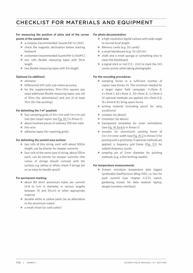
108 | GLORIA FIELD MANUAL – 5TH  EDITIONANNEX I

CHECKLIST FOR MATERIALS AND EQUIPMENT

For measuring the position of plots and of the corner points of the summit area

u a compass (recommended: Suunto KB-14/360)u check the magnetic declination before starting fieldworku a clinometer (recommended: Suunto PM-5/360PC)u two rolls flexible measuring tapes with 50 m lengthu two flexible measuring tapes with 3 m length

Optional (in addition):u altimeteru Differential GPS with sub-metre accuracyu for the supplementary 10 m × 10 m squares you need additional flexible measuring tapes: one roll of 50 m (for delimitation) and one of at least 10 m (for line-pointing)

For delimiting the 1-m² quadratsu four sampling grids of 3 m × 3 m with 1 m × 1 m cell size (per target region; see Fig. AI.1 in Annex I).u about hundred pieces of ordinary 100 mm nailsu thin wireu adhesive tapes (for repairing grids)

For delimiting the summit area sectionsu two rolls of thin string, each with about 500 m length; can be shorter for steeper summitsu four rolls of the same type of string, about 100 m each; can be shorter for steeper summits (the colour of strings should contrast with the surface; e.g. yellow or white; check if strings are on an easy-to-handle spool)

For permanent markingu about 80 short aluminium tubes per summit (0.8 to 1 cm in diameter, in various lengths between 10 and 25 cm) or other appropriate materialu durable white or yellow paint (as an alternative to the aluminium tubes)u a small chisel (or cold cutter)

For photo documentationu a high-resolution digital camera with wide-angle to normal focal lengthu Memory cards (e.g. SD cards)u a small blackboard (e.g. 15 × 20 cm)u chalk and a small sponge or something else to clean the blackboardu a signal stick or rod (1.5 - 2 m) to mark the SAS corner points while taking photographs

For the recording proceduresu sampling forms in a sufficient number of copies (see Annex II). The minimum needed for a target region field campaign: 1 × Form 0, 4 × Form  1, 64 × Form 2, 32 × Form 3, 4 × Form  4 (if optional methods are applied: 64 × Form 5-S, 16 × Form 6-S); bring spare forms.u writing material (including pencil for rainy conditions)u compass (as above)u clinometer (as above)u transparent templates for cover estimations (see Fig. AI.3a & b in Annex I)u wooden (or aluminium) pointing frame of 1 m × 1 m inner width (see Fig. AI.2 in Annex I) for pointing with a grid frame; if optional methods are applied: a frequency grid frame (Fig. 5.1) for subplot-frequency countsu sampling pin of 2 mm diameter for pointing methods (e.g. a thin knitting needle)

For temperature measurementsu Sixteen miniature temperature data loggers (preferably GeoPrecision Mlog-5W), i.e. four for each summit (see chapter 4.3.2), watch, gardening trowel, for data readout: laptop, dongle (wireless interface).

ANNEX I | 109GLORIA FIELD MANUAL – 5TH  EDITION

Tape

s ju

t out

for 0

.5 m

on

each

sid

efo

r fixi

ng th

e gr

id in

fiel

d

Star

t of t

heta

pe ro

ll

16 c

ross

ings

at t

he

met

re m

arks

, fixe

dto

geth

er w

ith m

etal

eyel

ets

Qua

drat

siz

e =

1 m fr

om e

yele

t to

eyel

et

Smal

l met

al e

yele

t (0

.4 c

m in

ner d

iam

eter

) fix

ing

two

tape

s to

geth

er

Fig. AI.1 Construction of the 3 m× 3 m grids.

Ste

p 1

. Pre

par

atio

n o

f 8

pie

ces

of

flex

ible

mea

suri

ng

tap

es o

f 4

 m le

ng

th: T

hes

e p

iece

s ar

e cu

t o

ff f

rom

e.g

. a 5

0-m

tap

e m

easu

re r

oll

(th

e fi

rst

at t

he

3.5

 m m

ark,

th

e se

con

d a

t th

e 7.

5 m

mar

k, a

nd

so

on

).

Ste

p 2

. At

each

met

re m

ark

of

all 8

tap

es, a

ro

un

d h

ole

of

0.4

 cm

dia

met

er is

pu

nch

ed in

th

e m

idd

le o

f th

e ta

pe

(= 4

ho

les

per

tap

e).

Ste

p 3

. Th

e 8

tap

es a

re a

rran

ged

into

a 3

 m  ×

  3  m

gri

d: c

olu

mn

tap

es a

nd

ro

w t

apes

are

fi

xed

to

get

her

wit

h s

mal

l met

al b

lan

ks (

i. e.

eye

lets

of

0.4

 cm

dia

met

er).

Eye

lets

are

pu

t th

rou

gh

th

e 2

ho

les

at e

ach

cro

ssin

g p

oin

t an

d r

ivet

ed w

ith

sp

ecia

l plie

rs

wh

ich

are

usu

ally

so

ld w

ith

th

e ey

elet

s.T

he

resu

lt is

a 3

 m  ×

  3  m

gri

d w

ith

1 m

  ×  1

  m s

ub

div

isio

ns.

No

te t

hat

eac

h s

ub

div

isio

n is

slig

htl

y sm

alle

r th

an 1

 m²,

bec

ause

of

the

wid

th o

f th

e ta

pe.

Th

is m

ino

r re

du

ctio

n o

fea

ch q

uad

rat

area

is a

ccep

ted

bec

ause

of

two

ad

van

tag

es:

(1)

the

con

stru

ctio

n o

f th

e ta

pe

is le

ss c

om

plic

ated

bec

ause

th

e in

ner

wid

th o

f th

e q

uad

rat

nee

d n

ot

be

mea

sure

d b

efo

re p

un

chin

g t

he

ho

les;

(2

) th

e sc

ale

at t

he

del

imit

atio

ns

of

the

sam

plin

g q

uad

rat

ran

ges

exa

ctly

fro

m o

ne

to

the

nex

t m

etre

mar

k -

this

is h

elp

ful f

or

cove

r es

tim

atio

n. E

ach

tap

e ju

ts o

ut

fro

m t

he

3 ×

 3 m

gri

d a

rea

for

0.5

 m o

n e

ach

sid

e. T

his

is h

elp

ful f

or

fixi

ng

th

e g

rid

in t

he

fiel

d.

Fo

ur

such

gri

ds

are

to b

e co

nst

ruct

ed (

on

e fo

r ea

ch 3

 m ×

 3 m

plo

t cl

ust

er).

Gri

ds

are

to b

e re

mo

ved

aft

er fi

eld

wo

rk a

t a

sum

mit

sit

e is

fin

alis

ed.

Th

eref

ore

, on

e se

t o

f 4

gri

ds

is s

uffi

cien

t fo

r o

ne

targ

et r

egio

n.

110 | GLORIA FIELD MANUAL – 5TH  EDITIONANNEX I

Fig.AI.2.

Step 1. Construction of 4 equal pieces of small wooden slats (3 cm × 1.5 cm and 106 cm length):

3 × 3 cm overlap area with a 0.6 to 0.7 cmdrill-hole in its centre

3 × 3 cm overlap area with a 0.6 to 0.7 cmdrill-hole in its centre

Ten narrow (0.3 cm) drill holes in 10 cm intervals (and 5 cm from the margins)

Step 2. Fixing the 4 pieces together:

Step 3. Threading and tightening of the strings:

Start with a knot (knot should be here at the bottom side)

a) String for the columns is alignedat the upper side of the wooden slats

b) String for the rows is aligned at the bottom side of the wooden slats, interwoven with the column string

Broken lines indicate string position on the bottom side

End with a knotafter tightening

The four pieces fixedtogether with screws and wing nuts

(the 2 horizontal slats are mounted below the 2 vertical slats)

3 × 3cmoverlap areas

3 × 1.5 cm

Screw of 4.5 cm lengthand 0.5 cm thread-diameter

Wing nut

Qua

dra

t si

ze: 1

m

Fig. AI.2 Construction of the 1 m× 1 m grid frame for pointing with 100 crosshair points.

ANNEX I | 111GLORIA FIELD MANUAL – 5TH  EDITION

170mm

.01

1

.8

.9

.6

.7

.5

.4

.3

.2

.15

.25

.1

.075

.025

.05

.005

.75

100m

m

Rectangular shapes ITemplates for percentage estimationsNumbers indicate % values of a 1m x 1m quadrat

GLORIA 2001

Rectangular shapes IITemplates for percentageestimationsNumbers indicate % valuesof a 1m x 1m quadrat

GLORIA 2001

1

.8

.9

.6

.7

.5

.4

.3

.2

.15

.25

.1.075

.025

.05

.01.005

.75

79m

m

170mm

1

.8.9

.6.7

.5

.4

.3

.2.15

.25

.1.075

.025.05

.01.005

.75

59m

m

Rectangular shapes III - Templates for percentage estimations - Numbers indicate % values of a 1m x 1m quadrat

GLORIA 2001

170mm

Fig. AI.3a.

Fig. AI.3a Templates for percentage cover estimations: rectangular shapes. These templates may be copied to a transparency and prepared for the field work. Make sure that the original size is maintained (i.e. when photocopying).

112 | GLORIA FIELD MANUAL – 5TH  EDITIONANNEX I

170mm

1.8 .9.6 .7.5.4.3.2.15 .25.1.075.025 .05.01.005 .75

100m

m

Elliptic shapes - Templates for percentage estimations - Numbers indicate % values of a 1m x 1m quadrat GLORIA 2001

1.8 .9.6 .7.5.4.3.2.15 .25.1.075.025 .05.01.005 .75

170mm

125m

m

Circular shapesTemplates for percentageestimationsNumbers indicate % valuesof a 1m x 1m quadrat

GLORIA 2001

Fig. AI.3b.

Fig. AI.3b Templates for percentage cover estimations: circular and elliptic shapes. These templates may be copied to a transparency and prepared for the field work. Make sure that the original size is maintained (i.e. when photocopying).

| 113GLORIA FIELD MANUAL – 5TH  EDITIONANNEX II

THE GLORIA FIELD MANUAL

ANNEX II: DATA SAMPLING FORMS

PART 1: SAMPLING FORMS

STANDARD SAMPLING FORMSForm 0 Target region  114Form 1 Measurement protocol  115Form 2 1-m² quadrat (with notes on a separate page*)  116Form 3 Summit area section (with notes on a separate page*)  118Form 4 Temperature loggers  120

SUPPLEMENTARY SAMPLING FORMSForm 5-S Subplot-frequency counts in the 1-m² quadrat  121Form 6-S 10 m × 10 m square (with notes on a separate page*)  122

* For fieldwork, notes should be printed on the backside of the form.

114 | GLORIA FIELD MANUAL – 5TH  EDITIONANNEX II

Form

0

Targ

et re

gion

Com

men

ts o

n ve

geta

tion

boun

dary

line

s3)

Cou

ntry

cod

e1)D

ate

Res

earc

her(s

)Ta

rget

regi

on c

ode1)

Alti

tude

of m

ajor

veg

etat

ion

boun

dary

line

s (in

met

res)

Pote

ntia

l nat

ural

fore

stlin

e2)Po

tent

ial n

atur

al tr

eelin

e2)Al

pine

-niv

al e

coto

ne2)

Cur

rent

fore

stlin

e2)C

urre

nt tr

eelin

e2)

SUM

MIT

SSu

mm

it co

de1)

Altit

ude

(m a

.s.l.

)

LOW

HIG

H

Use

ext

ra b

lank

she

ets,

if n

eces

sary

- in

dica

te th

e nu

mbe

r of e

xtra

she

ets

in th

is b

ox (e

.g. 1

of 2

, 2 o

f 2 e

tc…

)

Pred

omin

ant b

edro

ck m

ater

ial

and

appr

oxim

ate

soil

pH a

t the

su

mm

it si

tes

of th

e ta

rget

re

gion

4)

Shor

t des

crip

tion

of th

e ta

rget

regi

on, p

artic

ular

ly re

gard

ing

land

use

his

tory

and

the

curre

nt la

nd u

se s

ituat

ion

5)

Com

men

ts o

n th

e su

mm

it si

tuat

ion7)

Vege

tatio

n zo

neor

eco

tone

6)Su

mm

it na

me

Note

s

1)Se

e Bo

x 6.

1 fo

r cod

ing.

2)

Ente

r the

app

roxi

mat

ive

met

res

abov

e se

a le

vel (

m a

.s.l.

) for

eac

h ve

geta

tion

boun

dary

line

whi

ch in

dica

tes

its a

vera

ge a

ltitu

de in

the

targ

et re

gion

;the

fore

stlin

e (o

r tim

berli

ne) i

s de

fined

as

the

line

whe

re c

lose

d fo

rest

s en

d; th

e tre

elin

e is

def

ined

as

the

line

whe

re g

roup

s of

tree

s ta

ller t

han

3m e

nd; t

he a

lpin

e-ni

val e

coto

ne is

the

trans

ition

zon

e be

twee

n th

e up

per a

lpin

e be

lt an

d th

e ni

val b

elt -

mak

e an

est

imat

ion

of th

e al

titud

e of

the

uppe

r bou

ndar

y lin

e of

the

alpi

ne z

one,

whe

re c

lose

d ve

geta

tion

ends

(thi

s lin

e m

ay c

oinc

ide

with

the

perm

afro

st

limit

in m

any

mou

ntai

n re

gion

s).

3)W

here

requ

ired

mak

e co

mm

ents

on

the

indi

cate

d al

titud

inal

pos

ition

s of

bou

ndar

y lin

es; e

.g. d

evia

tions

from

the

aver

age

altit

ude;

men

tion

if a

boun

dary

line

do

es n

ot e

xist

in th

e ta

rget

regi

onan

d co

mm

ent o

n th

e re

ason

s fo

r its

abs

ence

. 4

)Bed

rock

mat

eria

l of t

he s

umm

it si

tes

of th

e ta

rget

regi

on, w

hich

sho

uld

be c

onsi

sten

t thr

ough

out t

he fo

ur

sum

mits

(con

sist

ent r

egar

ding

the

influ

ence

of t

he b

edro

ck o

n th

e sp

ecie

s co

mpo

sitio

n); i

n ad

ditio

n, m

ake

a ro

ugh

estim

ate

onth

e av

erag

e so

il pH

(e.g

. aci

d: <

4.5,

inte

rmed

iate

: 4.5

-6.5

, ne

utra

l/alk

alin

e: >

6.5)

. 5

)If t

he s

ituat

ion

is n

ot p

ristin

e or

nat

ural

, ind

icat

e w

hat k

ind

of la

nd u

se h

ave

or h

ad a

n im

pact

on

the

pres

ent v

eget

atio

n.

6)O

nly

the

follo

win

g en

tries

are

pos

sibl

e:

treel

ine

ecot

one,

low

er a

lpin

e, lo

wer

/upp

er a

lpin

e ec

oton

e, u

pper

alp

ine,

alp

ine-

niva

l eco

tone

, niv

al.

7)M

ake

com

men

ts o

n th

e si

tuat

ion

of th

e pa

rticu

lar s

umm

it if

vege

tatio

n zo

ne o

r eco

tone

is

not p

rope

rly a

pplic

able

and

des

crib

e th

e de

viat

ions

. Fur

ther

com

men

t on

any

othe

r pro

noun

ced

devi

atio

n fro

m a

n ‘id

eal’

stan

dard

sum

mit

situ

atio

n (c

ompa

re c

hapt

er 2

.2 in

the

field

man

ual).

Altitude

| 115GLORIA FIELD MANUAL – 5TH  EDITIONANNEX II

Form

1

Mea

sure

men

t pro

toco

lC

ount

ry c

ode1)

Dat

eG

eogr

aphi

c co

-ord

inat

es (d

eg/m

in/s

ec)

Targ

et re

gion

cod

e1)R

esea

rche

r(s)

long

.

Sum

mit

code

1)la

t.

Sum

mit

nam

e2)M

agne

tic d

eclin

atio

n (°

) for

com

pass

mea

sure

men

ts4)

QU

AD

RA

T C

LUST

ERS

& 1

0-m

PO

INTS

INTE

RSE

CTI

ON

LIN

ES

Dis

tanc

e (m

)6)Po

int n

um.

Com

p.

dir.

(°)7)

Phot

o ch

eck8)

Poin

t num

. Dis

t. (m

)6)C

omp.

di

r. (°

)7)Ph

oto

chec

k8)

p5m

-N11

q

uadr

at N

11pN

E-5

pSW

-5

p5m

-N31

q

uadr

at N

31pN

E-10

pSW

-10

p-N

33

qua

drat

N33

pSE-

5pN

W-5

p-N

13

qua

drat

N13

pSE-

10pN

W-1

0

p10m

-N

1

0-m

-poi

nt

p5m

-E11

q

uadr

at E

11C

OM

MEN

TSEn

tire

sum

mit

p5m

-E31

q

uadr

at E

31

Phot

o ch

eck8)

p-E3

3

qua

drat

E33

p-E1

3

qua

drat

E13

p10m

-E

1

0-m

-poi

nt

p5m

-S11

q

uadr

at S

11

p5m

-S31

q

uadr

at S

31

p-S3

3

qua

drat

S33

p-S1

3

qua

drat

S13

Use

ext

ra b

lank

she

ets

for f

urth

er re

mar

ks, i

f nec

essa

ry.

p10m

-S

1

0-m

-poi

ntIn

dica

te th

e nu

mbe

r of e

xtra

she

ets

in th

is b

ox

p5m

-W11

q

uadr

at W

11

p5m

-W31

q

uadr

at W

31

p-W

33

qua

drat

W33

p-W

13

qua

drat

W13

p10m

-W

1

0-m

-poi

nt

3mx3m grid cluster overview

WEST

3mx3m grid cluster overview

Hig

hest

sum

mit

poin

t (H

SP)3)

Altit

ude

(m)

SOUTH

Com

pass

di

rect

ion

(°)7)

Phot

o ch

eck8)

Dis

t. (m

)6)

NORTH

3mx3m grid cluster overview

3mx3m grid cluster overview

Poin

t num

ber5)

EAST

Not

es1)

See

Box

6.1

for c

odin

g.

2) F

ull n

ame

of th

e su

mm

it (fr

om to

pogr

aphi

c m

aps

or a

wor

king

nam

e w

here

no

offic

ial

nam

e is

ava

ilabl

e).

3)T

he h

ighe

st s

umm

it po

int i

s th

e cu

lmin

atio

n po

int +

/-in

the

mid

dle

of th

e su

mm

it ar

ea (r

ocky

ou

tcro

ps w

hich

may

be

high

er b

ut a

re n

ot c

entre

d in

the

sum

mit

area

sho

uld

be ig

nore

d).

4)

The

angl

e (w

ith it

s co

rrect

sig

n) b

etw

een

the

dire

ctio

n of

the

geog

raph

ic N

orth

Pol

e an

d of

the

mag

netic

Nor

th P

ole

(e.g

. -6

for a

mag

netic

dec

linat

ion

of 6

°W; +

10 fo

r 10°

E; s

ee B

ox 3

.1).

5)M

ark

thos

e ch

eckb

ox w

here

the

resp

ectiv

e po

int l

ies

on th

e pr

inci

pal

mea

sure

men

t lin

e (e

.g.,

p5m

-N11

or p

5m-N

31, b

oth

are

not p

ossi

ble;

com

pare

Fig

. 3.2

).

6) T

he le

ngth

of a

stra

ight

sur

face

line

bet

wee

n th

e H

SP a

nd th

e m

easu

rem

ent p

oint

(in

met

res,

with

two

deci

mal

pl

aces

); ke

ep th

e m

easu

rem

ent t

ape

tight

ened

for a

ll di

stan

ce m

easu

rem

ents

(see

Box

3.3

). 7

)The

com

pass

dire

ctio

n fro

m th

e H

SP to

the

mea

sure

men

t poi

nt in

deg

rees

(360

°sca

le; s

ee B

ox 3

.1).

Plea

se n

ote:

alw

ays

writ

e th

e m

agne

tic

com

pass

dire

ctio

ns (i

.e. d

egre

es a

s in

dica

ted

on th

e co

mpa

ss).

8)

Pho

to c

heck

: che

ck th

e bo

x af

ter p

hoto

s ar

e ta

ken

to m

ake

sure

that

the

phot

o do

cum

enta

tion

is c

ompl

ete

(see

und

er

4.4

for d

etai

ls).

Phot

o ch

eck8

)

116 | GLORIA FIELD MANUAL – 5TH  EDITIONANNEX II

Form 2 1-m² quadrat

Top cover of surface types (%)4)

Pointing hits9) Total hits10)

Subtypes in % of the top cover type5)

Plant species cover (%)6)

cf.7) Total hits10)

1

2

3

4

5

6

7

8

9

10

11

12

13

14

15

16

17

18

19

20

21

22

23

24

25

See back page for footnotes

Cover sum8) If you have used extra sheets, indicate their number (e.g. 1 of 2, 2 of 2 etc…)Total number of vascular plant species

Bryophytes on scree

Species %-cover6) Pointing hits9)

Lichens on solid rock Bryophytes on solid rock

Lichens on scree

100% General comments on the quadrat

Lichens below vasc. pl. Bryoph. below vasc. pl.

Bare ground

Litter

Lichens on soil not covered by vascular plants

Bryophytes on soil not covered by vascular plants

Vascular plants

Solid rock

Scree

Summit code1) Researcher(s) Slope (°)3)

Quadrat code1)

Country code1) Date Aspect2)

Target region code1) Recording time from to

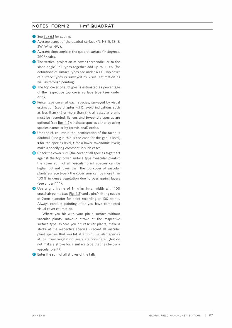
| 117GLORIA FIELD MANUAL – 5TH  EDITIONANNEX II

NOTES: FORM 2 1-m2 QUADRAT

1 See Box 6.1 for coding.2 Average aspect of the quadrat surface (N, NE, E, SE, S,

SW, W, or NW).3 Average slope angle of the quadrat surface (in degrees,

360° scale). 4 The vertical projection of cover (perpendicular to the

slope angle), all types together add up to 100% (for definitions of surface types see under 4.1.1). Top cover of surface types is surveyed by visual estimation as well as through pointing.

5 The top cover of subtypes is estimated as percentage of the respective top cover surface type (see under 4.1.1).

6 Percentage cover of each species, surveyed by visual estimation (see chapter 4.1.1); avoid indications such as less than (<) or more than (>); all vascular plants must be recorded; lichens and bryophyte species are optional (see Box 4.2); indicate species either by using species names or by (provisional) codes.

7 Use the cf. column if the identification of the taxon is doubtful (use g if this is the case for the genus level, s for the species level, t for a lower taxonomic level); make a specifying comment in such cases.

8 Check the cover sum (the cover of all species together) against the top cover surface type "vascular plants": the cover sum of all vascular plant species can be higher but not lower than the top cover of vascular plants surface type - the cover sum can be more than 100 % in dense vegetation due to overlapping layers (see under 4.1.1).

9 Use a grid frame of 1 m × 1 m inner width with 100 crosshair points (see Fig. 4.2) and a pin/knitting needle of 2 mm diameter for point recording at 100 points. Always conduct pointing after you have completed visual cover estimation.

Where you hit with your pin a surface without vascular plants, make a stroke at the respective surface type. Where you hit vascular plants, make a stroke at the respective species - record all vascular plant species that you hit at a point, i.e. also species at the lower vegetation layers are considered (but do not make a stroke for a surface type that lies below a vascular plant).

10 Enter the sum of all strokes of the tally.

118 | GLORIA FIELD MANUAL – 5TH  EDITIONANNEX II

Form 3 Summit area section (SAS)Codes of1) Top cover of surface types (%)2)

Country Researcher(s) Vascular plantsTarget region Solid rockSummit ScreeSAS Lichens (excl. epilithic)

BryophytesBare groundLitter

SUM 100%

Abun-dance6) cf.5)

Abun-dance6)

%-Cover7)

(optional)

1 31

2 32

3 33

4 34

5 35

6 36

7 37

8 38

9 39

10 40

11 41

12 42

13 43

14 44

15 45

16 46

17 47

18 48

19 49

20 50

21 51

22 52

23 53

24 54

25 55

26 56

27 57

28 58

29 59

30 60

Comments on species recording

See back page for footnotes

Comments on grazing impacts3)

Total number of vascular plant species in this summit area section

If you have used extrasheets, indicate their number (e.g. 1 of 3, 2 of 3, etc.)

Time from to

Species4) cf.5) %-Cover7)

(optional) Species4)

Date

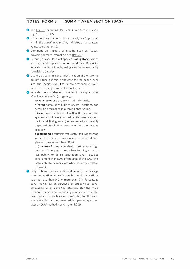
| 119GLORIA FIELD MANUAL – 5TH  EDITIONANNEX II

NOTES: FORM 3 SUMMIT AREA SECTION (SAS)

1 See Box 6.1 for coding; for summit area sections (SAS), e.g. N05, N10, E05.

2 Visual cover estimation of the surface types (top cover) within the summit area section, indicated as percentage value; see chapter 4.2.

3 Comment on impacts of grazing such as faeces, browsing damage, trampling; see Box 4.6.

4 Entering all vascular plant species is obligatory; lichens and bryophyte species are optional (see Box  4.2); indicate species either by using species names or by (provisional) codes.

5 Use the cf. column if the indentification of the taxon is doubtful (use g if this is the case for the genus level, s for the species level, t for a lower taxonomic level); make a specifying comment in such cases.

6 Indicate the abundance of species in five qualitative abundance categories (obligatory):

r! (very rare): one or a few small individuals.r (rare): some individuals at several locations, can hardly be overlooked in a careful observation.s (scattered): widespread within the section; the species cannot be overlooked but its presence is not obvious at first glance (not necessarily an evenly dispersed distribution over the entire summit area section).c (common): occurring frequently and widespread within the section – presence is obvious at first glance (cover is less than 50%).d (dominant): very abundant, making up a high portion of the phytomass, often forming more or less patchy or dense vegetation layers; species covers more than 50% of the area of the SAS (this is the only abundance class which is entirely related to cover).

7 Only optional (as an additional record): Percentage cover estimation for each species; avoid indications such as: less than (<) or more than (>). Percentage cover may either be surveyed by direct visual cover estimation or by point-line intercepts (for the more common species) and recording of area cover (i.e. the exact area size, such as m², dm², etc.; for the rarer species) which can be converted into percentage cover later on (PAF method; see chapter 5.2.2).

120 | GLORIA FIELD MANUAL – 5TH  EDITIONANNEX II

Form

4

Tem

pera

ture

logg

ers

C

ount

ry c

ode1)

Sum

mit

code

1)

Targ

et re

gion

cod

e1)Fu

ll su

mm

it na

me

Firs

t ins

talla

tion

Qua

drat

co

de1)

Logg

er s

eria

l2)Lo

gger

type

3)St

art d

ate

Star

t tim

e4)

(loca

l tim

e)U

TC

diff.

5)D

ist-1

16)D

ist-3

17)Ph

oto

chec

k op

en8)

Phot

o ch

eck

clos

ed8)

Res

earc

her(s

)C

omm

ents

□□

□□

□□

□□

Dat

a re

ad-o

ut D

e-in

stal

latio

n ne

eded

11)

Qua

drat

co

de1)

Logg

er s

eria

l2)Lo

gger

type

3)S

top

date

Sto

p tim

e9)

(loca

l tim

e)R

esea

rche

r(s)

Com

men

ts10

)N

ew

logg

er s

eria

l12)

Logg

er ty

pe3)

Star

t dat

eS

tart

time4)

(loca

l tim

e)

Pho

to

chec

k op

en8)

Pho

to

chec

k cl

osed

8)

□□

□□

□□

□□

1) S

ee B

ox 6

.1 fo

r cod

ing.

2)

The

logg

er s

eria

l num

ber i

s us

ually

indi

cate

d so

mew

here

on

the

logg

er a

nd is

the

refe

renc

e nu

mbe

r for

iden

tifyi

ng a

logg

er w

hen

laun

chin

g an

d re

adin

g ou

t the

dat

a.

3) In

dica

te th

e lo

gger

type

, e.g

. Geo

Prec

isio

n, T

idBi

t or T

inyT

ag.

4) In

dica

te th

e tim

e af

ter f

inis

hing

the

inst

alla

tion

of e

ach

logg

er in

the

field

(use

you

r loc

al ti

me)

. 5

) Ind

icat

e th

e tim

e di

ffere

nce,

i.e.

th

e nu

mbe

r of h

ours

to b

e ad

ded

or s

ubst

ract

ed fr

om y

our l

ocal

tim

e to

the

UTC

/GC

T (C

oord

inat

ed U

nive

rsal

Tim

e/G

reen

wic

h M

ean

Tim

e); f

or e

xam

ple,

if th

e lo

cal t

ime

is 1

4:00

and

UTC

12:

00, t

he

valu

e to

be

ente

red

is -2

. 6

) Dis

tanc

e (in

m w

ith tw

o de

cim

al p

lace

s) fr

om th

e lo

gger

to th

e le

ft lo

wer

clu

ster

cor

ner (

e.g.

p5m

-S11

; see

Fig

. 4.5

). 7

) Dis

tanc

e (in

m w

ith tw

o de

cim

al p

lace

s) fr

om th

e lo

gger

to th

e rig

ht lo

wer

clu

ster

cor

ner (

e.g.

p5m

-S31

; see

Fig

. 4.5

). 8

) Pho

to c

heck

: Che

ck th

e bo

x af

ter p

hoto

s ar

e ta

ken

to b

e su

re th

at th

e ph

oto

docu

men

tatio

n is

com

plet

e (d

ocum

enta

tion

of th

e lo

gger

pos

ition

with

the

hole

ope

n an

d do

cum

enta

tion

afte

r the

hol

e is

clo

sed

with

sub

stra

te m

ater

ial;

see

Fig.

4.5

). 9

) Ind

icat

e th

e tim

e of

dat

a re

ad-o

ut (u

se y

our l

ocal

tim

e). I

n ca

ses

whe

re d

e-in

stal

latio

n is

nec

cess

ary

indi

cate

the

time

befo

re d

iggi

ng o

ut th

e lo

gger

. 1

0)C

omm

ent o

n lo

gger

failu

re a

nd d

e-in

stal

latio

ns; i

n an

y ca

se w

hen

you

de-in

stal

l the

logg

er, i

ndic

ate

DR

for d

ata

read

-out

(e

.g. i

n th

e ca

se o

f Tid

Bit l

ogge

rs),

BC

for b

atte

ry c

hang

e, o

r LC

for l

ogge

r cha

nge.

11

)Onl

y to

be

fille

d ou

t whe

n yo

u de

-inst

all t

he lo

gger

. 1

2)In

dica

te th

e ne

w lo

gger

ser

ial n

umbe

r. In

cas

es o

f in

stal

ling

the

sam

e lo

gger

(bat

tery

cha

nge

or T

idBi

t dat

a re

ad-o

ut),

indi

cate

"ide

nt" f

or id

entic

logg

er.

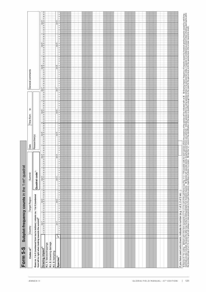
| 121GLORIA FIELD MANUAL – 5TH  EDITIONANNEX II

Form

5-S

S

ubpl

ot-fr

eque

ncy

coun

ts in

the

1-m

² qua

drat

Cod

es o

f1)

Cou

ntry

Targ

et R

egio

nSu

mm

itD

ate

Tim

e fro

m

to

G

ener

al c

omm

ents

Qua

drat

cod

e1)R

esea

rche

r(s)

12

34

56

78

90

12

34

56

78

90

12

34

56

78

90

12

34

56

78

90

12

34

56

78

90

12

34

56

78

90

12

34

56

78

90

12

34

56

78

90

12

34

56

78

90

12

34

56

78

90

H.i.

1: f

aece

s/dr

oppi

ngs

H.i.

2: b

row

sing

dam

age

H.i.

3: t

ram

plin

g

12

34

56

78

90

12

34

56

78

90

12

34

56

78

90

12

34

56

78

90

12

34

56

78

90

12

34

56

78

90

12

34

56

78

90

12

34

56

78

90

12

34

56

78

90

12

34

56

78

90

If yo

u ha

ve u

sed

extra

she

ets,

indi

cate

its

num

ber (

e.g.

1 o

f 2, 2

of 2

etc

…)

row

0ro

w 8

row

9

row

8ro

w 9

row

0ro

w 7

row

5ro

w 6

row

7

row

3ro

w 4

row

5ro

w 6

row

3ro

w 4

Spec

ies4)

cf.5)

row

1ro

w 2

Row

s no

. 1 to

0 (n

umbe

red

from

top

to b

otto

m);

colu

mn

no. 1

to 0

(num

bere

d fr

om le

ft to

righ

t whe

n lo

okin

g to

war

ds th

e su

mm

it)2)

Gra

zing

impa

ct3)

row

1ro

w 2

1)Se

e bo

x 6.

1 fo

r cod

ing.

2)

Each

cel

l in

this

form

repr

esen

ts a

0.1

m x

0.1

m c

ell o

f the

grid

fram

e (s

ee F

ig. 5

.1) =

100

pos

sibl

e ce

lls fo

r eac

h sp

ecie

s w

here

the

pres

ence

of t

he s

peci

es w

ill be

indi

cate

d w

ith a

n X.

3)

Gra

zing

impa

ct: f

requ

ency

of i

mpa

cts

caus

ed b

y liv

esto

ck g

razi

ng (i

mpa

cts

caus

ed b

y w

ild-li

ving

m

amm

als

are

also

incl

uded

, bec

ause

the

latte

r may

har

dly

be d

istin

guis

habl

e fro

m li

vest

ock

impa

cts)

. 4

)Spe

cies

(all

vasc

ular

pla

nts;

bry

ophy

tes

and

liche

ns a

re o

ptio

nal);

ind

icat

e sp

ecie

s ei

ther

by

usin

g sp

ecie

s na

mes

or b

y (p

rovi

sion

al) c

odes

. A s

peci

es is

con

side

red

as p

rese

nt w

hen

show

ing

plan

t par

ts w

ithin

th

e bo

unda

ry s

tring

s of

a 0

.1m

x 0

.1m

grid

cel

l (al

way

s in

vie

w p

erpe

ndic

ular

to th

e gr

id fr

ame

plan

e), r

egar

dles

s of

whe

re it

is ro

oted

. 5

) Use

the

"cf."

col

umn

if th

e id

entif

icat

ion

of th

e ta

xon

is d

oubt

ful (

use

gif

this

is th

e ca

se fo

r the

gen

us le

vel,

sfo

r the

spe

cies

leve

l,tf

or a

low

er ta

xono

mic

leve

l).

122 | GLORIA FIELD MANUAL – 5TH  EDITIONANNEX II

Form

6-S

10

m x

10m

squ

are

Cou

ntry

1)

Sum

mit1)

D

ate

Indi

cate

line

dire

ctio

n an

d po

sitio

n of

sta

rt lin

e3)

Res

earc

hers

TR

1)As

pect

2)Ti

me

from

to

Rec

ordi

ng L

ines

5)

Surf

ace

Type

s4)1

23

45

67

89

1011

1213

1415

1617

1819

20To

tal h

its6)

Solid

rock

Scre

e

Lich

ens

on s

oil

Bryo

phyt

es o

n so

il

Bare

gro

und

Litte

r

Spec

ies7)

12

34

56

78

910

1112

1314

1516

1718

1920

Tota

l hits

6)

Gen

eral

Com

men

ts

If yo

u ha

ve u

sed

extra

shee

ts, i

ndic

ate

thei

r num

ber (

e.g.

1 o

f 3, 2

of 3

, etc

.)

Mar

k on

e of

th

e fo

ur

optio

ns

| 123GLORIA FIELD MANUAL – 5TH  EDITIONANNEX II

NOTES: FORM 6-S GLORIA 10m ×  10m SQUARE

1 See Box 6.1 for coding.2 Enter the cardinal direction (N, E, S, or W).3 Indicate starting line position with a check mark at one

of the four options. 4 The same surface types as used in the summit area

sections, but without the surface type "vascular plants" (compare chapter 5.3.1). Surface types are only tallied where no vascular plants were hit.

5 Twenty parallel lines for line-pointing (column 1-20); twenty points along each line (compare chapter 5.3.1).

6 Enter the sum of all strokes of the tally.7 Enter all vascular plant species which you hit with the

sampling pin. When you hit more than one vascular plant species on one point, tally all of them. After you have completed line pointing, add (below or on a continuation sheet) all additional vascular plant species that occur within the 10 m × 10 m square.

124 | GLORIA FIELD MANUAL – 5TH  EDITIONANNEX II

THE GLORIA FIELD MANUAL

ANNEX II: DATA SAMPLING FORMS

PART 2: EXAMPLE SHEETS

Examples of standard sampling forms 0, 1-4  125 and of supplementary forms 5-S, 6-S  132

Example of the GLORIA target region Taxa input sheet  135

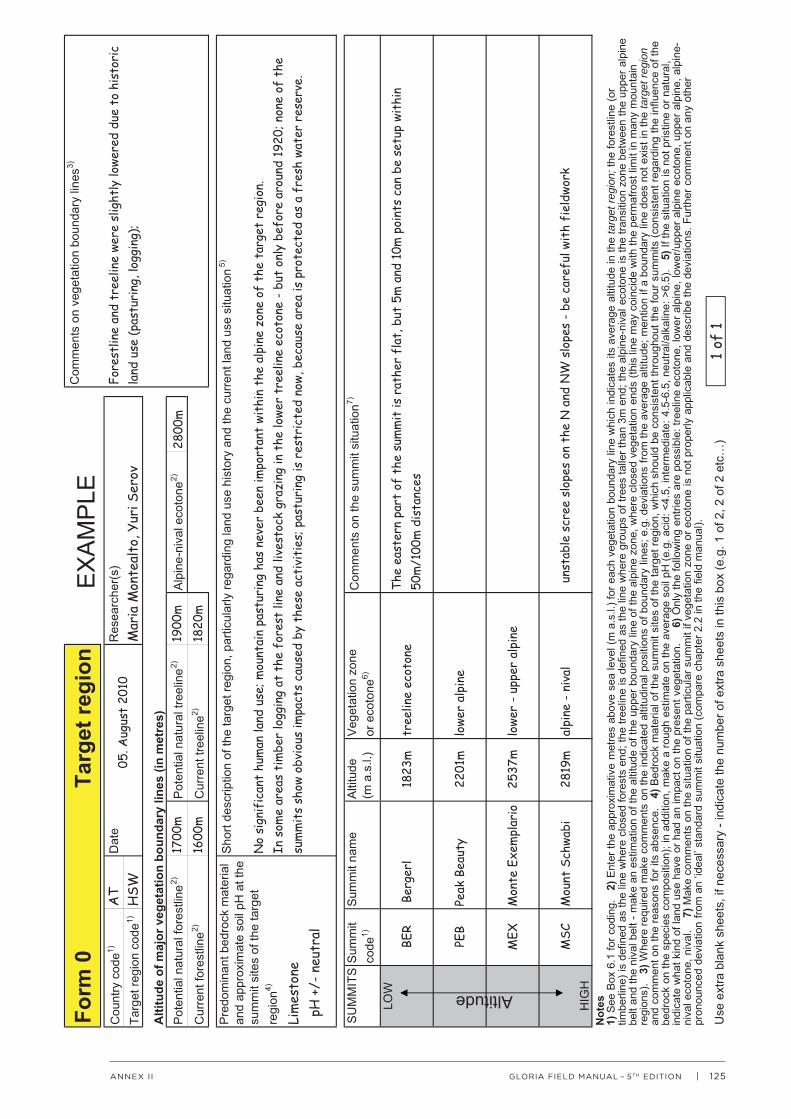
| 125GLORIA FIELD MANUAL – 5TH  EDITIONANNEX II

AT

HSW

Mar

ia M

onte

alto

, Yur

i Ser

ov

1700

m19

00m

2800

m16

00m

1820

m

BER

Berg

erl

1823

mtr

eelin

e ec

oton

e

PEB

Peak

Bea

uty

2201

mlo

wer

alpi

ne

MEX

Mon

te E

xem

plar

io25

37m

lowe

r -

uppe

r al

pine

MSC

Mou

nt S

chwa

bi28

19m

alpi

ne -

niv

al

Fore

stlin

e an

d tr

eelin

e we

re s

light

ly lo

were

d du

e to

his

tori

c la

nd u

se (p

astu

ring

, log

ging

);05

. Aug

ust

2010

The

east

ern

part

of

the

sum

mit

is r

athe

r fl

at, b

ut 5

m a

nd 1

0m p

oint

s ca

n be

set

up w

ithi

n 50

m/1

00m

dis

tanc

es

uns

tabl

e sc

ree

slop

es o

n th

e N

and

NW

slo

pes

- be

car

eful

wit

h fi

eldw

ork

Lim

esto

ne p

H +

/- n

eutr

al

No

sign

ific

ant

hum

an la

nd u

se; m

ount

ain

past

urin

g ha

s ne

ver

been

impo

rtan

t wi

thin

the

alp

ine

zone

of

the

targ

et r

egio

n.

In s

ome

area

s ti

mbe

r lo

ggin

g at

the

for

est

line

and

lives

tock

gra

zing

in t

he lo

wer

tree

line

ecot

one

- bu

t on

ly b

efor

e ar

ound

192

0; n

one

of t

he

sum

mit

s sh

ow o

bvio

us im

pact

s ca

used

by

thes

e ac

tivi

ties

; pas

turi

ng is

res

tric

ted

now,

bec

ause

are

a is

pro

tect

ed a

s a

fres

h wa

ter

rese

rve.

targ

et re

gion

;

targ

et re

gion

1 of

1

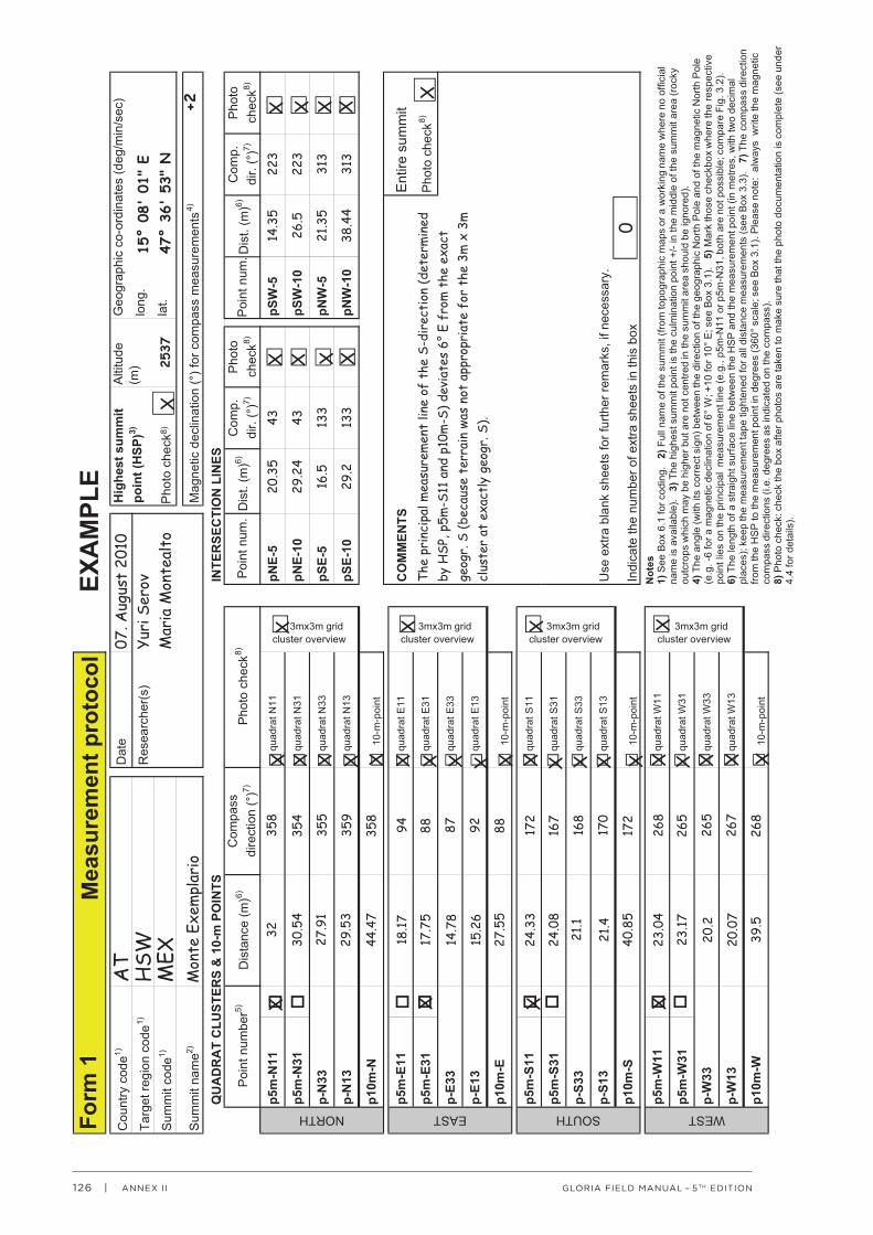
126 | GLORIA FIELD MANUAL – 5TH  EDITIONANNEX II

AT

07. A

ugus

t 20

10H

SWYu

ri S

erov

15°

08'

01"

EM

EXM

aria

Mon

teal

to47

° 36

' 53

" N

Mon

te E

xem

plar

io+2

3235

820

.35

4314

.35

223

30.5

435

429

.24

4326

.522

3

27.9

135

516

.513

321

.35

313

29.5

335

929

.213

338

.44

313

44.4

735

8

18.17

94

17.7

588

14.7

887

15.2

692

27.5

588

24.3

317

2

24.0

816

7

21.1

168

21.4

170

40.8

517

2

23.0

426

8

23.17

265

20.2

265

20.0

726

7

39.5

268

2537

The

prin

cipa

l mea

sure

men

t lin

e of

the

S-d

irec

tion

(det

erm

ined

by

HSP

, p5m

-S11

and

p10

m-S

) dev

iate

s 6°

E f

rom

the

exa

ct

geog

r. S

(bec

ause

ter

rain

was

not

app

ropr

iate

for

the

3m

x 3

m

clus

ter

at e

xact

ly g

eogr

. S).

0

X

XX

X

X

X X

X XX X X XXXX X X X X X XX XX

XXX X

X

X XXX

XXX

X

| 127GLORIA FIELD MANUAL – 5TH  EDITIONANNEX II

3982390

1.53520

215102

t 2

1

1

s

AT . August 2010 SEHSW 10:45 12:10MEX 17E31

8

3244

2.53100.5

20

Likely Festuca versic. ssp. brachy., but might also be F. quadriflora; Arabis: we think it is A. b. ssp. stellulata, but it also could be A. bellidifolia ssp. bellidifolia (for both cases see herbarium material collected outside the plot)

Carex firma 22

0

Festuca quadriflora 4Dryas octopetala 8Arenaria ciliata 1Arabis bellidifolia ssp. stellulata 0.5Carex fuliginosa 0.05Salix retusa 0.7Draba sauteri 0.001Salix reticulata 0.03Poa alpina 0.03Festuca versicolor subsp. brachystachys 1.2

1 of 111

37.5

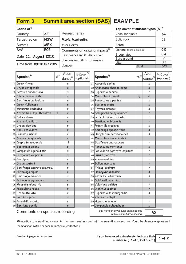
128 | GLORIA FIELD MANUAL – 5TH  EDITIONANNEX II

AT 64HSW Maria Montealto, 18MEX Yuri Serov 10E05 0.5

0.47

0.1

Carex firma c Agrostis alpina sDryas octopetala c Androsace chamaejasme sFestuca quadriflora s Euphrasia minima rSilene acaulis s.str. s Minuartia sp. small g r!Saxifraga paniculata r Ranunculus alpestris sCarex fuliginosa r Sesleria ovata sMinuartia sedoides r Thymus praecox sArabis bell. ssp. stellulata t r Selaginella selagionoides rSalix retusa r Pedicularis verticillata rArenaria ciliata r Gentiana orbicularis rDraba aizoides r Potentilla clusiana sSalix reticulata r Saxifraga oppositifolia sPrimula clusiana r Hedysarum hedysaroides sDoronicum glaciale r Minuartia cherlerioides rCrepis terglouensis r! Saxifraga androsacea rSesleria albicans s Ranunculus montanus sCampanula alpina s.str. s Pedicularis rostrato-capitata rPolygonum viviparum s Luzula glabrata rPoa alpina c Armeria alpina rDraba sauteri s Galium noricum rSaxifraga exarata ssp.mos. r Thlaspi alpinum rPritzelago alpina r Homogyne discolor sSaxifraga aizoides s Aster bellidiastrum sPetrocallis pyrenaica r Soldanella austriaca rMyosotis alpestris s Valeriana celtica rPedicularis rosea r Dianthus alpinus rDraba stellata r Euphrasia salisburgensis sBartsia alpina s Veronica aphylla rPotentilla crantzii s Huperzia selago rGentiana pumila r Campanula scheuchzeri s

1 of 2

Few faeces most likely from chamois and slight browsing damage

Minuartia sp.: a small individuum in the lower eastern part of the summit area section. Could be Arenaria sp. as well (comparison with herbarium material collected).

summit area section

09:30 12:05

11. August 2010

62

| 129GLORIA FIELD MANUAL – 5TH  EDITIONANNEX II

ATHSW Maria Montealto,MEX Yuri SerovE05

Festuca vers. ssp. brachyst. s rParnassia palustris r

summit area section

Festuca versic. ssp. brachy.: likely it is F. versic. ssp. brachy., but it could be F. quadriflora as well.

2 of 2

11. August 2010

09:30 12:05

62

continued

130 | GLORIA FIELD MANUAL – 5TH  EDITIONANNEX II

AT

MEX

HSW

Mon

te E

xem

plar

io

N22

A43

702

GeoP

reci

sion

12. A

ugus

t 20

1013

:05

+ 2

1.76

2.07

Mon

teal

to, S

erov

E22

A55

632

GeoP

reci

sion

12. A

ugus

t 20

1014

:30

+ 2

2.05

2.67

Mon

teal

to, S

erov

S22

A87

354

GeoP

reci

sion

12. A

ugus

t 20

1015

:21

+ 2

1.80

1.20

Mon

teal

to, S

erov

W22

A22

154

GeoP

reci

sion

12. A

ugus

t 20

1017

:15

+ 2

2.08

2.04

Mon

teal

to, S

erov

XX X

X

XXX

X

| 131GLORIA FIELD MANUAL – 5TH  EDITIONANNEX II

AT

MEX

HSW

Mon

te E

xem

plar

io

N22

A43

702

GeoP

reci

sion

12. A

ugus

t 20

1013

:05

+ 2

1.76

2.07

Mon

teal

to, S

erov

E22

A55

632

GeoP

reci

sion

12. A

ugus

t 20

1014

:30

+ 2

2.05

2.67

Mon

teal

to, S

erov

S22

A87

354

GeoP

reci

sion

12. A

ugus

t 20

1015

:21

+ 2

1.80

1.20

Mon

teal

to, S

erov

W22

A22

154

GeoP

reci

sion

12. A

ugus

t 20

1017

:15

+ 2

2.08

2.04

Mon

teal

to, S

erov

N22

A43

702

GeoP

reci

sion

03. A

ugus

t 20

1311

:25

Mon

teal

to,

Sero

vBC

iden

t03

. Aug

ust

2013

12:0

5

E22

A55

632

GeoP

reci

sion

03. A

ugus

t 20

1312

:33

Mon

teal

to,

Sero

vLC

no s

i gna

l fro

m t

he lo

gger

A23

234

GeoP

reci

sion

03. A

ugus

t 20

1312

:59

S22

A87

354

GeoP

reci

sion

03. A

ugus

t 20

1313

:19

Mon

teal

to,

Sero

vBC

iden

t03

. Aug

ust

2013

13:5

0

W22

A22

154

GeoP

reci

sion

03. A

ugus

t 20

1314

:45

Mon

teal

to,

Sero

vBC

iden

t03

. Aug

ust

2013

15:1

0

XX

XX

XX

XX

XX X

X X

XX

X

132 | GLORIA FIELD MANUAL – 5TH  EDITIONANNEX II

Form

5-S

Subp

lot-f

requ

ency

cou

nts

in th

e 1-

m² q

uadr

atEX

AMPL

EC

odes

of1)

C

ount

ryA

TTa

rget

Reg

ion

HSW

Sum

mit

MEX

Dat

e13

. Aug

ust

2010

Tim

e fro

m 0

9:35

to11

:14

Gen

eral

com

men

ts

Qua

drat

cod

e1)E3

1R

esea

rche

r(s)

Mon

teal

to, S

erov

12

34

56

78

90

12

34

56

78

90

12

34

56

78

90

12

34

56

78

90

12

34

56

78

90

12

34

56

78

90

12

34

56

78

90

12

34

56

78

90

12

34

56

78

90

12

34

56

78

90

H.i.

1: f

aece

s/dr

oppi

ngs

H.i.

2: b

row

sing

dam

age

H.i.

3: t

ram

plin

g

12

34

56

78

90

12

34

56

78

90

12

34

56

78

90

12

34

56

78

90

12

34

56

78

90

12

34

56

78

90

12

34

56

78

90

12

34

56

78

90

12

34

56

78

90

12

34

56

78

90

Care

x fi

rma

Fest

uca

quad

rifl

ora

Dry

as o

ctop

etal

a

Are

nari

a ci

liata

Ara

bis

belli

difo

lia s

sp. s

tellu

lata

t

Care

x fu

ligin

osa

Salix

ret

usa

Dra

ba s

aute

ri

Salix

ret

icul

ata

Poa

alpi

na

Fest

uca

vers

icol

or s

sp. b

rach

ysta

chys

s

If yo

u ha

ve u

sed

extra

she

ets,

indi

cate

its

num

ber (

e.g.

1 o

f 2, 2

of 2

etc

…)

row

4ro

w 0

row

8ro

w 9

row

8ro

w 9

row

0ro

w 5

row

6ro

w 7

row

5ro

w 6

row

7

Row

s no

. 1 to

0 (n

umbe

red

from

top

to b

otto

m);

colu

mn

no. 1

to 0

(n

umbe

red

from

left

to ri

ght w

hen

look

ing

tow

ards

the

sum

mit)

2)

Gra

zing

impa

ct3)

row

1ro

w 2

row

4

row

3

row

3

Spec

ies4)

cf.5)

row

1ro

w 2

1 of

1

1)Se

e bo

x 6.

1 fo

r cod

ing.

2)

Each

cel

l in

this

form

repr

esen

ts a

0.1

m x

0.1

m c

ell o

f the

grid

fram

e (s

ee F

ig. 5

.1) =

100

pos

sibl

e ce

lls fo

r eac

h sp

ecie

s w

here

the

pres

ence

of t

he s

peci

es w

ill be

indi

cate

d w

ith a

n X.

3)

Gra

zing

impa

ct: f

requ

ency

of i

mpa

cts

caus

ed b

y liv

esto

ck g

razi

ng (i

mpa

cts

caus

ed b

y w

ild-

livin

g m

amm

als

are

also

incl

uded

, bec

ause

the

latte

r may

har

dly

be d

istin

guis

habl

e fro

m li

vest

ock

impa

cts)

. 4

)Spe

cies

(all

vasc

ular

pla

nts;

bry

ophy

tes

and

liche

ns a

re o

ptio

nal);

ind

icat

e sp

ecie

s ei

ther

by

usin

g sp

ecie

s na

mes

or b

y (p

rovi

sion

al) c

odes

. A s

peci

es is

con

side

red

as p

rese

nt w

hen

show

ing

plan

t pa

rts w

ithin

the

boun

dary

stri

ngs

of a

0.1

x 0

.1m

grid

cel

l (al

way

s in

vie

w p

erpe

ndic

ular

to th

e gr

id fr

ame

plan

e), r

egar

dles

s of

whe

re it

is ro

oted

. 5

) Use

the

"cf."

col

umn

if th

e id

entif

icat

ion

of th

e ta

xon

is d

oubt

ful (

use

gif

this

is th

e ca

se fo

r the

gen

us le

vel,

sfo

r the

spe

cies

leve

l,tf

or a

low

er ta

xono

mic

leve

l).

45

64

65

45

23

544

56

56

| 133GLORIA FIELD MANUAL – 5TH  EDITIONANNEX II

Form

6-S

10

m x

10m

squ

are

Cou

ntry

1) AT

Sum

mit1)

M

EXD

ate

14.

Aug

ust

2010

Indi

cate

line

dire

ctio

n an

d po

sitio

n of

sta

rt lin

e3)

Res

earc

hers

Mar

ia M

onte

alto

, Se

rov

TR1)

HSW

Asp

ect2)

E

Tim

e fro

m 1

0:00

to 1

2:20

Rec

ordi

ng L

ines

5)

Surf

ace

Type

s4)1

23

45

67

89

1011

1213

1415

1617

1819

20To

tal h

its6)

Sol

id ro

ck13

9

Scr

ee52

Lich

ens

on s

oil

1

Bry

ophy

tes

on s

oil

2

Bar

e gr

ound

5

Litte

r0

Spec

ies7)

12

34

56

78

910

1112

1314

1516

1718

1920

Tota

l hits

6)

Care

x fi

rma

101

Dry

as o

ctop

etal

a24

Poa

alpi

na21

Fest

uca

quad

rifl

ora

12Si

lene

aca

ulis

s.s

tr.

19Ca

mpa

nula

alp

ina

s.st

r.6

Agr

osti

s al

pina

8Po

lygo

num

viv

ipar

um3

Saxi

frag

a ai

zoid

es1

Myo

soti

s al

pest

ris

3Pr

imul

a cl

usia

na2

Pote

ntill

a cr

antz

ii3

Sesl

eria

alb

ican

s5

Salix

ret

usa

1D

raba

sau

teri

1Sa

xifr

aga

ex. s

sp. m

os.

1Ca

mpa

nula

sch

euch

zeri

3Ra

nunc

ulus

alp

estr

is1

And

rosa

ce c

ham

aeja

s.1

Euph

rasi

a sa

lisbu

rgen

.2

Saxi

frag

a an

dros

ace

1Ra

nunc

ulus

mon

tanu

s1

Ast

er b

ellid

iast

rum

1

Vale

rian

a ce

ltic

a

Gen

eral

Com

men

ts

If yo

u ha

ve u

sed

extra

shee

ts, i

ndic

ate

thei

r num

ber (

e.g.

1 o

f 3, 2

of 3

, etc

.)

Mar

k on

e of

th

e fo

ur

optio

ns

Spec

ies

with

no

hits

:

1 of

2

��

EXAM

PLE

134 | GLORIA FIELD MANUAL – 5TH  EDITIONANNEX II

Form

6-S

10

m x

10m

squ

are

Cou

ntry

1) A

TS

umm

it1) M

EXD

ate

14. Aug

ust

2010

Indi

cate

line

dire

ctio

n an

d po

sitio

n of

sta

rt lin

e3)

Res

earc

hers

Mar

ia M

onte

alto

, Se

rov

TR1)

HSW

Asp

ect2)

ETi

me

from

10:

00 to

12:

20

Rec

ordi

ng L

ines

5)

Surf

ace

Type

s4)1

23

45

67

89

1011

1213

1415

1617

1819

20To

tal h

its6)

Sol

id ro

ck

Scr

ee

Lich

ens

on s

oil

Bry

ophy

tes

on s

oil

Bar

e gr

ound

Litte

r

Spec

ies7)

12

34

56

78

910

1112

1314

1516

1718

1920

Tota

l hits

6)

Arm

eria

alp

ina

Saxi

frag

a op

posi

tifo

l.H

uper

zia

sela

goGe

ntia

na o

rbic

ular

isH

edys

arum

hed

ysar

.Pe

dicu

lari

s ve

rtic

illat

aSe

sler

ia o

vata

Gen

eral

Com

men

ts

If yo

u ha

ve u

sed

extra

shee

ts, i

ndic

ate

thei

r num

ber (

e.g.

1 o

f 3, 2

of 3

, etc

.)

Mar

k on

e of

th

e fo

ur

optio

ns

2 of

2

��

EXAM

PLE co

ntinu

ed

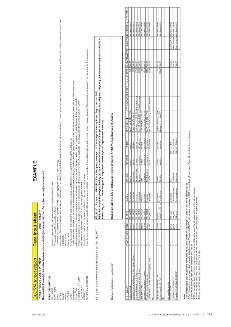
| 135GLORIA FIELD MANUAL – 5TH  EDITIONANNEX II

GLO

RIA

targ

et re

gion

136 | GLORIA FIELD MANUAL – 5TH  EDITIONANNEX III

Any item which is included into the GLORIA photo documentation must have a GLORIA-wide unique code. This code has to be indicated on the blackboard included in the photo view, wherever applicable. Moreover, digital photos which are to be sent to the Central GLORIA Database must have their filenames coded accordingly.

The software for maintaining your digital photo documentation (GPDM, GLORIA Photo Data Management) as provided by the GLORIA coordination is designed to compose these filenames automatically for you in order to prevent typing errors as far as possible. Moreover, it is the basis for including your photos in the logical structure of the Central GLORIA Database and of the GLORIA website. Therefore, it is highly recommended that you use this software. You can download this software from the GLORIA website (www.gloria.ac.at), please also see the explanations included in the software package on how to use it.

FORMAT AND SIZE OF THE PHOTO FILEOnly JPEG files (*.jpg) are accepted for the Central GLORIA Database and website. Use high pixel resolution and do not use a high JPEG-compression factor of your digital photos. Keep in mind that with low resolutions and high compressions you may lose some valuable visual information of the photo. Pictures should have at least about 2000 × 1500 pixels with a JPEG compression of not more than 20 (on a compression scale of 2 to 255, high quality to low quality). The resulting files should have a size of at least 1.5 MB. Higher resolutions and file sizes, of up to about 5-7 MB, are accepted and may be preferable, but do not use TIFF or RAW IMAGE formats.

STRUCTURE OF PICTURE CODINGThe codes are composed of several elements. These elements are defined below. Some of them are required, while others are not. Likewise, some elements have a fixed character length, others do not, due to already established coding conventions according to this manual (compare Fig. 3.2 and Box 6.1).

NAMES OF DIGITAL PHOTO FILESIt should be possible to sort all digital photo files logically by their filenames. Therefore, any element must have a constant length in the filenames. If a code is shorter than the required element length, one or more underscores ( _ ) have to be appended. The code elements themselves also have to be separated by underscores in the filename (and not blanks or dots or hyphens, as opposed to the writing on the blackboard).

In many cases, more than one photo exists for the same item. Therefore, the rightmost fixed-length code element in the filename (i.e., element 7, see below) is defined as ordering number. Each photo file of your target region must have a unique ordering number. The software GPDM creates this automatically for you. If you want certain photos (of the same item) to appear in a certain order at the GLORIA website (e.g. because of decreasing importance or quality), reflect this order in the numbering of this code element.

THE GLORIA FIELD MANUALMULTI-SUMMIT APPROACH

ANNEX III: CODING OF THE PHOTO DOCUMENTATION

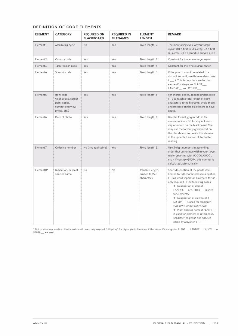
| 137GLORIA FIELD MANUAL – 5TH  EDITIONANNEX III

DEFINITION OF CODE ELEMENTS

ELEMENT CATEGORY REQUIRED ON BLACKBOARD

REQUIRED IN FILENAMES

ELEMENT LENGTH

REMARK

Element 1 Monitoring cycle No Yes Fixed length: 2 The monitoring cycle of your target region (01 = first field survey, 02 = first re-survey, 03 = second re-survey, etc.)

Element 2 Country code Yes Yes Fixed length: 2 Constant for the whole target region

Element 3 Target region code Yes Yes Fixed length: 3 Constant for the whole target region

Element 4 Summit code Yes Yes Fixed length: 3 If the photo cannot be related to a distinct summit, use three underscores ( ___ ). This is only the case for the element5-categories PLANT___, LANDSC__, and OTHER___.

Element 5 Item code (plot codes, corner point codes, summit overview photo, etc,)

Yes Yes Fixed length: 8 For shorter codes, append underscores ( _ ) to reach a total length of eight characters in the filename; avoid these underscores on the blackboard to save space.

Element 6 Date of photo Yes Yes Fixed length: 8 Use the format yyyymmdd in file names: indicate 00 for any unknown day or month on the blackboard. You may use the format yyyy/mm/dd on the blackboard and write this element in the upper left corner of, for better reading.

Element 7 Ordering number No (not applicable) Yes Fixed length: 5 Use 5-digit numbers in ascending order that are unique within your target region (starting with 00000, 00001, etc.); if you use GPDM, this number is calculated automatically.

Element 8* Indication, or plant species name

No No Variable length, limited to 150 characters

Short description of the photo item; limited to 150 characters; use a hyphen ( - ) as word separator. However, this is only required in the following cases:

u Description of item if LANDSC__, or OTHER___ is used for element5; u Description of viewpoint if SU-OV___ is used for element 5 (SU-OV: summit overview); u Plant species name if PLANT___ is used for element 5; in this case, separate the genus and species name by a hyphen ( - )

* Not required (optional) on blackboards in all cases; only required (obligatory) for digital photo filenames if the element 5- categories PLANT___, LANDSC___, SU-OV___ or OTHER___ are used