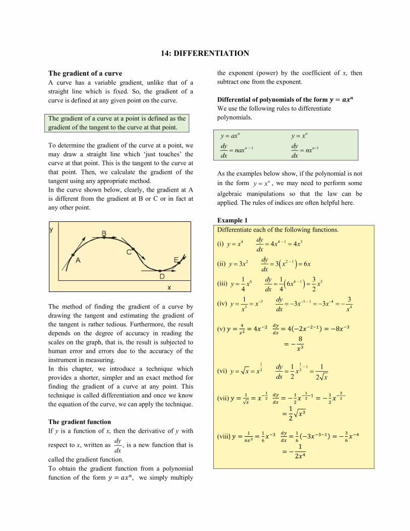
14: DIFFERENTIATION The gradient of a curve A curve has a variable gradient, unlike that of a straight line which is fixed. So, the gradient of a curve is defined at any given point on the curve. The gradient of a curve at a point is defined as the gradient of the tangent to the curve at that point. To determine the gradient of the curve at a point, we may draw a straight line which ‘just touches’ the curve at that point. This is the tangent to the curve at that point. Then, we calculate the gradient of the tangent using any appropriate method. In the curve shown below, clearly, the gradient at A is different from the gradient at B or C or in fact at any other point.

The method of finding the gradient of a curve by drawing the tangent and estimating the gradient of the tangent is rather tedious. Furthermore, the result depends on the degree of accuracy in reading the scales on the graph, that is, the result is subjected to human error and errors due to the accuracy of the instrument in measuring. In this chapter, we introduce a technique which provides a shorter, simpler and an exact method for finding the gradient of a curve at any point. This technique is called differentiation and once we know the equation of the curve, we can apply the technique. The gradient function If y is a function of x, then the derivative of y with

respect to x, written as , is a new function that is

called the gradient function. To obtain the gradient function from a polynomial function of the form 𝑦 = 𝑎𝑥%, we simply multiply

the exponent (power) by the coefficient of x, then subtract one from the exponent. Differential of polynomials of the form 𝒚 = 𝒂𝒙𝒏 We use the following rules to differentiate polynomials.

As the examples below show, if the polynomial is not in the form , we may need to perform some algebraic manipulations so that the law can be applied. The rules of indices are often helpful here. Example 1 Differentiate each of the following functions.

(i)

(ii)

(iii)

(iv)

(v) 𝑦 = +

,-= 4𝑥/0 12

1,= 4(−2𝑥/0/6) = −8𝑥/9

= −8𝑥9

(vi)

(vii) 𝑦 = 6√,= 𝑥/

;- 12

1,= −6

0𝑥/

;-/6 = −6

0𝑥/

<-/

=12>𝑥9

(viii) 𝑦 = 6

?,<= 6

?𝑥/9 12

1,= 6

?(−3𝑥/9/6) = −9

?𝑥/+

= −12𝑥+

dydx

1

n

n

y axdy naxdx

-

=

= 1

n

n

y xdy nxdx

-

=

=

ny x=

4 4 1 34 4dyy x x xdx

-= = =

( )2 2 13 3 6dyy x x xdx

-= = =

( )6 6 1 51 1 364 4 2

dyy x x xdx

-= = =

3 3 1 43 4

1 33 3dyy x x xdxx x

- - - -= = = - = - = -

1 1 12 21 1

2 2dyy x x xdx x

-= = = =

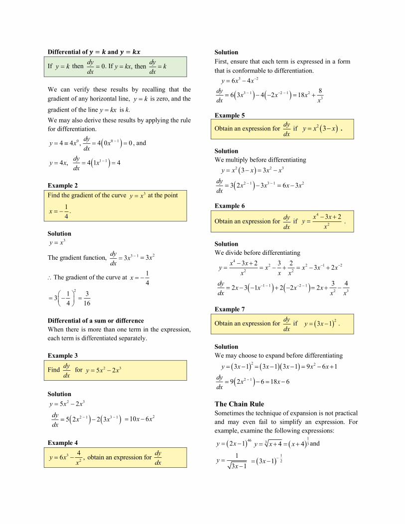
Differential of 𝒚 = 𝒌 and 𝒚 = 𝒌𝒙

If then . If

We can verify these results by recalling that the gradient of any horizontal line, is zero, and the

gradient of the line is k. We may also derive these results by applying the rule for differentiation.

, and

Example 2 Find the gradient of the curve at the point

.

Solution

The gradient function,

The gradient of the curve at

Differential of a sum or difference When there is more than one term in the expression, each term is differentiated separately. Example 3

Find for

Solution

Example 4

Solution First, ensure that each term is expressed in a form that is conformable to differentiation.

Example 5

Obtain an expression for if .

Solution We multiply before differentiating

Example 6

Obtain an expression for if .

Solution We divide before differentiating

Example 7

Obtain an expression for if .

Solution We may choose to expand before differentiating

The Chain Rule Sometimes the technique of expansion is not practical and may even fail to simplify an expression. For example, examine the following expressions:

and

y k= 0dydx

= , then dyy kx kdx

= =

y k=y kx=

( )0 0 14 4 , 4 0 0dyy x xdx

-= º = =

( )1 14 , 4 1 4dyy x xdx

-= = =

3y x=

14

x = -

3y x=

3 13dy xdx

-= 23x=

\14

x = -

21 334 16

æ ö= - =ç ÷è ø

dydx

2 35 2y x x= -

2 35 2y x x= -

( ) ( )2 1 3 15 2 2 3dy x xdx

- -= - 210 6x x= -

32

46 , obtain an expression for dyy xdxx

= -

( ) ( )

3 2

3 1 2 1 23

6 486 3 4 2 18

y x xdy x x xdx x

-

- - -

= -

= - - = +

dydx

( )2 3y x x= -

( )

( )

2 2 3

2 1 3 1 2

3 3

3 2 3 6 3

y x x x xdy x x x xdx

- -

= - = -

= - = -

dydx

4

2

3 2x xyx- +

=

42 2 1 2

2 2

3 2 3 2 3 2x xy x x x xxx x

- -- += = - + = - +

( ) ( )1 1 2 12 3

3 42 3 1 2 2 2dy x x x xdx x x

- - - -= - - + - = + -

dydx

( )23 1y x= -

( ) ( )( )

( )

2 2

2 1

3 1 3 1 3 1 9 6 1

9 2 6 18 6

y x x x x xdy x xdx

-

= - = - - = - +

= - = -

( )462 1y x= - ( )1

3 34 4y x x= + = +

13 1

yx

=-

( )123 1x -= -

If these expressions are expanded the numbers of terms would be large. More so, those with negative and/or fractional indices would have an infinite number of terms. Therefore, we need to find a more efficient way of differentiating this type of expression. The chain rule is used to differentiate such composite functions It is sometimes called ‘function of a function’ and the method is often referred to as the ‘method of substitution’.

If we have a composite function such that

Example 8

Differentiate .

Solution Applying the chain rule, we have:

Example 9

Differentiate .

Solution

The Product Rule The product rule is useful when differentiating a product of two functions and in which a simple multiplication such is not possible. The rule states:

If y is of the form, , then .

It is necessary in cases where the functions u and v cannot be combined with simple multiplication. The Quotient Rule We use the quotient rule when there is a quotient that cannot be simplified using a simple division. The rule states:

If , then .

Example 10 Differentiate . Solution

To determine , we use the chain rule

Let , so

Example 11

Differentiate .

Solution Let and .

( ) and ( )

then by the Chain rule

y f t t g xdy dy dtdx dt dx

= =

= ´

( )102 1y x= -

( )102 1y x= -10

9

Let 2 1, and

2 10

t x y tdt dy tdx dt

= - =

= =

( )99 910 2 20 20 2 1dy dy dt t t xdx dt dx

= ´ = ´ = = -

13 2

yx

=-

( )12

1 3 23 2

y xx

-= = --

12

12 1

Let 3 2 and 1 3 2

t x y tdt dy tdx dt

-

- -

= - =

= = -

( )

1 12

3 3

1 32

3 3

2 2 3 2

dy dy dt tdx dt dx

t x

- -= ´ = - ´

- -= =

-

y uv=dy du dvv udx dx dx

= +

uyv

= 2

du dvv udy dx dxdx v

-=

( )2 1 3 2y x x= + +

Let 2 1 and 3 2

2

u x v xdudx

= + = +

=

dvdx

3 2v x= +

3 2t x= +12v t=

( ) ( )12

1 33 2 32 2 3 2

dv xdx x

-= + =+

( ) 33 2 2 2 12 3 2

6 3 18 112 3 22 3 2 2 3 2

dy du dvv u x xdx dx dx x

x xxx x

= + = + ´ + + ´+

+ += + + =

+ +

4 12 4xyx+

=-

4 1u x= + 2 4v x= -

Applying the quotient law,

,

Example 12 The normal to the curve at the point

crosses the x-axis at A. Find the coordinates of A. Solution

The gradient function of the curve,

The gradient of the tangent at (2, −4) is = 6(2)0 − 10(2) = 4

Hence, the gradient of the normal is (the

product of the gradients of perpendicular lines ).

To find the equation of the normal, we use 𝑦 − 𝑦6𝑥 − 𝑥6

= 𝑚

When .

Therefore, A .

Differentiation as a limit Earlier, we used differentiation to find the gradient of a curve at a point. We did so by obtaining the

gradient function, 121,

which is itself a function that gives us the gradient at any point on the curve. For polynomial functions of the form 𝑦 = 𝑎𝑥% , we simply used the procedure, 12

1,= 𝑛𝑎𝑥%/6.

We will now discover how these procedures were derived through another method.

Using the limit of a chord to find the gradient function Consider the function, . To obtain the differential from first principles of , let us first look at its graph, or more precisely, a section of its graph. For the curve, let P be some arbitrary point

on the curve with coordinates . So, the

coordinates of P in terms of x will be .

Some distance away, say h, to the right of P, we choose another point, Q, on the curve, with the x coordinate of (𝑥 + ℎ). The coordinates of Q will be [(𝑥 + ℎ), (𝑥 + ℎ)0]. We join P to Q as shown in the diagram below.

Now, we now find the gradient of the chord PQ of the curve. Recall the formula for the gradient of a straight line joining the points (𝑥6, 𝑦6) and (𝑥0, 𝑦0) is

𝑚 = 2-/2;,-/,;

, where (𝑥6, 𝑦6) = (𝑥, 𝑥0) and (𝑥0, 𝑦0) = [(𝑥 + ℎ), (𝑥 + ℎ)0]

4dudx

= 2dvdx

=

2

du dvv udy dx dxdx v

-=

( ) ( )( ) ( )2 2

2 4 4 4 1 2 182 4 2 4

x xdydx x x

- - += = -

- -

3 22 5y x x= -

( )2, 4-

3 22 5y x x= -

( ) ( )3 1 2 1 22 3 5 2 6 10dy x x x xdx

- -= - = -

14

-

1= -

( )4 12 4

4 16 24 14

yxy x

y x

- -= -

-+ = - +

= - -

0, 14y x= = -

( )14, 0-

2y x=2y x=

2y x=

( ),x y

( )2,x x

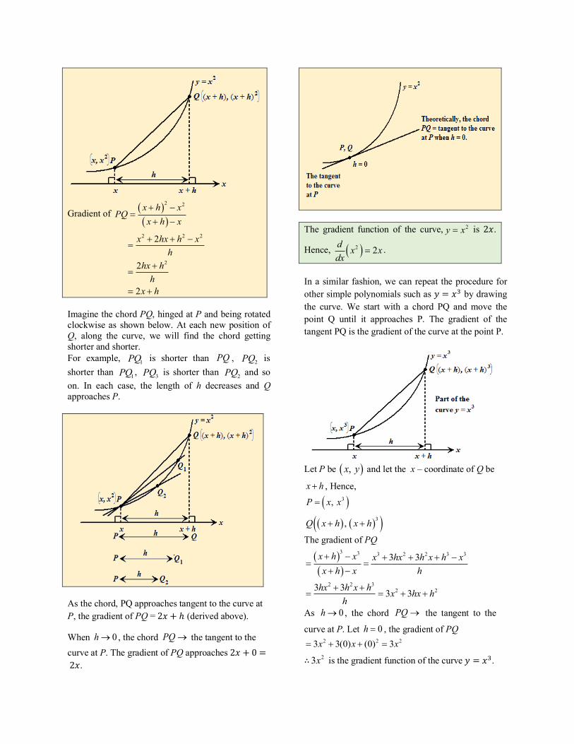
Gradient of

Imagine the chord PQ, hinged at P and being rotated clockwise as shown below. At each new position of Q, along the curve, we will find the chord getting shorter and shorter. For example, is shorter than , is shorter than , is shorter than and so on. In each case, the length of h decreases and Q approaches P.

As the chord, PQ approaches tangent to the curve at P, the gradient of PQ = 2𝑥 + ℎ (derived above).

When , the chord the tangent to the curve at P. The gradient of PQ approaches 2𝑥 + 0 =2𝑥.

The gradient function of the curve, is 2𝑥.

Hence, .

In a similar fashion, we can repeat the procedure for other simple polynomials such as 𝑦 = 𝑥9 by drawing the curve. We start with a chord PQ and move the point Q until it approaches P. The gradient of the tangent PQ is the gradient of the curve at the point P.

Let P be and let the x – coordinate of Q be

, Hence,

The gradient of PQ

As , the chord the tangent to the

curve at P. Let , the gradient of PQ

∴ is the gradient function of the curve 𝑦 = 𝑥9.

( )( )

2 2x h xPQ

x h x+ -

=+ -

2 2 2

2

2

2

2

x hx h xh

hx hh

x h

+ + -=

+=

= +

1PQ PQ 2PQ

1PQ 3PQ 2PQ

0h® PQ®

2y x=

( )2 2d x xdx

=

( ),x yx h+

( )3,P x x=

( ) ( )( )3,Q x h x h+ +

( )( )

3 3 3 2 2 3 3

2 2 32 2

3 3

3 3 3 3

x h x x hx h x h xx h x h

hx h x h x hx hh

+ - + + + -= =

+ -

+ += = + +

0h® PQ®

0h =2 2 23 3(0) (0) 3x x x= + + =23x

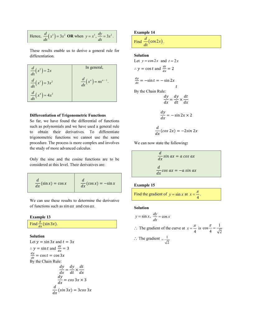
These results enable us to derive a general rule for differentiation.

In general,

.

Differentiation of Trigonometric Functions So far, we have found the differential of functions such as polynomials and we have used a general rule to obtain their derivatives. To differentiate trigonometric functions we cannot use the same procedure. The process is more complex and involves the study of more advanced calculus. Only the sine and the cosine functions are to be considered at this level. Their derivatives are:

𝑑𝑑𝑥 (sin 𝑥) = cos𝑥

𝑑𝑑𝑥 (cos 𝑥) = −sin 𝑥

We can use these results to determine the derivative of functions such as sin𝑎𝑥 and cos𝑎𝑥. Example 13 Find 1

1,(sin3𝑥).

Solution Let 𝑦 = sin 3𝑥 and 𝑡 = 3𝑥

∴ 𝑦 = sin 𝑡 and 1V

1,= 3

121V= cos 𝑡 = cos3𝑥

By the Chain Rule: 𝑑𝑦𝑑𝑥 =

𝑑𝑦𝑑𝑡 ×

𝑑𝑡𝑑𝑥

𝑑𝑦𝑑𝑥 = 𝑐𝑜𝑠 3𝑥 × 3

𝑑𝑑𝑥 (𝑠𝑖𝑛 3𝑥) = 3𝑐𝑜𝑠3𝑥

Example 14

Find .

Solution Let and

∴ 𝑦 = cos 𝑡 and 1V1,= 2

121V= −sin 𝑡 = −sin 2𝑥

𝑡 By the Chain Rule:

𝑑𝑦𝑑𝑥 =

𝑑𝑦𝑑𝑡 ×

𝑑𝑡𝑑𝑥

𝑑𝑦𝑑𝑥 = −sin2𝑥 × 2

𝑑𝑑𝑥(𝑐𝑜𝑠2𝑥) = −2𝑠𝑖𝑛2𝑥

We can now state the following:

𝑑𝑑𝑥 𝑠𝑖𝑛𝑎𝑥 = 𝑎𝑐𝑜𝑠𝑎𝑥

𝑑𝑑𝑥 𝑐𝑜𝑠𝑎𝑥 = −𝑎𝑠𝑖𝑛𝑎𝑥

Example 15

Find the gradient of at .

Solution

,

The gradient of the curve at is

The gradient

( )2 2d x xdx

=

( )3 23d x xdx

=

( )4 34d x xdx

=

( ) 1n nd x nxdx

-=

( )cos2d xdx

cos2y x= 2t x=

siny x=4

x p=

siny x= cosdy xdx

=

\4

x p=

1cos4 2p=

\ 12

=

Hence, OR when . ( )3 23d x xdx

= 3 2, 3dyy x xdx

= =