Agent-Based Models:A New Challenge for Statisti s

David Banks

Duke Uniffirsity

1

1. History of Agent-Based Models (ABMs)

ABMs arise in omputer experiments in whi h it is possible to de�ne intera tions�lo ally� for ea h agent, and then simulate emergent behavior that arises from theensemble of lo al de isions.Examples in lude:

• Weather fore asting, in whi h ea h agent is a ubi kilometer of atmosphere, andthe lo al intera tions are ex hange of pressure, temperature, and moisture.

• Au tions, as in Yahoo! or Google, to determine whi h ads are shown to users.

• Tra� �ow models, as in TRANSIMS, where agents (drivers) spa e themselvesa ording to the a tions of other drivers, and make route hoi es based on ongestion avoidan e.• Geneti algorithms.Often the lo alization is geographi , but this is not essential. The au tion examplehas no spatial omponent.

2

ABMs began in the 1940s, with ideas by von Neumann and Ulam relating to ellularautomata (obje ts whi h, under a �xed set of rules, produ e other obje ts, usually onpaper grids�the most famous example is J. H. W. H. Conway's Game of Life).This led to mathemati al theories of intera tive parti le systems (Frank Spitzer,David Gri�eath), whi h used methods from statisti al me hani s to study problemsrelated to phase hanges and system dynami s.As the agents developed more omplex rules for intera tion, and as the appli ationsbe ame more tuned to simulation studies of observable phenomena, the �eld morphedaway from mathemati s into e onomi s, so ial s ien e, and physi s.These models are popular be ause they enjoy a ertain fa e-validity, and be ause theyare often easy to program.

3

ABMs are omputer-intensive, and so did not be ome widely used until the 1990s. Amajor impetus was Growing Arti� ial So ieties, by Joshua Epstein and Robert Axtell(1996, MIT Press). This book showed how simple and interpretable rules for agents ould simulate behavior that was interesting in demography, anthropology, so iology,and e onomi s.Their approa h was to posit a sugars ape, a plane on whi h, at ea h grid point,�sugar� grew at a onstant rate. Agents had lo ations on the sugars ape, and onsumed the sugar at their lo ation until it was exhausted, and then moved to a newlo ation (in the dire tion of maximum sugar, without diagonal moves, with minimumtravel and a preferen e to be near previous lo ations).This simple system of rules led to ir ular migration patterns. These patterns aresupposed to be similar to those observed in hunter-gatherer populations.

4

More rules reated additional omplexity. Epstein and Axtell added sex, and whenthere was su� ient sugar, the agents would reprodu e. This led to age pyramids, arrying apa ity, tribal growth with o-movement and �ssion, and other demographi features.They added �spi e�, a se ond resour e similar to sugar, and simple rules led to bartere onomies.They added �tags�, whi h are shared in a tribe under majority rule. These tags mimi ultural memes, and are transmitted and onserved. When tags are asso iated withsurvival and reprodu tive su ess, the tribes show Spen erian ultural evolution.Similar rules led to ombat, division of labor, disease transmission, and otherevo ative results.

5

Spa ing of agents, su h as would o ur with hunter-gatherers.

6

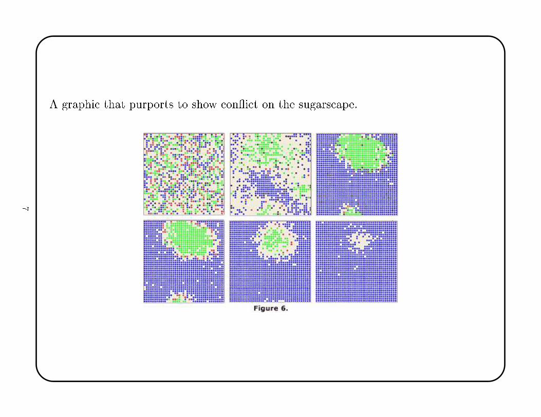
A graphi that purports to show on�i t on the sugars ape.

7

Currently, ABMs typi ally entail:1. Many agents, often with di�erentiated roles and thus di�ent rule sets.2. Rules, whi h may be omplex. Sometimes the rules are heuristi , sometimes onehas randomized rules.3. Learning and adaptation. Agents learn about their environment (in luding otheragents). (Axelrod's Prisoner's Dilemma is an example.)4. An intera tion topology. This de�nes whi h agents a�e t ea h other�usually thisis a model of propinquity, but for au tions it is a star-graph.5. A non-agent environment. This may in lude initial onditions, and/or ba kgroundpro esses.Sin e the 1990s, most simulations use smart agents with multiple roles. Currentwork is exploring how well agents that implement models for human ognition (e.g.,bounded rationality) an reprodu e empiri al e onomi behavior.

8

2. Kau�man's Model

Stanley Kau�man wanted to know how DNA ould give rise to the number of di�erenttissue types that are observed in organisms. He performed an ABM experimentdes ribed in �Metaboli Stability and Epigenesis in Randomly Constru ted Geneti Nets�.In Kau�man's model, ea h agent is a gene. Ea h gene is either o� or on, 0 or 1,depending upon the inputs it re eives from other genes. Genes re eive inputs fromother genes, al ulate a Boolean fun tion, and send the result to other genes.If a gene re eives k inputs, then there are 2k possible ve tors of inputs. And for ea hgiven ve tor of inputs, there are two possible outputs, 0 or 1. So the number ofpossible fun tions that map {0, 1}k → {0, 1} is 22k .

9

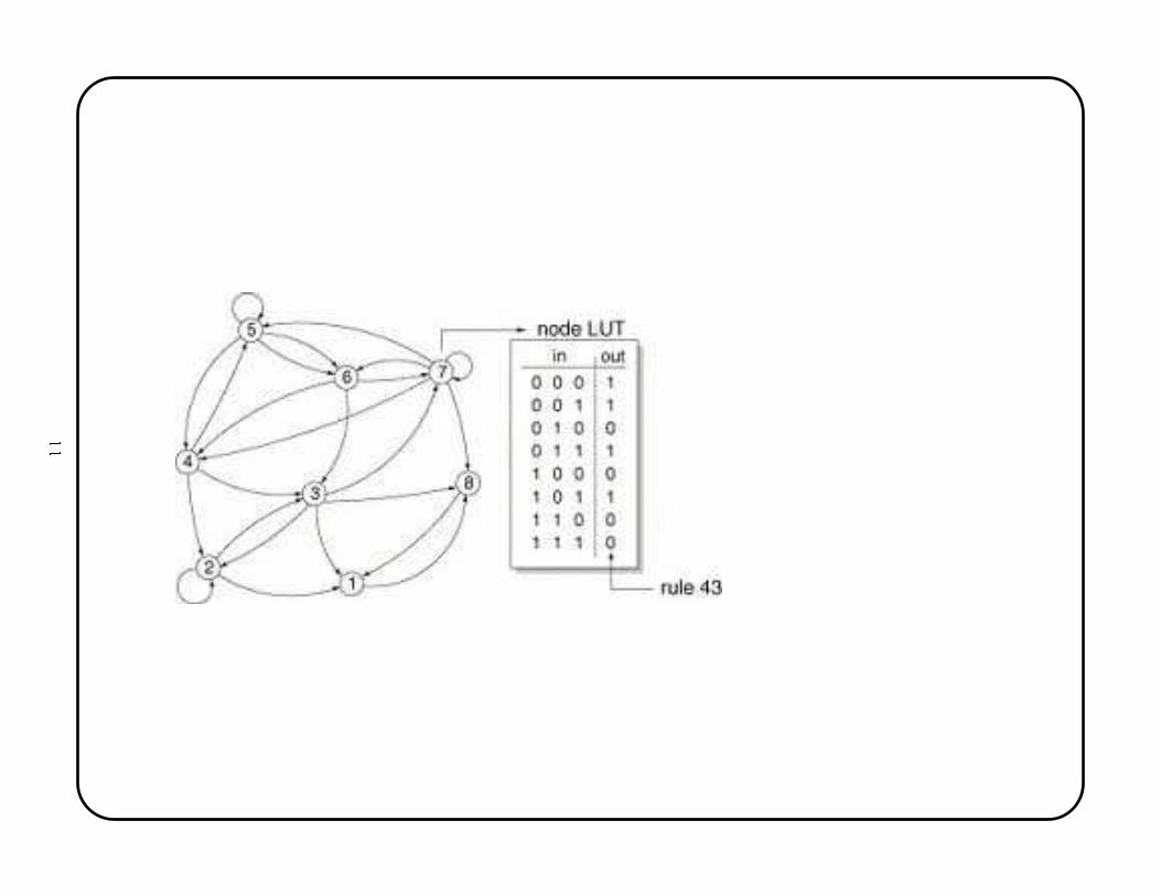
A network of eight nodes, in whi h genes have di�erent numbers of inputs andtransmit to di�erent numbers of genes. Gene 7 re eives input from genes 3, 6 and 7(itself), and sends to gense 5, 6, 7 and 8.10

11

Given a network of n genes that are randomly onne ted and for whi h ea h gene is arandomly hosen Boolean fun tion, it turns out that the system must always develop y les. The on-o� patterns will typi ally move through a set of transient states, andultimately settle upon a y le, whi h is alled an attra tor.The number of attra tors is typi ally about equal to √n. Whi h attra tor one endsup in depends upon the initial onditions.Biologi ally, one an imagine that ea h attra tor orresponds to a tissue type. Aparti ular sequen e of gene regulation, turning spe i� genes o� and on in a regular y le, determines whether the ell is a nerve ell or a skin ell.This isn't true, of ourse, but it is a suggestive model for how the same DNA anprodu e di�erent out omes.

12

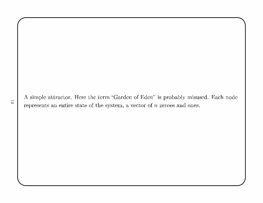
A simple attra tor. Here the term �Garden of Eden� is probably misused. Ea h noderepresents an entire state of the system, a ve tor of n zeroes and ones.13

14

Interestingly, random networks tend to be robust. If one randomly perturbs thenetwork by �ipping a 0 to a 1, or a 1 to a 0, then nearly always you �nd yourself upona transient that leads ba k to the original attra tor.Of ourse, with small probability, sometimes a �ipped bit or two will put one on atransient path that leads to a di�erent attra tor. This is similar to what happens inbiology, where sometimes one �nds aberrant tissue types in the wrong organ.Of ourse, in biology, natural sele tion operates on the pro ess so that the genes arenot randomly onne ted and do not have random Boolean fun tions. Instead, therewould be sele tion for on�gurations that are stable and have many domains ofattra tion.15

The verti al axis shows the number of attra tors and number of ell types, and thetop horizontal axis shows the number of agents while the bottom horizontal axisshows the amount of DNA.16

17

3. Veri� ation and Validation

The validation problem is to determine whether the program is su� ientlyfaithful to reality. Simulation models make many di�erent kinds of assumptions andapproximations, and often the result is ompletely unsound, even if the ode iserror-free. To make things more di� ult, often one has very little data from the realworld against whi h to ompare the model.In this ontext, the veri� ation problem is to determine whether the ode in themodel is error-free. It is impossible to he k every line of ode, and one an essentiallyguarantee that in programs with millions of lines, written by hundreds of people overde ades, some of the ode will be wrong.Both of these problems are largely intra table. But the need for modeling is great,and often the solution is fairly robust within regions that people are about. Andstatisti s has some partial assistan e it an o�er.

18

3.1 Validation Strategies

There seem to be �ve main approa hes:

• Physi s-based modeling

• Intelligent design

• Fa e-validity

• Comparison to another model• Comparison to the worldRegrettably, none of these is fully satisfa tory.Re ent statisti al work based on a model for dis repan y developed by Kennedy andO'Hagan (Bayesian Calibration of Computer Models, a read paper in Journal of theRoyal Statisti al So iety, Ser. B, 63, 425-464) may o�er a useful path forward insome situations.

19

3.1.1 Physi s-Based Modeling

This method is ommonly used in the hard s ien es. People build a simulation thatin orporates all of the physi al laws and intera tions that they an think of, and thenfeel on�dent that their model is faithful to reality.This an work on smaller problems where all me hanisms are fully understood.Examples where it is arguably su essful in lude planetary motions, �ight simulators,and virtual mo k-ups of semi ondu tor manufa turing pro essesBut it tends to break down as the sto hasti ity of the problem in reases. And themi ro-level simulations often take a very long time to run.

20

3.1.2 Intelligent Design

This is the most ommon. Experts think through the simulation arefully, buildingin or approximating all the e�e ts they think are substantial. Then they hope thatthey've been smart enough and wait to see if their results work well enough.This is probably the ase with most simulations that are not mission- riti al.Intelligent design an handle more ompli ated situations that the physi s-basedmodels, but there is no true validation.Mu h of the ode written by government ontra tors is designed this way, largelybe ause higher levels of validation testing are expensive and federal agen ies arerelu tant to pay for it.Sin e the thought-pro ess is similar to software design, the results are probably aboutas buggy as ode.

21

3.1.3 Fa e-Validity

This is the �rst ase with a true validation proto ol. The designer tests the simulationby using sele ted inputs to explore the output behavior.Often the sele ted inputs are hosen a ording to a statisti al design, su h as a Latinhyper ube. This is a bit more e� ient. Alternatively, one an try to sele t values forthe inputs that orrespond to expe ted behaviors.This is insu� ient when the parameter spa e is large and there are many intera tions.But, to varying degrees, it is used for systems su h as EPISIMS and the battle�eldsimulations produ ed at DMSO.Fa e-validity assessment requires signi� ant in-house expertise with both the softwareand the appli ation.

22

3.1.4 Comparison to Another Model

This is not done often enough, but it has the potential to be a powerful tool forvalidation. The advantages are that one an better explore the full range of modelbehavior.One issue is that it is hard to de ide when one simulation is nearly equivalent toanother, or perhaps is a subset of the other. And it an be espe ially important if oneof the simulations runs very mu h faster than the other; for example, one an use theslow one that is possibly more a urate as an an hor for alibrating and fast one.Su h omparative validation an arise when examining the Reed-Frost di�erentialequations for disease spread against, say, an agent based model.

23

3.1.5 Comparison to the World

For many situations, su h as weather fore asting and the HAZUS �ood damagemodel, the users an ompare predi tions with what was later observed.Although this is probably the strongest form of validation, it is still inadequate. Onedoes not have on�den e in the �delity of the simulation in regimes that have not beenpreviously observed, and this is often the ontext when there is the greatest interest.Also, when there is randomness, it is di� ult to quantify the strength of supportobtained by orre t or in orre t predi tions.

24

3.2 Veri� ation

Finding the bugs in ode is an entirely di�erent but very di� ult problem.One approa h is to he k every bran hpoint in the program to ensure that the logi issound. Software quality engineers a tually do this.Perhaps less ostly is to hire two people to independently write ode with pres ribedmodularity, then set a lot of little internal �ags, and then run inputs to see where the�ags disagree. When that happens, one of the programmers has made an error. (Of ourse, this more than doubles the upfront ost of ode produ tion.)Resear h at the Software Engineering Institute suggests some subparts ofprogramming tasks are espe ially error-prone, and some programmers are apt to ertain kinds of errors (Watts Humphrey, many SEI reports).Mathemati ians have developed a theory of provably orre t ode, but is not pra ti al.

25

Other people have used lever statisti al designs to help ensure diverse testing withoutthe ost of exhaustive testing (e.g., Dalal and Mallows (Te hnometri s, 40, 234-243).Another paper by Dalal and Mallows (JASA, 83, 872-880) is even better. This usesdynami programming, the ost of the bugs that have been found, the ost of testing(in luding opportunity osts from delayed release) and the length of time sin e �ndingthe last bug to �nd the optimal time to stop testing.The intuition is lear: if it has been a long time sin e you last found an expensivebug, then de lare the ode ready for market.None of these methods is fully satisfa tory for life-or-death ode. This hearkens ba kto elementary statisti s: you annot prove the null hypothesis that the ode is good,you an only disprove it.

26

4. Parameterization

To improve validation, we need to understand the parameter spa e. All simulationshave parameters, but these are often hosen for ease of development rather than fortesting and omparison.

• For mathemati al models, the parameters are the oe� ients and the seeds.

• For agent-based models, there are parameters for ea h agent, representing therules that agent follows.• For red-teaming, the parameters are the initial information and the temperamentsof the parti ipants.Similarly, the parameter spa e of the real-world phenomenon needs to be understood.Often the behavior of interest is globally high-dimensional but lo ally low-dimensional.

27

4.1 SIR Models

Consider an old-fashioned di�erential equations model for disease spread. TheKerma k-M Kendri k model assumes:

dI

dt= λIS − γI

dS

dt= −λIS

dR

dt= γI

Here I(t) is the number of infe ted people, S(t) is the number of sus eptible people,and R(t) is the number of people who have re overed and are immune. The λ is theinfe tion rate and γ is the re overy rate.This is a ompartmental model with three ompartments�infe ted, sus eptible, andre overed. The model does not �t data espei ally well, but it represents a standardapproa h for des ribing a simple onta t pro ess.

28

It is lear that the intrinsi dimension of the Kerma k-M Kendri model is 2.Knowing this enables analysts to explore the simulation spa e by varying these twoparameters, λ and γ, and studying how the response (say, duration of the epidemi )depends on these values.In ontrast, many ABM simulations have been developed for this appli ation. Agentswalk around a spa e, infe ting ea h other with a ertain probability, and analystsexamine the duration.The ABM simulation is not ompletely equivalent to the di�erential equationmodel�the disease an burn out before the entire population has ontra ted it.Nonetheless, qualitatively, the two models are extremely similar.ABM users do not realize that their model is essentially two-dimensional.

29

4.2 Estimating Intrinsi Dimensionality

The dimensionality of a model is a key property that drives inferen e and governs omplexity. In general, an ABM analysis does not know the intrinsi dimension of thedata. It is related to the rule set, but that relationship is usually un lear.One would like a way to estimate the intrinsi dimension of an ABM. For the diseasetransmission example, the parameter spa e is IR+ × IR+, but in more omplexappli ations the spa e will be more omplex (often a Cartesian produ t of intervalsand nominal values).When the intrinsi parameter spa e is a onvex subset of a Eu lidean spa e, thenone an probably estimate the dimensionality by prin ipal omponents regression(PCR). For example, one starts the ABM with many di�erent values for movementand disease transmission, re ords the duration of the epidemi , and then does PCRto �nd the number of omponents required to explain a substantial fra tion of thevariability in the response.

30

However, the intrinsi parameter spa e is probably not usually a onvex subsetof a Eu lidean spa e. But it may still be possible to get an estimate of the lo aldimensionality of the ABM.Run the AMB many times. Let yi be the output of interest for run i, say the durationof the epidemi . And let xi ∈ IRp be all the tunable parameters in the ABM (e.g.,infe tiousness, mixing, family sizes, et .). Then iterate the following steps M times.1. Sele t a random point X∗

m in the onvex hull of x1, . . . ,xn, for m = 1, . . . ,M2. Find a ball entered at X∗ that ontains exa tly k points (say k = 4p).3. Perform a prin ipal omponents regression on the k points within the ball.4. Let cm be the number of prin ipal omponents needed to explain a �xedper entage (say 80%) of the varian e in the yi values.The average of c1, . . . , cM may be a useful estimate of the average lo al dimension ofthe ABM model.

31

This heuristi approa h assumes a lo ally linear fun tional relationship for pointswithin the ball. The Taylor series motivates this, but the method will break down forsome pathologi al fun tions or if the data are too sparse.To test the approa h, Banks and Olszewski (2003; Statisti al Data Mining andKnowledge Dis overy, 529-548, Chapman & Hall) performed a simulation experimentin whi h random samples were generated from q- ube submanifolds in IRp, and theapproa h des ribed above was used to estimate q.A q- ube in IRp is the q-dimensional boundary of a p-dimensional ube. Thus:

• a 1- ube in IR2 is the perimeter of a square,• a 2- ube in IR3 are the fa es of a ube,• a 3- ube in IR3 is the entire ube.

32

The following �gure shows a 1- ube in IR3, tilted 10 degrees from the natural axes inea h oordinate.

33

The following �gure shows a 1- ube in IR10, tilted 10 degrees from the natural axes inea h oordinate.0.0 0.2 0.4 0.6 0.8 1.0

0.1

0.2

0.3

0.4

0.5

0.6

0.7

Dia onis and Freedman (1984; Annals of Statisti s, 12, 793-815) show that inhigh-dimensions, nearly all proje tions look normal.

34

The simulation study generated 10 ∗ 2q points at random on ea h of the 2p−q

(

p

q

)

sides of a q- ube in IRp. Then iid N(0, .25I) noise was added to ea h observation andthe prin ipal omponents approa h was used to estimate q for all values of q between1 and p for p = 1, . . . , 7.The following table shows that the method was reasonably su essful in estimatingthe lo al dimension. The estimates are biased, sin e the prin ipal omponentsanalysis identi�ed the number of linear ombinations needed to explain only 80% ofthe varian e. One should probably do some kind of bias orre tion to a ount for theunderestimate.Note: This example does prin ipal omponents analysis rather than prin ipal omponents regression, but the on ept is straightforward.Note: It seems unlikely that the map from the ABM rule set to the intrinsi parameter spa e to the output is everywhere high-dimensional. If it is, then there isprobably not mu h insight to be gained.

35

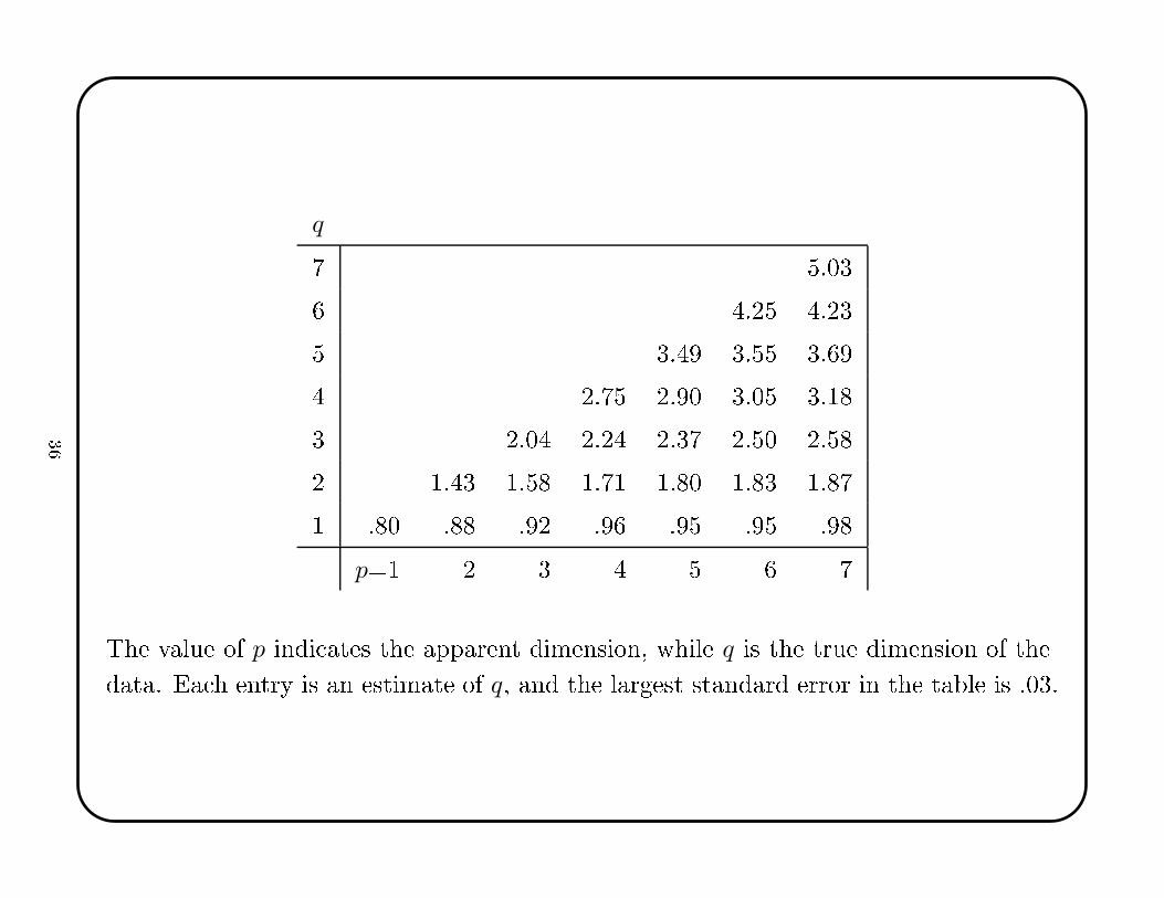
q7 5.036 4.25 4.235 3.49 3.55 3.694 2.75 2.90 3.05 3.183 2.04 2.24 2.37 2.50 2.582 1.43 1.58 1.71 1.80 1.83 1.871 .80 .88 .92 .96 .95 .95 .98

p=1 2 3 4 5 6 7The value of p indi ates the apparent dimension, while q is the true dimension of thedata. Ea h entry is an estimate of q, and the largest standard error in the table is .03.

36

4.3 The Bad Seed

A spe ial kind of parameter is the seed, whi h is arises in all omputer simulationsfor whi h randomness o urs.The seed drives the random number generator, and the generator is hosen to beextremely sensitive to the seed. One wants small hanges in the seed to ause large hanges in the sequen e of generated random variables. (In haos theory, this is alled�sensitive dependen e to initial onditions� or the Butter�y E�e t.)This extreme sensitivity makes some portions of the validation more di� ult. Twosu essive runs might (properly) give answers that are wildly di�erent. But forvalidation, it is better to have smooth dependen e on the seed, so that one an:

• more qui kly explore the set of out omes• e� iently estimate the han e of a given out ome.

37

4.4 Parameterization Summary

Validation is easiest when the parameter set for the simulation is• a onvex subset of a Eu lidean spa e,

• smoothly related to the outputs

• low-dimensional.The �rst two onditions enable one to explore the response as a fun tion of the inputspa e. If one gets unbelievable responses, then there is a validation problem.The last ondition refers to the Curse of Dimensionality. If the truerelationship between the parameter spa e and the out ome of interest is everywherehigh-dimensional, then one an never hope to observe enough data to learly validateperforman e. But often the relationship is lo ally low-dimensional.As a related point, one an determine whether uniform measure on the onvex setassigns orre t probabilities to the out omes. If not, tuning is needed.

38

5. Comparing Models

If two models have �true� parameter spa es with di�erent dimensions, then they arenot equivalent. But one model might be a subset of the other.How an one determine the �true�dimension? One approa h is to use prin ipal omponents regression. Sample the inputs at random, and use PCR to �t the outputs.The number of omponents needed to explain 95% of the variation is a measure of thedimension.Given previous omments about lo ally low-dimensional relationships, probably oneneeds to do this separately within di�erent small regions of the input spa e.But this measure overlooks nonlinearity and intera tions, both of whi h are key toimportant problems. I suspe t Random Forests may o�er an alternative.

39

Suppose one has two simulators, both of whi h produ e the same set of out omes. Forthe same out ome, in prin iple one ould look at the preimages in the parameterspa e for both. If sets of preimages have di�erent topologies, then the simulators haveto be di�erent.When the simulators are sto hasti , it will be even more di� ult to �nd thepreimages (one should regard the seed as a parameter). This may lead to probabilisti statements about the degree of similarity between two simulators.In pra ti e, many simulators are written in modular units. Sometimes one might beable to apply validation strategies to ea h module separately, and then validate ormessage-passing network between the modules.

40

6. Model Calibration

Work in limate fore asting at NCAR and explosion simulation at LANL has led to anew approa h to alibrating omputer models. This is losely related to validation,and the new theory is pertinent to ABMs.The alibration approa h is useful when one has a omplex ABM that takes a longtime to run, but there is some real-world experimental data whi h an be used totune the model.The goals are to:

• use the experimental data to improve the alibration parameters (i.e., the rulesets);

• make predi tions (with un ertainty) at new input values;

• estimate systemati dis repan ies between the ABM and the world.

41

Suppose that at various settings of the rule-based input values x1, . . . ,xn one anobserve real world responses y1, . . . , yn. Let

yi(xi) = ψ(xi) + ǫ(xi)where ψ(xi) denotes the real or expe ted response of the world and ǫ(xi) denotesmeasurement error or random disturban e.The observed data are then modeled statisti ally using the simulator η(xi,θ) at thebest alibration value θ as:y(xi) = η(xi,θ) + δ(xi) + ǫ(xi)where the random term δ(xi) a ounts for the dis repan y in the simulator and θ isthe best, but unknown, setting of the alibration inputs t.

42

Additionally, one also has supplementary data in the form of simulation resultsη(x∗

j , t∗

j ), for j = 1, . . . ,m. Typi ally the ABM ode takes a long time to run, so m issmall.The Kennedy-O'Hagan approa h s ales all inputs to the unit hyper ube. Then theBayesian version uses a Gaussian pro ess to model the unknown fun tion η(·, ·).In most of the work so far, the Gaussian pro ess has a onstant mean fun tion and aprodu t ovarian e with power exponential form. (See Higdon et al., JASA 2008.)Cov[(x, t), (x′, t′)] = λ−1η R((x, t), (x′; ρη)where λη ontrols the marginal pre ision of η(·, ·) and ρη ontrols the strength ofdependen y in ea h omponent of x and t.It is often useful to add a little white noise to the ovarian e model to a ount forsmall numeri al �u tuations (from, say, adaptive meshing or onvergen e toleran es).

43

The formulation of the prior is ompleted by spe ifying independent priors for theparameters ontrolling η(·, ·): the µ, λη, and ρη.A similar Gaussian pro ess model is used for the dis repan y term δ(x). This hasmean zero and ovarian e fun tionCov(x,x′) = λδR((x,x′); ρδ).

This is a bit athleti , and one might wonder whether the approa h is a tually buyingany redu tion in the overall ost of simulation or un ertainty about the omputermodel. But this stru ture allows one to do Markov hain Monte Carlo sampling toestimate the posterior distribution.

44

In parti ular, one gets posterior distributions for:

• the η(x, t), whi h is the hard-to-know impli it fun tion al ulated by the ABM;• the optimal alibration parameter θ;

• the alibrated simulator η(x,θ);

• the physi al system ψ(x); and

• the dis repan y fun tion δ(x).The latter, of ourse, is most interesting from the standpoint of model validation.When and where this is large points up missing stru ture or bad approximations.In parti ular, iterated appli ation of this method should permit su essive estimationof the dis repan y fun tion. One winds up with an approximation to the ABM interms of simple fun tions, and the a ura y of the approximation an be improved tothe degree required.

45

7. Un ertainty Assessment

One wants to be able to make probability statements about the output of an ABM.For example, if the ABM predi ts that 5,000 people will die of the �u in 2010, it ishelpful to have some error bars.Fortunately, this aspe t of ABMs may be fairly straightforward. As in traditionalstatisti al simulations, one puts a subje tive distribution over ea h of the inputparameters (in the ABM ase, these are the tunable values in the rules). Thenone makes multiple runs, and uses the standard deviation of the results to makeun ertainty statements.However, this addresses only part of the un ertainty in an ABM�the portion thatrelates to the tunable parameters. It does not address model un ertainty.

46

Model un ertainty is a standard problem in statisti al inferen e. For ABMs,model un ertainty relates to whi h rules agents should follow, rather than tunableparameters embedded in the rule.To be lear, in the ontext of disease, one might have a rule that agents onta t aPoisson number of people per day, with the mean of the Poisson being a tunableparameter.But one might onsider adding an additional rule�say that people intera tpreferentially within a so ial network, rather than meeting people at random. Modelun ertainty pertains to whether or not this rule should be in luded in the ABM.The usual �x is to use an ensemble, in whi h there are many di�erent models, andtheir predi tions are weighted a ording to their predi tive a ura y and mutual orrelations. Compared to standard appli ations, ABMs may have an advantage inthat in reasing omplexity is �nested�, and overly omplex rules will not a�e t thepredi tion.47

8. Con lusions• ABMs are an important new tool in simulation; starting in the 1990s, they havebe ome a standard te hnique.

• Statisti al theory for ABMs is almost non-existent. We need to pay attention tothis, and we have tools that may improve ABM methodology.• A key step in a formal ABM theory is a better understanding of theparameterization. Probably one wants a map from IRp to the input spa e, whi hthe simulator then maps to the output spa e. But the �rst map will be weird.

• A se ond key step is the development of alibration methods for ABMs�rightnow, users rely upon fa e validity, and an miss important stru ture.

• A third key step is un ertainty expression. All simulations en ounter this, butABM users have been slow to address it.• Relevant statisti al theory has been or is being developed.

48