M, 55"]

”-5355...5‘0"”.‘5‘""03“."(3" -n ‘v

"' #355 . ‘5

3;"- '5‘"

.El

' 551:, ‘HI'

' 5' 5"”:

1W

-\'n .

15551975.-

‘ 31:33

”3'45. qu ' '\‘'36“

‘3:-33“fix35593355 (\‘yAL‘J35???'53:};

""14"-'1'.-315:3-"3"‘F-I3'";

" we:Egg,:9«533

V125" "‘ ‘“35' ‘ ...

2‘,-ML"$53":55“?:31»39:5“ '5“..%n}. 'l'_ u'

I:

f’

.'"i

‘

55'”

‘‘gfxttg

454

I

5,-5’

L‘.

So

..5

”3-3

-

'_:_

Z

'3

«‘3

t‘ ‘ “I;

(‘55'

:3“‘25 ”if ,

w:“73;?A.§&\§? {-éfitigf‘cufi}

3J1;v‘¢\4!“ '6'. ‘ v . ._ ‘at.Y" ‘Q ‘

.3 .

;_.vf

5.

11‘.'

4'l.

-y‘

5:9:

-5

:\‘_J.'.

~.

We“

'

J“5,3.

-'

.o

‘I

‘-

—

.-J

.‘

.—~.—4..“*Wfl—sr-

5:5. | 555.4

_;l I,“ ‘ 1‘ I.":LVJIE

if. (Lihkl' :H'V

WWHIWWII/Will”MM/WT“0064 5451

u ’5 - ‘ ~. £FW 0'4 smart-ve- '1

This is to certify that the

dissertation entitled

Short-term Growth of an Undisturbed

Tropical Moist Forest in the Brazilian

Amazon

presented by

Niro Higuchi

has been accepted towards fulfillment

ofthe requirements for

PhD degreein Forestry

55/

Major professor

Date {/1 31/6?

MSU i: an Alfmmm‘n Action/Equal Opportunity Institution042771

MSU

RETURNING MATERIALS:

Place in book drop to

remove this checkout from

LIBRARIES

All-(gulls.your record. FINES will

be charged if book is

returned after the date

stamped below.

”UN 1 1 19.0.0.

‘ 17:1"'~¢’

, 1'-

}J

r-

I‘l

I. v 1

I f '

l

f‘rfi E-‘k’.

“Anya “

55.

mt! 21 “3“}?

E . 2%55

SHORT-TERM GROWTH OF AN UNDISTURBED TROPICAL MOIST FOREST

IN THE BRAZILIAN AMAZON

BY

Niro Higuchi

A DISSERTATION

Submitted to

Michigan State University

in partial fulfillment of the requirements

for the degree of

DOCTOR OF PHILOSOPHY

Department of Forestry

1987

IHEHRACT

SHORT-TERM GROWTH or AN uuoxsruaaeo TROPICAL uorsr FOREST

IN THE BRAZILIAN amazon.

by

NIRO HIGUCHI

The main objective of this study is to provide basic

information for sustained yield management of the tropical

moist forest in the Brazilian Amazon. This was done by

quantification of diameter distributions, projections of

Idiameter distributions and of tree mortality, and by

development of short-term growth and yield models.

The data for this study were collected from an

undisturbed stand located some 90 kilometers north of

Manaus, the capital of Amazonas State - Brazil. Three

permanent plots were established in 1980 and remeasured in

1985. They are the control plots of a forest management

experiment randomly replicated within an area of about 2,000

hectares of pristine Amazonian forest. In each 4-hectare

plot (200 by 200 meters), all trees with dbh 25 cm or

greater were tagged and their dbhfls were recorded in 1980.

In 1985. all tagged trees were remeasured with special

attention to ingrowth and mortalityu The number of trees,

dbh and basal area of the study area averaged 158 trees/ha.

ii

38 cm, and 20 mZ/ha, respectively - in 1980.

Among three different hypothesized diameter

distribution functions, the Weibull using the percentile

approach best fit the observed data. 3

Since age and successive records from long-term

permanent plots were not available, the first-order Markov

chain approach was used to project diameter distribution and

tree mortality and proved to be a realistic alternative.

The exponential Lotka growth model was adapted to

predict future volume as an alternative for the traditional

growth and yield models, and it behaved satisfactorily. The

volume for 1990 was also predicted by models based upon the

volume estimated in 1985 in relation to the dbh measured in

1980. There was a strong correlation between actual volume

and past dbh, but not between past diameter and diameter

growth.

iii

To

Inezita and Chico, and Maria

my children, my wife - my friends

iv

ACKNOWLEDGEMENTS

I wish to express my gratitudetto Dr. Carl W. Ramm.

Chairman of my dissertation committee, for his insight,

support, and guidance in the preparation of this work. I

also wish to extend my gratitude to Dr. Lee M. James, Dr.

Kurt S. Pregitzer and Dr. Peter G. Murphy for serving on my

guidance committee and assisting throughout my doctoral

program.

I would like to extend my acknowledgements to Dr. Phu

Nguyen, Mr. T. W. W. Wood, Dr. Jurandyr C. Alencar, Dr. Kurt

S. Pregitzer, Dr. Lee M. James, and Dr. Carl W. Ramm. They

provided helpful suggestions on an earlier version of

specific chapters of this manuscript .

I would like to pay special tribute to my wife, my kids

and my "pessoal" from Chavantes and Chapeco for their

encouragement, patience and supportive "rezas".

I am indebted to many people whose friendship was

important during the course of this voluntary exile. Thank-

you to Antonio & Lucia, Josmar & Fernanda, Carlos, Steve

Westin, Robert De Geus, Bill Cole, Don Zak and George Host.

I would like to express my sincere gratitude to Luis

Maurc>& Fatima Magalhaes for being my proxy in Brazil and

for their patient support during this time.

Special thanks are due to the "peaozada" of DST

(Departamento de Silvicultura Tropical)-Aluizhm5Cabore,

Jesus, Barrao, Caroco, Paulista, Armando and other anonymous

helpers - who have been my great masters in the forest and

particularly for their help during field data collection. I

also wish to thank the group of DST's "pica-pan" - Fernando,

Antenor, Jurandyr, Magalhaes, Benedito, Noeli and Joaquim -

who played an important role during the preparation of this

research project. I am also indebted to many people from

other departments of INPA for their support. Thank-you to

"turma" of administration and to Nakamura.

I gratefully acknowledge the support of many staff

members of the Department of Forestry of Michigan State

University.

Finally, my sincere appreciation to my country - Brasil

- through CNPq (Conselho Nacional de Desenvolvimento

Cientifico e Tecnologi'co) for financial and administrative

support, and INPA (Instituto Nacional de Pesquisas da

Amazonia) for inspiration.

THANK YOU GOD !

vi

TITLE . .

ABSTRACT

DEDICATION

ACKNOWLEDG

TABLE OF C

TABLE

EMENTS O O O C

ONTENTS O O O 0

LIST OF TABLES . . . . .

LIST OF FI

CHAPTERS

1. INTRODU

Scepe

GURES O O O O

CTION O O O O O

of the Problem

OF CONTENTS

Statement of the Problem . . . .

2. LITERATURE REVIEW ON THE MANAGEMENT

REGENERATION IN THE TROPICAL MOIST FORESTS

2.1.

2.2.

2.3.

2.4.

2.5.

2.5.

2.7.

Overview . . .

Introduction . .

Tropical America

Tropical Africa

Tropical Asia .

Tropical South Pacific . . .

Conclusion . . .

vii

OF NATURAL

page

ii

iv

vii

xiii

03010101

12

13

16

16

3. THE BRAZILIAN AMAZON . . . . . . . . .

3.1. Introduction . . . . . . . . . . .

3.2. Climate . . . . . . . . . . . . .

3.3. Soils . . . . . . . . . . . . . .

3.4. Vegetation . . . . . . . . . . . .

Tropical moist forest on "terra firme"

Inundated forests . . . . . . . .

"Campina" and "Campinarana" . . .

Tropical semi-evergreen forest . .

"Cerrado" (Savannas) . . . . . . .

4. DESCRIPTION OF THE STUDY AREA . . . . . .

5. MODELLING THE DIAMETER DISTRIBUTION OF AN

UNDISTURBED FOREST STAND IN THE BRAZILIAN

AMAZON TROPICAL MOIST FOREST: WEIBULL VERSUS

EXPONENTIAL DISTRIBUTION . . . . . . . .

5.1. Introduction . . . . . . . . . . .

5.2. Procedures . . . . . . . . . . . .

The data . . . . . . . . . . . . .

The diameter distribution functions

The application of the functions .

5.3. Discussion of Results . . . . . .

5.4. Conclusion . . . . . . . . . . . .

6. A MARKOV CHAIN APPROACH TO PREDICT MORTALITY AND

DIAMETER DISTRIBUTION IN THE BRAZILIAN AMAZON .

6.1. Introduction . . . . . . . . . . .

6. 2. PrOCEdures O O O O O O O O O O O O

20

20

21

23

25

27

30

32

34

35

39

47

47

48

48

49

52

S3

55

68

71

The Data . . . . . . . . . . . . . . . . . 71

The Markov model . . . . . . . . . . . . . 71

The application of the model . . . . . . . 73

6.3. Discussion of Results . . . . . . . . . . 75

6.4. Conclusion . . . . . . . . . . . . . . . . 76

7. SHORT-TERM GROWTH OF UNDISTURBED BRAZILIAN

AMAZON TROPICAL MOIST FOREST OF "TERRA FIRME" . . 92

7.1. Introduction . . . . . . . . . . . . . . . 92

7.2. Procedures . . . . . . . . . . . . . . . . 93

The Data . . . . . . . . . . . . . . . . . 94

Model Development . . . . . . . . . . . . 95

7.3. Discussion of Results . . . . . . . . . . 97

7.4. Conclusion . . . . . . . . . . . . . . . . 102

8 0 CONCLUSIONS 0 O O O O O O O O O O O O O O I O O O 110

APPENDIX 0 O O O O O O O O O O O O O O O O O I O O O 113

L I ST OF REFERENCES 0 O O O C O O O O O O O O O O O 1 2 2

ix

LIST OF TABLES

Page

2.1. 1961 version of TSS - summary of operations . . 18

2.2. Malayan Uniform System (MUS) - summary of

activities . . . . . . . . . . . . . . . . . . 19

4.1. Listed species for the NR management

project . . . . . . . . . . . . . . . . . . . . 44

5.1. Diameter (cm) descriptive statistics for the

study area . . . . . . . . . . . . . . . . . . 56

5.2. Parameter estimates used for diameter

distribution - hectare basis . . . . . . . . . 57

5.3. Diameter distribution for all 3 sample plots

together (Bacia 3) derived from 3 different

methods . . . . . . . . . . . . . . . . . . . . 58

5.4. Diameter distribution for Bloco 1 derived from

3 different methods . . . . . . . . . . . . . . 59

5.5. Diameter distribution for Bloco 2 derived from

3 different methods . . . . . . . . . . . . . . 60

5.6. Diameter distribution for Bloco 4 derived from

3 different methods . . . . . . . . . . . . . . 61

6.1. Bloco 1 - Transition between states during a

5-year period . . . . . . . . . . . . . . . . 78

6.2. Bloco 2 - Transition between states during a

5-year period . . . . . . . .'. . . . . . . . 79

6.3. Bloco 4 - Transition between states during a

5-year period . . . . . . . . . . . . . . . . 80

6.4. Bloco 1 - Transition probability matrix from

one state to another during a 5-year period . . 81

6.5. Bloco 2 - Transition probability matrix from

one state to another during a S-year period . . 82

6.6. Bloco 4 - Transition probability matrix from

one state to another during a 5-year period . . 83

6.7. Bloco 1 Two-step transition probability

matrix . . . . . . . . . . . . . . . . . . . . 84

6.8. Bloco 2 - Two-step transition probability

matrix . . . . . . . . . . . . . . . . . . . . 85

6.9. Bloco 4 - Two-step transition probability

matrix . . . . . . . . . . . . . . . . . . . . 86

6.10. Bloco l - Projection for 1990 . . . . . . . . 87

6.11. Bloco 2 - Projection for 1990 . . . . . . . . 88

6.12. Bloco 4 - Projection for 1990 . . . . . . . . 89

6.13. Summary of one-step transition probability

matrix (1985) . . . . . . . . . . . . . . . . 90

6.14. Summary of two-step transition probability

matrix - projection for 1990 . . . . . . . . . 91

7.1. Basic distributional characteristics of the

data used for individual volume regression

equations . . . . . . . . . . . . . . . . . . . 104

7.2. Regression summary for volume estimation

models . . . . . . . . . . . . . . . . . . . . 105

7.3. Characteristics of the data used as yield

information and yield prediction . . . . . . . 106

xi

7.4. The frequency distribution of the three

dominant families by status in 1980, mortality

and ingrowth, and by periodic increment

classes in cm . . . . . . . . . . . . . . . . . 107

7.5. Regression summary for increment models . . . . 108

7.6. Mean, standard deviation, minimum and maximum

for each (a) dbh classes and (b) increment

Classes 0 O O O O O O O O O O O I O O O O O O O 109

xii

3.2.

4.1.

4.2.

5.1.

5.3.

5.5.

5.6.

LIST OF FIGURES

Index map for the Brazilian Amazon

vegetation map . . . . . . . . . . . .

The vegetation of Brazilian Amazon . .

"Ecological Management" Project area .

Bacia 3 with 4 experimental blocks . .

Bacia 3 - The relationship between the

observed and estimated dbh frequencies,

the Weibull MLE function . . . . . . .

Bacia 3 - The relationship between the

observed and estimated dbh frequencies,

the Weibull PERC function . . . . . . .

Bacia 3 - The relationship between the

observed and estimated dbh frequencies,

Exponential function . . . . . . . . .

Bloco l - The relationship between the observed

and estimated dbh frequencies by Exponential,

Weibull PERC, and Weibull MLE . . . . .

Bloco 2 - The relationship between the observed

and estimated dbh frequencies by Exponential,

Weibull PERC, and Weibull MLE . . . . .

Bloco 4 - The relationship between the observed

and estimated dbh frequencies by Exponential,

Weibull PERC, and Weibull MLE . . . . .

xiii

Page

37

38

45

46

62

63

64

65

66

67

CHAPTER 1

INTRODUCTION

During the past twenty years, the future of tropical

forests has been a matter of international concern.

Comprehensive reviews and evaluations are found in Gomez-

Pompa et a1. (1972), Budowski (1976a), Leslie (1977), Brunig

(1977), Spears (1979), Myers (1982), Myers (1983), Sedjo and

Clawson (1983), and Lanly (1983). The discussion is polemic

and most concerned scientists have been very pessimistic

about the future of tropical forests, especially tropical

moist forest (TMF). Nevertheless, there is one facet which

all the diverse approaches share to some extent: the TMF

ecosystem is very complex and fragile. Therefore, more

studies are required for a full understanding and definition

of its role for the region.

In terms of forest management of TMF, sustained yield

based on natural regeneration (NR) has been recommended by

most scientists. Nevertheless, success with this

silvicultural system is uncommon (Budowski 1976a).

While scientists and technicians are discussing the

problems of managing the tropical forest, about 20 hectares

per minute - an area equivalent to Puerto Rico per month -

of tropical forest are being deforestated, according to

Murphy (pers. comnh). Myers (1982) pointed out that the

principal causes of depauperation and depletion of TM? are

timber harvesting followed by slash-and-burn agriculture in

Southeast Asia, shifting cultivation in Africa, and cattle

ranching in Latin America.

In the Brazilian Amazon TMF, about 8 million hectares

(approximately 2% of the total area) have been deforestated

for the sake of agriculture and cattle ranching programs. By

the end of this century more than 2 million hectares will be

replaced by artificial lakes for energy generation. In

addition, areas open to mineral exploration have also

increased significantly.

In the face of increasing pressure on the definition of

role and vocation of the Brazilian Amazon TMF, in 1979 the

Federal Government made a commitment to develop a forest

policy for the region. All Amazonian research and

educational institutions were engaged to support this

policy. In the State of Amazonas two documents were produced

at the same time, one by the University of Amazonas (EUA

1979) and another by the National Institute for Research in

the Amazon (INPA 1979).

Inspired by the worldwide concern on the use of TM? and

forest policy, INPA initiated a research project. The

project, entitled "Ecological Management of Dry-land (terra-

firme)‘Tropical Moist Forest” was approved in 1979 by the

Brazilian Federal Government. It was financed by INPA, the

Interamerican Development Bank and FINEP (Brazilian

Financial Agency for Research). The main objective of this

project was to evaluate the impact of forest management

practices on the local environment. Basic ecosystem research

began in 1976 and the preparation for forest management

experiment effectively began in 1980.

This dissertation is based on observations of the

forest management area over a 5-year period. Only trees with

diameter at breast height (dbh) of 25 cm or greater were

observed. This study was conceived to provide biological

basis for sustained yield management based upon natural

regeneration development.

ScoEe of the Problem

The Ecological Management project is as important to

the Brazilian Amazon as the Hubbard Brook Ecosystem Study

has been to the mixed-species forest ecosystem of

Northeastern United States.

In the 2,000-hectare project area, two major research

studies have been carried out on ecology and forest

management. The areas for each study are referred to as

"Bacia 1" or "Bacia Modelo" and "Bacia 3", respectively for

ecology studies and forest management experimentation.

The initial results of "Bacia Modelo", including a

collection of basic ecology research results, were

documented by INPA in 1982 (INPA 1982).

"Bacia 3" is the area involved in this dissertation.

The results of this work will be used to help decision

makers in prescribing silvicultural treatments for an

experimental area subjected to a commercial timber

harvesting.

Statement 9; the Problem

The present study will investigate three separate

topics: quantification of diameter (dbh) distributions,

projections of dbh distributions and of tree mortality, and

development of short-term growth and yield models for

natural unmanaged Amazonian forest.

The specific objective of the diameter distribution

study is to find out which distribution function best fits

the observed data. Three hypothesized models were compared:

Weibull by percentile approach, Weibull by maximum

likelihood approach, and the exponential distribution

functions.

The second objective is to test the possibility of

using the first-order Markov chain approach to project

diameter distributions and to estimate tree mortality.

The third objective is to explore alternative ways to

model an undisturbed sample of TMF; Besides classical growth

and yield models, the Lotka's exponential model was tested.

CHAPTER 2

THE MANAGEMENT OF NATURAL REGENERATION IN THE TROPICAL

MOIST FORESTS.

2.1. OVERVIEW

This chapter reviews the management of tropical moist

forests (TMF) using natural regeneration, with or without

classical silvicultural systems. A diagnosis of the recent

situation of the application and research on natural

regeneration management, discussion of methods used in some

countries, and perspectives of sustained yield management

using natural regeneration are presented.

2.2. INTRODUCTION

There is no doubt of the importance of natural

regeneration for the management of TMF's. Very little is

known of the response of these forests when subjected to

intensive timber-oriented management used in temperate

regions (Cheah 1978, Tang 1980, and Rio 1976). Without

exception, all countries which contain TMF are still

considered as "developing" or "less developed" countries

(iJL, a mean GNP/capita about 10% of the North American

GNP). Another common characteristic of these countries is

the complex floristic composition of their predominantly

broadleaf evergreen forests.

Historically, natural regeneration management on a

sustained basis began with the Malayan Uniform System (MUS)

in Malaysia and the Tropical Shelterwood System (TSS) in

Nigeria (Fox 1976L.These two systems, modified and improved

with the passage of time and experience, have been used

extensively'in most tropical countries.lk>be meaningful,

natural regeneration management must be regarded as a

continuous process of silvicultural treatments to favor

economically desirable species. According to Rio (1979), the

objective of most treatments is the perpetuation of the

existing stands by the replacement of exploited forests

without a profound alteration of the characteristic

structure of the forest.

This review divides the tropical world into tropical

America, tropical Africa, tropical Asia, and the tropical

south Pacific. The current situation of natural regeneration

management and its perspectives are presented separately for

each region.‘The term tropical moist forest is based on the

Holdridge classification: biotemperature above 24° C and

annual precipitation between 2,000 and 4,000 mm.

2.3. TROPICAL AMERICA

According to Budowski (1976b), there is no example of

mixed TMF in the American tropics being managed on a

sustained yield basis.

In terms of research, however, Brazil (since 1980) and

Suriname (since 1967) have commenced studies to test the

possibility of TMF management on a sustained yield basis

using natural regeneration. Venezuela started a similar

project in the middle of the 19703, but no progress beyond

initial field establishment of the experiment and the

collection of pre-harvesting data was made. Recently Peru

also entered the natural regeneration management era. With

the assistance of British and Canadian technical aid

programs, the Honduran Forest Service will initiate studies

into sustained yield management of the TMF resources using

natural regeneration (Wood, pers. comnn). In Costa Rica,

sustained yield management has been planned for the Nosara

and Parrita river basins, with the assistance of FAO (Food

and Agriculture Organization) (Wood, pers. comm.). In

Dominica, between 1968 to 1972, an area of approximately 60

hectares was logged and planted with desirable tree species.

After about 3 years it was found that this operation was

very expensive to maintain, mainly due to the vigorous

growth of climbers. Therefore, the option with natural

regeneration management was considered (Bell 1976). In

Puerto Rico, a timber-management plan was completed in 1966

(Wadsworth 1970). This plan consisted of natural

regeneration treatments of 2,700 ha during the next 4

decades.

(a) BRAZIL

The concept of managing the native forests under a

system of sustained yield was introduced by FAO experts in

1958 in Santarem (State of Para) through an agreement with

the Brazilian Government. In Manaus (State of Amazonas),

researchers at INPA in 1964 initiated studies on enrichment

of natural forests, phenology'of tree species, and nursery

and plantation management of native and exotic species

(Higuchi 1981a).

In Santarem natural regeneration research was first

carried out fortuitously in 1960 when, after an area was

burned for species trial site preparation, copious

regeneration of Goupia glabra Aubl. appeared spontaneously.

This area is still under observation by researchers of

EMBRAPA (Brazilian Enterprise for Agricultural and Animal

Husbandry Research) and SUDAM (Superintendency of

Development of the Amazon region). Today, besides Goupia

glabra Aubl., species such as Vochysia maxima Ducke,

Didymopanax morototoni (Aubl.) Decne & P1anch., Manilkara

hubggi (Ducke) Standl., and Simaruba amara Aubl. are

abundant in an adjacent area.

Recent work with natural regeneration management in

Santarem is being carried out over blocks of 100 hectares.

The forest is harvested with diameter limits of 45 and 55 cm

dbh for commercial species after climber cutting and

underbrushing. The objectives of this project are to

determine the effects of different levels of harvest

intensity on the residual stand and regeneration, and to

evaluate the growth and yield under natural regeneration

management.

In Manaus the research with natural regeneration

management effectively started in 1980 under an agreement

among INPA (National Institute for Research in the Amazon),

the Interamerican Development Bank, and FINEP (Brazilian

Financial Agency for Research). The main objective of this

investigation was to test the possibility of managing the

TMF of the region under a system of natural regeneration. A

second objective was to use theidata to determine felling

cycles along with forecasts of yields by species. Within the

experimental blocks (400 by 600 meters), harvesting will be

carried out as the main silvicultural treatment. In

designated sub-blocks (200 by 200 m) felling intensities

will be applied to remove various levels of the basal area

of some 40 listed species, 25 cm dbh and above. This project

is based on multidisciplinary research involving all

departments of INPA (Ecology, Botany, Wood Technology,

Pathology, Agriculture, Chemistry and Zoology), which will

give scientific support to the Department of Tropical

Silviculture. The total area of this project is about 2,000

hectares while the area for silvicultural experimentation is

96 hectares, comprising 4 separate blocks of 24 hectares

each.

The treatments to be randomized in each block are: (1)

control; (2) removal of 25% of exploitable basal area

(b.a.); (3) removal of 50% of exploitable b.a.; (4) removal

of 75% of exploitable b.a.; (5) removal of 100% of

10

exploitable b.a.; and (6) removal of 50% of exploitable b.a.

with enrichment. In each 2 hectare plot a 1 hectare (100 by

100m) permanent sample plot will be established, in which

the following studies will be carried out: growth of the

residual stand of listed species; recruitment and

development of seedlings of the listed species; survival and

growth of listed species; growth and mortality of poles and

saplings; and studies of increment to determine felling

cycles.

(b) SURINAME

Research into the management of TMF resources was

initiated by the Suriname Forest Service in the 19508. The

Malayan Uniform System was used but it was discontinued in

the early 19603 due to the high costs of silvicultural

treatments, the long rotation (70-80 years), and the lack of

species with the silvicultural characteristics of the

dipterocarps of SE Asia.

The need for a management system suited to the

conditions of Suriname was met in 1967 under the auspices of

the CELOS (Center for Agriculture Research in Suriname). Its

objectives were to find an economically and technically

feasible method to stimulate the valuable timber species

increment after a light harvesting, to improve the

regeneration of the valuable species, and to build a forest

with sustained yield. Here, light harvesting meant the

11

removal of some 30 trees from the 25-ha experimental area.

Besides the classic silvicultural treatments, a refinement

was used wherein all non-valuable trees (non-commercial

species) were killed with arboricide (2,4,5-T ester, 5%

solution in diesel oil) using a‘diameter limit of 20 to 40

cm.

In this experiment the liberation treatments were: (1)

elimination of competing lianas and non-valuable trees

around the leading desirable tree selected on an area of 5

by 5 m; (2) elimination of competing species around the

desired species with a diameter criterion (3 to 5 cm dbh),

disregarding the location of the selected trees: and (3)

elimination of competing species around the desired species

in a strip 2 m wide, spaced 12.5 m apart, to provide

accessibility.

In the sampling area (16 ha), over 1,000 valuable trees

larger than 15 cm dbh are being measured yearly. Smaller

valuable trees are recorded in a 17.5% subsample using 40

circular plots of 1,000 sq.m each. As a provisional result,

de Graaf (1981) reported that the annual volume increment is

2.1 cu.m./ha for valuable trees above 15 cm dbh. According

to Johnson (1976), the mean annual growth of the TMF's is

about 1 to 3 cu.m./ha in South East Asia, 2 cu.m./ha in

Nigeria, and 2.9 to 4.3 cu.m./ha in the Philippines

(Dipterocarp forest). Even though there is not too much

detail in terms of tree size, in a general sense the forests

in Suriname are showing almost the same response to the

12

natural regeneration management as reported elsewhere.

2.4. TROPICAL AFRICA

According to Lowe (1978), the tropical shelterwood

system (TSS) was a major management preoccupation in Nigeria

during the 19503. Altogether about 200,000 ha of forest land

were treated under this system. It was intended to obtain

sustained or improved yields. The TSS consists of canopy

opening to promote survival and growth of seedlings of

valuable species. This system has been changed and improved

since its introduction, and the last version of TSS in 1961

is presented in Table 2.1.

However, TSS has been abandoned in Nigeria, primarily

on the economical grounds that it did not make sufficiently

intensive use of the land to compete with other forms of

land use (Lowe 1978). Nevertheless Rio (1976) pointed out

that economically, TSS is more profitable than plantations

if the analysis is correctly applied without bias. He

related that too often the forest management analyst seems

to survey the list of variables and select only those that

will contribute positively to the desired end. It seems

certain that silvicultural arguments did not contribute to

the abandonment of TSS in Nigeria.

In Ghana the TSS was tried on an experimental scale

between 1948 to 1960. It was found to be unsuitable because

of the high maintenance costs and was abandoned (Britwunn

1976). According to this author, the selection system was

13

found to be suitable for Ghana forests although it induced

only moderate regeneration. The treatments for this system

were: (a) stock survey to map all economic trees with dbh >

66 cm; (b) weeding, cutting and poisoning all climbers and

worthless trees which interfere with the development of

young economic trees (10 < dbh < 47 cm); and (c) selection

of trees to be felled from stock maps.

2.5. TROPICAL ASIA

A common characteristic in this region is the

significant presence of species of the Dipterocarpaceae.

This family contains the most important tropical hardwood

timber species. Other important species also occur in this

region, exp, teak (Tectona grandis) in Burma, teak and

Pinus merkusii in Thailand, Pinus kesiya in the Phillipines,

and Pinus merkusii in Indonesia.

According to Tang (1980), natural regeneration is the

basis for the regeneration of TMF in the region. The

silvicultural systems which have been developed for this

region are the Philippine Selective Logging System and the

Indonesian Selection Felling System for advanced growth, and

the Malayan Uniform System (MUS) and Indonesian modified MUS

- for seedling regeneration. Table 2.2 presents the sequence

of activities necessary for the MUS.

The MUS is, in fact, the most popular silvicultural

system in tropical Asia. It is mainly used in lowland

l4

Dipterocarp forests when.adequate reproduction.i3 already

established. There are restrictions in applying it in hill

forests where enrichment planting is often necessary (de

Graaf 1981L.In West Malaysia about 300,000 hectares have

been managed with MUS up to 1976.

Cheah (1978) discussed the differences between the new

selective felling system and the MUS or the modified MUS. He

determined that the first one is more appropriate for

dipterocarp forests in Peninsular Malaysia. The selective

felling system is a modification of the MUS, consisting of

the MUS plus the following operations: pre-felling inventory

which includes all trees below and above 15 cm, climber

cutting, and marking of residual trees for retention.

In Sarawak, the liberation thinning system was

introduced in 1975 by the Forest Department to evaluate the

effects of different intensities of reduction of stand basal

area as an alternative way to manage the natural

regeneration (Higuchi 1981b). This system seeks to eliminate

only trees which restrain the growth of a selected tree

(Hutchinson 1980). Modified MUS and removal of relics

(removal of all trees with dbh > 60 cm regardless of

species) has also been tested in Sarawak (Lee 1982).

In Sabah, the modified MUS was abandoned and replaced

in 1971 by the minimum girth system, which retains the basic

principles of the MUS (Chai and Udarbp 1977). This new

system includes three silvicultural treatments at three

different occasions. The first involves climber cutting two

15

years before felling operation to reduce the risks of

felling damage» The second combines the natural regeneration

inventory by linear sampling of milliacre plot and poison

girdling to eliminate competition. The third silvicultural

treatment involves the natural regeneration inventory by

linear sampling half-chain survey and a liberation

treatment. Chai and Udarbp (1977) concluded that the second

treatment should be modified to suit the present conditions

of logging in Sabah, and they recommended alternative

research to reduce logging damage.

In Indonesia, since 1972, the Indonesian selective

logging system has been used as a means of converting the

virgin forest into an enriched managed stand (Soekotjo and

Dickmann 1978). This system consists of removal of trees

with dbh > 50 cm to favor the growth of residual trees and

seedlings of desirable species. Approximately 25 young and

healthy overstory trees per hectare are usually left. After

4-5 years, the initial results have shown that the

Indonesian system seems to be appropriate for forest

management of Indonesian TMF (Soekotjo and Dickmann 1978).

In the Philippines, the selective logging system has

been used in managing the dipterocarp forests since the

19503” Specifically, this system assures a future crop of

timber and forest cover for the protection and conservation

of soil and water after the removal of the mature,

overmature and defective trees (Virtucio and Torres 1978).

According to these authors, the preliminary evaluation of

16

the selective logging has shown positive results for the

management of dipterocarp forests.

Other countries such as India, Burma and‘Thailand are

using the selective felling system to manage their forests

(James, pers. comm.). Burma contains 75% of world's stands

of natural teak. In India and Thailand, many species of

dipterocarp and teak are very important to the country's

forest economy.

2.6. TROPICAL SOUTH PACIFIC

Natural regeneration management was attempted in Fiji

during the 19603. Five years later this project was

abandoned (Higuchi 1981b) because the first results were not

encouraging. Today the priorities in Fiji are planting Pinus

caribaea var. hondurensis and management of Mahogony

(Swietenia macrophylla) plantations.

In Papua New Guinea, forest plantations seem to be the

only long-term alternative for its forests and for the

supply of its forest industries (Hilton and Johns 1984).

2.7. CONCLUSION

The utilization of natural regeneration as a tool for

forest management on a sustained yield basis in the TMF

mainly for dipterocarp forests is certain in almost all

southeast Asian countries. Although the Tropical Shelterwood

System (TSS) was abandoned in Nigeria, there exists a future

17

for natural regeneration as a way to manage the TMF, mainly

in well-stocked high forests (Kio 1976L.In South America

the first results of research recently established in

Suriname and Brazil have shown that natural regeneration

management is economically feasible and ecologically

acceptable.

The greatest obstacles to success with natural

regeneration management in tropical countries are the lack

of continuity in funding, the inadequacy of the staff, and

sometimes political factors. Tang (1980), for example,

considers that the success of natural regeneration

management depends on the implementation and monitoring

phases which can be carried out only with a well-trained

staff. According to Fox (1976), all mentioned problems are

typical in developing countries, primarily because the

anxiety to show progress is more important than anything

else. Unfortunately, natural regeneration management

requires long periods of time before results are known.

It is very important to maintain a cautious approach in

using the tropical moist forests because, according to Myers

(1983), very little is known about these ecosystems. It will

be better to find that we have been vaguely right than

certainly wrong.

18

Table 2.1: 1961 version of TSS - summary of operations.

YEAR INSTRUCTIONS

-5 Op.I Milliacre sampling

Op.Ia Demarcation

Op.II Climber cutting and cutting uneconomic

saplings if advance growth is inadequate

Op.III Climber cutting only

Op.IV 2nd. milliacre assessment following Op.II

0p.V Poisoning of shade casting trees of lower and

middle storeys

-4 (if Op.II in year -5, then Op.IV followed by 0p.V)

-2 0p.VI Re-demarcation

-1 0p.VII Climber cutting

0 Harvesting

8 Op.Ix Re-demarcation

Op.X Climber cutting

Op.XI Removal of Shelterwood

15 Op.XII Re-demarcation

Op.XIII 1/2 chain linear sampling

Source: partially reproduced from Lowe (1978).

19

Table 2.2: Malayan Uniform System (MUS) - Summary of

activities.

========================================================2=

ACTIVITY DESCRIPTION

Pre-Felling Except in cases where enumeration data

Inventory on trees 39 cm dbh and above is needed

for premium determination only.

Pre-Felling Treatment of bertam in hill forest only.

Treatment

Felling Limit All commercial and utilizable species

with dbh = 45 cm and above.

Tree Marking May or may not be done by forest

officers. Directional felling

incorporated but essentially for

checking completeness of felling only.

No marking of residuals for retention.

Roading Layout Prescribed specifications

and Construction

Post-Felling To determine fines on trees unfelled,

Inventory royalty on short logs and tops, damage

to residuals.

Silvicultural To determine correct treatment.

Sampling

Source: Cheah (1978).

CHAPTER 3

THE BRAZILIAN AMAZON

3.1. INTRODUCTION

The Amazon region includes the following countries in

South America: Brazil with 500 million (mi) hectares (ha),

Bolivia (65 mi.ha.), Colombia (62.5 mi.ha.), Peru (61

mi.ha.), Guyana (21.5 mi.ha.), Venezuela (17.5 mi.ha.),

Suriname (14.5 mi.ha.L, and French Guyana (9 mi.ha.)

(Volatron 1976). The name of this region comes from the

Amazon Basin and its main river, the Amazon, which

originates on Mt. Huagra in Peru at 5,182 meters above sea

level (a.3.l), 195 km from the Pacific shore. According to

Palmer (1977) in the first 965 km from its source, the

Amazon river drops 4,876 m while in the remaining 5,785 km

the fall to sea level is only 306 m.

In the Brazilian territory the area of influence of the

Amazon Basin includes the following regions: Acre (AC),

Rondonia (RO), Amazonas (AM) and Para (PA) states, part of

Mato Grosso (MT), Goias (GO) and Maranhao (MA) states, and

two federal territories, Roraima (RR) and Amapa (AP).

Hereafter, this area will be referred to as the Brazilian

Amazon or simply as the Amazon. This area is under

geographical and political influence of Amazon Basin, even

though it is known that the Amazon forest ecosystem covers

20

21

around 3/5 of this area. The Amazon region corresponds to

about 55% of the Brazilian territory, but its population

represents only 10% of its total. Fig. 3.1 shows the

location of Brazilian Amazon within South America.

3.2. CLIMATE

The Brazilian Amazon region is characterized by

homogeneity in climate conditions. In the interior of the

forest of this region the microclimate is much more equable,

especially on the ground itself where no direct sunlight

falls (Walter 1979). Coastal and in-land temperatures do not

differ greatly. Belem, some 100 km from the sea, has a mean

annual temperature of 25° C. Manaus, nearly 1,000 km up-

river on the Amazon, has an equivalent of 27° C and Taraqua

some 2,000 km in-land has a mean annual temperature of

24.9° C. The maximum temperatures are around 37 to 40° C

with a diurnal variation of some 10 degrees. According to

Salati & Vose’(1984), however, an important phenomenon to be

considered is the "friagem' or cold spells that occur when

air masses from the South Polar region hit the central and

western parts of Amazon, causing the temperature to fall to

about 14° C.‘This phenomenon occurs during the winter in

the states of Acre and Rondonia, and in the southern parts

of Amazonas state.

Rainfall shows greater variability than temperature

across the region. There is approximately 3,000 mm annual

rainfall on the coast, 3,497 mm at Taraqua (less than 100 km

22

from the limit boundary between Brazil and Colombia), 1,504

mm in Boa Vista (the Capital of Roraima), and 1,670 mm in

Conceicao do Araguaia.

According to Ranzani (1979) the dominant climatic types

(Koppen classification) in the region are Af (coolest month

above 18° C and constantly moist) and Aw (coolest month

above 18° C and dry period during the winter).

Including air moisture regime (presence of dry period

with its duration), IBGE (1977) identified five climatic

zones:

(a) Equatorial very moist without dry period: covers

the northwest Amazon (about 30% of Amazonas state) and Belem

(the Capital of Para state).

(b).Equatorial very moist with short dry period.(less

than one month): covers the surrounding areas of type (a)

(about 30% AM and 25% of AC).

(c) Equatorial moist with dry period ( one to two

months): covers the western-center and the southeast of

4Amazon (50% of AC, 30% of AM, 30% of RR, 30% of PAmand 10%

of north of MT).

(d) Equatorial moist with dry period (three months):

covers the southwest and the eastern-center of Amazon (10%

of AM, 100% of RD, 70% of PA, 40% of RR, 70% of AP, 10% of

G0, 40% of MT and 40% of MA).

(e) Tropical semi-moist with dry period (four to five

months): covers part of RR and south and southeast of Amazon

(30% of RR, 50% of MT, 90% of Goland 60% of MA).

23

3.3. SOILS

The soils in the Brazilian Amazon are very old,

reaching back as far as the Paleozoic era. Basically the

region is composed of a sedimentary basin (Amazon Valley)

located between two shields (Guiana and Brazilian).

According to IBGE (1977) these two shields are composed of

igneous Precambrian and metamorphic rocks from Cambrian-

Ordovician, They contain some spots of sediments from the

Paleozoic/Mesozoic (60 to 400 million years ago). There are

two Paleozoic strips of sediments where Devonian shales

predominate, one at the Guiana shield boundaries (east of

the 60 degrees of longitude) and another at the Brazilian

shield boundaries (east of the 57 degrees of longitude) 30

to 50 km wide (Schubart & Salati 1980). The Amazon Valley is

formed by fluvial sediments of coarse texture deposited from

the Cretaceous to the Tertiary periods, originated from the

erosion of the Precambrian shields (Schubart & Salati 1980).

In summary, this is the evolutive process of formation of

”terra firme" (non-flooded ground).

Another important formation in the‘Amazon region is the

"varzea", or temporarily flooded land. According to Schubart

5 Salati (1980) the ”varzeas" are constituted by the

Holocene flood plains of the Solimoes river (Amazon river

above Manaus) and.the Amazon as well as their white water

tributaries. "Varzeas" are the most recent formation in

24

from the deposition of sediments transported by the rivers

(Ranzani 1979). This kind of formation represents only 1.5%

of the region, but its high agriculture productivity is

significant to the Amazon economy. Ranzani (1979) pointed

out that its fertility is not constant, as it depends upon

the materials incorporated annually by flooding.

According to Cochrane & Sanchez (1980) the following

soil orders are found in the Brazilian Amazon: Oxisol

"yellow Latosols" (45.5%), Ultisols "red yellow Podzolics"

(29.4%), Entisols "azonal, alluvial soils" (14.9%), Alfisols

"gray brown Podzolics" (4.1%), Inceptisols "hydromorphics,

humic gley soils" (3.3%), Spodosols "Podsols or giant

tropical Podzols" (2.2%), Mollisols "Chernozem, humic gley

soils" (0.8%), and Vertisols "grumusols" (0.1%).

In general, the soils are extremely poor in nutrients

and very acid. In fact, almost the entire nutrients amounts

required by the forest are contained in the aboveground

biomass (Walter 1979). Cochrane 3 Sanchez (1980) pointed out

that only about 6% of Amazon has well drained soils with

relatively high natural fertility. These soils are found in

Altamira (Para state), Porto Velho (the capital of Rondonia

state) and Rio Branco (the capital of Acre).

Ranzani (1979) stressed that few Amazon soils are

suitable for agriculture, grazing or even for reforestation.

25

3.4. VEGETATION

Using the Holdridge classification and the

climatological observations of IBGE (1977), there are two

major life zones in the Brazilian Amazon. These are the

tropical moist forest (mean annual biotemperature above 24°

C and mean annual precipitation of 2,000 to 4,000 mm) and

the tropical dry forest (mean annual biotemperature above

24° C and mean annual precipitation of 1,000 to 2,000 mm).

According to Schubart & Salati (1980) about 8% of the

Amazon is under secondary vegetation and/or agricultural

activitiesu‘Within the tropical moist forest only limited

areas on the coast, along the major tributaries of the

.Amazon and along the Amazon River have been used for food

production (Tosi 1983). The most significant deforestation

is located in the tropical dry forest, mainly along the

Belem-Brasilia highway, southern portions of MT, and in

Rondonia and Acre states.

It is well known that the main characteristic of the

.Amazon forest is its considerable vegetational diversity,

although at first sight it appears to be rather uniform

(France 1974).

The Amazon region is reported to contain about 6,000

different species of plants, of which one-third are tree

species growing to commercial size. The distribution of

these trees varies tremendously, particularly in relation to

soils and topography.

There are many theories to explain this diversity.

26

According in: Prance (1974) the genetic isolation into

separate populations after a long dry period in the late

Pleistocene and post-Pleistocene was a major factor in the

evolution of the species diversity within the lowland forest

of Amazon. Schubart & Salati (1980) pointed out that the

large number of species and the complexity of their

interrelatioships are a function of evolutionary history

which can be broadly described by three main categories of

factors: proximal (or geographic factors), interactions

within.the communities themselves, andtdynamic instability.

In spite the complexity and diversity of the Amazon

vegetation, a broad classification - based on the Holdridge

system plus part of the classification presented by Prance

(1974) - will be presented for the two major life zones

(Fig. 3.2).

1. Tropical moist forest

1.1. Tropical moist forest on "terra firme"

1.2. Inundated forests: "varzea" (seasonally flooded

forest) and "igapo" (permanently water-logged)

lu3. Forest on white sand soils or spodosols: "Campina"

and "Campina r ana" .

2. Tropical dry forest

2.1. Amazon tropical semi-evergreen forest

2.2. "Cerrado" (Savannas).

27

Tropical moist forest on "terra firme”

The superior stratum of this forest type is composed of

trees whose heights may vary from 30 to 40 meters. Only a

few species can grow above this height. Exceptions are

Cedrelinga catenaeformis and Dinizia excelsa with, on some

sites, 50 and 60 meters height respectively. For trees with

dbh greater than 20 cm, the forest on "terra firme" has a

mean commercial volume of 150 to 300 cu.m./ha and a basal

area of 20 to 40 sq.m./ha.

IBGE (1977), Braga (1979), Silva et a1. (1977), Higuchi

et al. (1983a), and four forest inventories carried out by

Department of Tropical Silviculture of INPA (National

Institute for Research in the Amazon) in different parts of

Amazon are the guide for the description of floristic

composition of this type of forest. Here the emphasis is

only (”1 those species which can characterize specific

regions.

In a broad sense the following phanerophytes can be

considered as typical species of "terra firme": Dinizia

excelsa, Bowdichia nitida and Cedrelinga catenaeformis

(Leguminosae), Anacardiug gigagtggm (Anacardiaceae),

Bertholletia excelsa "Brazilian nut" (Lecythidaceae),

Caryocar villosum (Caryocaraceae), Minquartia guianensis

(Olacaceae), and two species of Palmae, Oenocarpus bacaba

and Astrocaryum mumbaca. The characteristic epiphytes of

”terra firme" are: several species of Phillodendron

(Araceae), Clusia insignis and Clusia grandiflora

28

(Guttiferae), several species of Operculina (Convolvulaceae)

and Bauhinia macrostachya (Leguminosae).

IBGE (1977) divided the ”terra firme" into seven sub-

regions to show the characteristic tree species of these

areas, in contrast to the previous group of species which is

common to all sub-regions.

The sub-regions are:

(a) Delta of Amazon river: In this area the following

species characterize the "terra firme": several species of

Parkia, Vatairea guianensis and several species of Ormosia -

(Leguminosae), Erisma fuscum and Vochysia guianensis -

(Vochysiaceae), several species of Manilkara and Pradosia -

(Sapotaceae), and several species of Virola -

(Myristicaceae).

(b) Northeast Amazon: several species of Micropholis,

Ecclinusa, Chrysophyllum and Manilkara - (Sapotaceae),

several species of Eperuaz Swartzia, Ormosia, Tachigalia and

Inga - (Leguminosae), Goupia glabra (Celastraceae), several

species of Iryanthera - (Myristicaceae), and several species

of Qualea - (Vochysiaceae).

(c) Tocantins & Gurupi rivers: Swietenia macrophylla

"Mahogany", Cedrela odorata and 935323 guianensis -

(Meliaceae), Hevea brasiliensis - (Euphorbiaceae),

Platymiscium duckei, Vouacapoua americana, and several

species of Piptadenia and Peltogyne - (Leguminosae), Cordia

29

goeldiana - (Boraginaceae), Mezilaurus itauba - (Lauraceae),

several species of Astronium - (Anacardiaceae), and

Jacaranda copaia - (Bignoniaceae).

(d) Xingu and Tapajos rivers: The floristic composition

of this sub-region is almost the same as the sub-region (c).

(e) Madeira and Purus rivers: Hymenolobium excelsum,

Peltogyne densiflora, several species of E2353; and

Elizabetha - (Leguminosae) Swietenia macrophylla and Carapa

guianensis - (Meliaceae), Euterpe oleracea - (Palmae),

several species of Theobroma - (Sterculiaceae), Cordia

goeldiana - (Boraginaceae), Manilkara huberi - (Sapotaceae),

Cariniana micrantha - (Lecythidaceae), Hevea brasiliensis.

(f) Occidental "Hileia" - Jurua to Brazilian territory

limits: several species of Theobroma "Cocoa tree" and

numerous palms, and several species of Leguminosae,

Myristicaceae, Bombacaceae, Lauraceae, Vochysiaceae and

Rubiaceae.

(9) Northwestern "Hileia" - Negro to Trombetas river:

Leguminosae is the dominant botanical family in this sub-

region, mainly species of genera Dimorphandra, Peltogyne,

Eperua, Heterostomon and Elizabetha. The genena Dicorynia,

Aldina, Macrolobium and Swartzia are endemic:in this sub-

region. Other characteristic species are: Carapa guianensis,

Cedrela odorata and Cariniana micrantha.

30

(h) Acre: Torresea acreana - (Leguminosae), Hevea

brasiliensis, Swietenia macrophylla and several species of

Cedrela.

Inundated forests

This type of forest represents an area of about 7

million hectares, or 1.5% of the Amazon region (Braga 1979).

Within this type, the best and the biggest portions are the

seasonal "varzea" and tidal "varzea". They are considered

very important for the development of the Amazon region

because of their soil quality and also because they supply

most of the raw material to forest industries.

Prance's (1980) key for the classification of inundated

forest types was used to describe the vegetation. The author

pointed out that the three different types of water (white,

black and clear) of Amazon basin are very important to the

floristic composition. There are peculiar species for

specific water types, mainly due to differences in acidity

and nutrient contents. For example, Victoria amazonica is

found only in white water.

The seven inundated forest types are:

(a) Seasonal ”varzea": this type is characterized by a

relatively high aboveground biomass and represents the most

common type of inundated forests. According to Prance (1980)

its herb layer is rich in species of Heliconia (Musaceae)

and Costus (Zingiberaceae). The following species can

31

characterize this type of forest.cPrance 1980, Braga 1979,

and IBGE 1977): Carapa guianensis, several species of

Cecropia - (Moraceae), Ceiba petandra - (Bombacaceae),

Couroupita subsessilis - (Lecythidaceae), Euterpe oleracea -

(Palmae), Hura crepitans and Piranhea trifoliata -

(Euphorbiaceae).

(b) Seasonal "igapo" - swamp forest: Usually dominated

by sand soils supporting a vegetation much poorer than the

seasonal "varzea". According to Braga (1979), the vegetation

is very specialized with little specific diversity and very

rich in endemism. Characteristic species of this type are:

Aldina latifolia - (Leguminosae), several species of Couepia

- (Lecythidaceae), some species of Licania -

(Chrysobalanaceae), and Macrolobium acaciifolium -

(Leguminosae).

(c) Mangrove: This type is typical in the estuary of

the Amazon. According to Braga (1979) the mangrove type

involves an area of about 100,000 hectares with a low and

uniform aboveground biomass. This type is characterized by

the presence of Avicennia nitida (Verbenaceae), Laguncularia

EEEEEQEE (Combretaceae) and BEEEQREQEE ‘1‘. “91.2.

(Rhizophoraceae).

(d) Tidal "varzea": This type is very similar to the

seasonal "varzea" in both species composition and

aboveground biomass. Prance (1980) stressed that where the

32

tide is daily, the vegetation is similar to the swamp. Where

the spring tide is dominant, is more similar to the seasonal

"varzea". The most common palm species are: Mauritia

flexuosa, Euterpe oleracea, Raphia taedigera and Manicaria

saccifera. Species like Virola surinamensis (Myristicaceae),

Ceiba petandra, Mora paraensis, Pithecolobium huberi, Derris

liEiEQliiL EXEEBEEE 222222 and lflflé BEEEQQBE '

(Leguminosae), and Tabebuia aquatilis (Bignoniaceae) have

also a significant presence in this type of forest.

(e) Flood plain: Species from seasonal "varzea" and

also from "terra firme" can be found in this forest type.

(f) Permanent swamp forest: According to Prance (1980)

there are few permanent swamp forests or permanent ”igapo”

in the Amazon. This type contains very few species,

although trees are usually very big and similar to their

counterparts of seasonal "varzeaF. The canopy is usually

more open than the seasonal "varzea" and the ground is rich

in Cyperaceae.

"Campina" and "Campinarana"

The soil of these two types is almost the same, but

their floristic composition and the stand density are

different. According to Lisboa (1975), the tropical moist

forest on "terra firme" is commonly interrupted by ”islands”

with contrasting tree size, structure and physiognomy. Such

”islands” are oommon.in the Rio Negro river basin and in

33

other areas north of the Amazon river, but almost absent in

the southern parts of this river. "Campina" and

"Campinarana" are evergreen.

(a) "Campina":‘According to Braga (1979), this forest

type presents a low aboveground biomass with sclerotic

vegetation, and covers an area of 3.4 million hectares (0.7%

of Amazon).

Although the "Campina" soils are excessively drained,

acid and poor in nutrients, there is no problem with water

availabilityu Lisboa (1975) pointed out that without this

characteristic the actual vegetation could be replaced by

Gramineae, Cyperaceae and small shrubs.

Thee"Campina" floristic composition is variable, but

the following species could be considered as characteristic

species of this forest type (Braga 1979): Aldina

heteroghylla and Ormosia costulata - (Leguminosae), Clusia

aff. columnaris (Clusiaceae), Glycoxylon inophyllum

(Sapotaceae), Humiria balsamifera (Humiriaceae), Matayba

923 a (Sapindaceae), and Protium heptaphyllum (Burseraceae).

According to Lisboa (1975) the epiphytes are abundant in

"Campina" because the high intensity of light, e.g., many

genera of Orchidaceae (Sauticaria, Octomeria, Rodrfigzia

and Maxillaria) and also many species of Bromeliaceae

(Aechmea and Tillandsia).

(b) "Campinarana" (false "Campina"): In this forest

type the trees are larger and the stands are denser in

34

comparison to the "Campina" type. According to Braga (1979),

"Campinarana" represents an area of approximately 3 million

hectares distributed as small islands in the central Amazon

and as bigger portions north of Amazon river (Negro basin).

"Campinarana" is also very rich in epiphytes, mainly

Hymenophyllaceae and Bryophytae. The following species

characterize this forest type (Braga 1979): Aldina discolor,

Eperua leucantha and Hymenolobium nitidum - (Leguminosae),

Bactris cuspidata (Palmae), Clusia. spathulaefolia

(Clusiaceae), Qggm§_ gatigga£_ (Apocynaceae), ‘ggggg

rigidifolLa (Euphorbiaceae), Sacoglottis heterocarpa

(Humiriaceae) and Scleronema spruceanum (Bombacaceae).

Amazon tropical semi-evergreen forest

This forest is considered as a transition from Savannas

and tropical semi-evergreen to tropical moist forests. It

occurs in part of MA, portions of eastern, southern and

northern PA, northern MT, almost 90% of Rondonia, portions

of AC, small portions at northern and southern AM, a

significant portion of the federal territory of Roraima and

a small portion of Amapa.

In general, according to IBGE (1977), the trees are

relatively tall, with medium diameter and under-developed

crowns. Lianas are abundant, but epiphytes are almost

absent. The species most characteristic of this forest type

is Orbignya martiaga (Palmae). Hevea brasiliensis is

abundant mainly along the southern tributaries of the Amazon

35

river.

In the MA portions and eastern PA the species which

characterize this forest type are: Bertholletia excelsa,

Ceiba petandra, Vouacapoua americana, Castilloa ulei

(Moraceae), Hymenaea courbaril (Leguminosae), Lecythis

paraensis (Lecythidaceae), and several species of Palmae,

e.g., Oenocarpus bacaba, Maximiliana £2933 and Euterpe

oleracea.

According to IBGE (1977) the best known portion of

Amazon tropical semi-evergreen forest is that in the

southern part of PA which partially covers the Brazilian

shield. The characteristic species are: Calophyllum

Riééilififlfifi (Guttiferae), some species of £9222;

Aspidosperma and Moutabea, Apuleia praecoxi Hymenaea

stilbocarpa, Lucuna lasiocarpa, Simaruba amara, etc.

At the eastern of'the Tapajos river, between Santarem

and Belterra, and the northern of the Amazon river, the

northern part of PA, the following species are

characteristic: Qualea grandiflora and Vochysia ferruginea -

(Vochysiaceae), Sclerolobium paniculatum, Dalbergia

spruceana and Centrosema venosum - (Leguminosae).

"Cerrado" (Savannas)

The "Cerrado" trees are relatively short (around 10

meter height) and less abundant than shrubs. Basically there

are two strata: the superior which is composed of trees and

36

shrubs, and the inferior which is composed of grasses. The

tree stratum is characterized by individuals with crooked

stem and branches, thick bark, and thick leaves with rough

grained texture with surfaces of 30 by 20 cm.

According to IBGE (1977), the characteristic species of

"Cerrado" are: Hancornia speciosa (Apocynaceae), Curatella

americana (Dilleniaceae), Qagyggar brasiliensis

(Caryocaraceae), Salvertia convallariaedora, Kielmeyera

coriacea, and Stryphnodendron barbatimao.

37

4

k}?

Ii

'5 vat

a

3

4"s ‘

’~ 1

m {_

al'

wwwvra-wwdarww

w

D! - Federal District: Brasilia

38

EEEI

-

CI]

‘gy/

-

‘TIIIA 'llll”

llNl-IVIRCIIIW VOIISY

SAVAIIA - ‘CIIIAUO"

CIASSLAIDS

'VAIIIA” OI "lfihln"

COASYAL VIC'YATIBI

CD'PLIIII or IBIAIIA. FACIIIIO AID lllflu

'Loollfl GIASSLAIOI

COI'LII ur PAIYAWAL

CHAPTER 4

DESCRIPTION OF THE STUDY AREA.

The data were collected on the control plots of an

experiment on natural regeneration management of an uneven-

aged mixed stand of the Amazonian forest. This experiment is

being carried out by DST (Department of Tropical

Silviculture) of INPA.(Nationa1 Institute for Research in

the Amazon). The experiment is a branch of the project

"Ecological Management of the Dry-land Tropical Moist

Forest". This multidisciplinary research involves all

departments of INPA: Ecology, Botany, Wood Technology, Plant

and Human Patology, Agriculture, Chemistry and Zoology.

These departments will give scientific support to DST in its

future evaluations of the environmental impact of the forest

management.

The study area is located within the domain of the

Tropical Silviculture Experimental Station of INPA, some 90

kilometers north of Manaus, the capital of Amazonas State,

Brazil. The total area of the Station is 23,000 hectares and

the project area is approximately 2,000 hectares. The

geographical coordinates of the project area are 2° 37' to

2° 38' of south Latitude and 50° 09' to 60° 11' of west

longitude. Figure 4.1 shows the location of the study area

39

40

within the Experimental Station.

According to Ranzani (1980) the climate is type Am,

Koppen classification, warm and moist all year long. The

annual rainfall is approximately 2,000 mm without

accentuated dry period, even though the wettest period is

December to May (Ribeiro 1977).

The oxisol soil order "yellow latosols" is predominant

in the area. This research was set up only on non-flooded

ground, iue., on "terra firme". The soils are extremely poor

in nutrients and very acid.

The relief is smoothly undulated and it is formed by

small plateaus which vary from 500 to 1,000 m in diameter.

Most of the experimental treatment areas are located on

those plateaus.

The vegetation is typical of the Amazonian tropical

moist forest on "terra firme". The superior stratum of this

forest is composed of trees whose heights vary from 30 to 40

meters. Basically three botanical families dominate the

floristic composition of the area, Lecythidaceae,

Leguminoseae and Sapotaceae. Individually Micrandropsis

scleroxylon W.Rodr. (Euphorbiaceae) and Scleronema

micranthum Ducke (Bombacaceae) have an impressive presence

in the study area. Several species of Eschweilera ,

Holopyxidium latifolium R. Knuth, Corytophora alta R. Knuth

and Lecythis usitata Miers var. paraensis R. Knuth are the

most frequent species of Lecythidaceae. However,

Bertholletia excelsa Humb. and Bonpl. "Brazilian nut”

41

(Lecythidaceae) is absent from the area. The most frequent

Leguminosae are several species of Inga, Tachigalia,

Swartzia, Parkia and Pithecolobium. Within the Sapotaceae

the most frequent are several species of Chrysophyllum,

Micropholis, Pouteria, Labatia, Ecclinusa, and Manilkara.

The floristic composition of the area is presented in the

Appendix.

The ecological project area is in the Tarumazinho

watershed. The project was divided into three parts,

referred to as bacia l, bacia 2 and bacia 3. Respectively,

these are areas reserved for basic studies, buffer, and

harvesting and forest management.

Bacia 3 is the basis of this study. Figure 4.2 shows

BaciaLB in more detail, Originally this experimental area

covered 96 hectares, consisting of 4 blocks (bloco l, bloco

2, bloco 3, and bloco 4) of 24 ha each. After the commercial

inventory, bloco 3 was reserved for research on artificial

regeneration and, therefore, it was not included in this

study. Within each block (400 by 600 m), harvesting will be

carried out as the main silvicultural treatment. In

designated sub-blocks (200 by 200 m each), different felling

intensities will be applied to reduce basal area of some 40

listed species with dbh ; 25 cm.

The treatments randomly distributed in each block were:

(1) control, (2) removal of 25% of the exploitable basal

area (b.a.), (3) removal of 50% of the exploitable b.a., (4)

removal of 75% of the exploitable b.a., (5) removal of 100%

42

of the exploitable tha., and (6) removal of 50% of the

exploitable txa. with enrichment. In each four-ha sub-block

a one-ha plot (100 by 100 m) was established to evaluate the

growth of the residual stand of listed species, recruitment

and development of seedlings of listed species, survival and

growth of listed species, growth and mortality of poles and

saplings, and increment evaluation for determining the

felling cycles. The listed species for this project are

presented in Table 4.1.

After the randomization of the blocks, the control sub-

blocks were 2, 3 and 5, respectively for blocks 1, 2 and 4.

Those sub-blocks, then, were used in this study. Hereafter

they will be referred to as bloco l, bloco 2, and bloco 4,

and collectively they will be called bacia 3.

In 1980, two different inventories were carried out in

bacia 3: commercial (complete enumeration of trees with dbh

> 25 cm within the experimental blocks), and diagnosis of

natural regeneration by sampling.

From the commercial inventory (Higuchi et al. 1983a)

the following data were obtained: (a) the listed species

represent 1/3 of the population, (b) overall means per ha:

number of trees = 155, b.a. = 19 sq.m., and volume with bark

= 190 qum" (c) block 3 is statistically different from the

others in terms of stand stocking and also in terms of

floristic composition.

From the natural regeneration inventory (Higuchi et a1.

1985) the following summaries were obtained: (a) the

43

stocking index of seedlings averaged 15.6%, (b) the stocking

index of poles and saplings averaged 72.8%, and (c) the

number of trees smaller than 25 cm dbh and greater than 0.30

m height averaged about 40,000 per hectare. The "milliacre”

and "half chain square" methods were used for data

collection of the diagnostic inventory, respectively for

seedlings (tree species with dbh < 5 cm) and for poles and

saplings (5 < dbh < 25 cm).

In 1985, all trees tagged in 1980 from the control

plots were remeasured. This was done to evaluate the growth

of diameter of those trees (increment), to record new trees

that moved to the first merchantable dbh class (ingrowth),

and to record trees which died during the period 1980-1985

(mortality).

44

Table 4.1: Listed species for the NR management project.

Spec1e Family

Virola calophylla Warb. Myristicaceae

Virola multinervia Ducke Myristicaceae

Virola venosa (Bth. ) Warb. Myristicaceae

Ocotea cymbarum H. B. K. Lauraceae

Dialium guianensis (Aubl. ) Sandw.

And1ra micrantha Ducke

D1plotropis purpurea (Rich. ) Amsh.

Manilkara huberi (Ducke) Standl.

Calophyllum angulare A. C. Smith

Nectandra rubra (Mez.) C.K. Allen

Mezilaurus synandra (Miq.) Kostermans

Licaria guianensis Aublet.

Platymiscium duckei Huber

Caryocar villosum (Aubl.) Pers.

Goupia glabra Aubl.

Aniba duckei Kostermans

Naucleopsis caloneura (Hub.) Ducke

Scleronema micrantha Ducke

Minquartia guianensis Aubl.

Copaifera multijuga Hayne

Qualea paraensis Ducke

Diniz1a excelsa Ducke

P1thecolobium racemosum Ducke

Hymenolobium excelsumDucke

Astronium lecointe1 Ducke

Clarisia racemosa R. et P.

Hymenaea courbaril L.

Dipteryx odorata (Aubl.) Willd.

Lecyth1s usitata Miers

S1maruba amara Aubl.

Caryocar pallidum A. C. Smith

Erisma fuscum Ducke

Holopyxidium latifolium R. Knuth

Vouacapoua pallidior Ducke

Eschweilera odora (Poepp) Miers

Eschweilera longipes (Poit) Miers

Anacardium spruceanum Benth. ex Engl.

Aniba canellila (H.B.K. ) Mez.

Park1a pendula Benth. ex Walp.

Corythofora r1mosa Rodr.

Cariniana micrantha Ducke

Cedrelinga catenaeformis Ducke

Peltogyne catingae M. F._da Silva

Bros1mum rubescens Taub.

Leg. Papil.

Leg. Papil.

Leg. Papil.

Sapotaceae

Guttiferae

Lauraceae

Lauraceae

Lauraceae

Leg. Papil.

Caryocaraceae

Calastraceae

Lauraceae

Moraceae

Bombacaceae

Olacaceae

Leg. Caesalp.

Vochysiaceae

Leg. Mimos.

Leg. Mimos.

Leg. Papil.

Anacardiaceae

Moraceae

Leg. Caesalp.

Leg. Papil.

Lecythidaceae

Simarubaceae

Caryocaraceae

Vochysiaceae

Lecythidaceae

Leg. Caesalp.

Lecythidaceae

Lecythidaceae

Anacardiaceae

Lauraceae

Leg. Mimos.

Lecythidaceae

Lecythidaceae

Leg. Mimos.

Leg. Caesalp.

Moraceae

4S

@- 31w. 3 - :xmagfio E MANEJO

[D — A'REA ssnrjo EXPERIMENTAL DE smvncuururu TROPIC

I

AL

@ - AREA nrsznw Badman a: CAMPINA "MI

lB.

‘

/ ‘1.V l, , crpuc 3

~\ . '

5, ___-

, I- 7 a) I

(D __,--J 27- I

I w

-

c“;

aira

a

._ \ (l

N UNIVE

BR-l74

swim on Sat munY Lin»: 5v! do Dunn: we

46

ESTRAOA

c i 4' 2

3-7' If; BLOGOS E SUB-BLOCOS

N CURSO D‘AGJA

—— LIMITES DA AREA

--------- LIMITES cos sue - BLOOOS

acro ACAMPAMENTO

.—..-—~—- ESTRA m. 930 JETA DA

CHAPTER 5

MODELLING THE DIAMETER DISTRIBUTION OF AN UNDISTURBED FOREST

STAND IN THE BRAZILIAN AMAZON TROPICAL MOIST FOREST:

WEIBULL VERSUS EXPONENTIAL DISTRIBUTION

5.1. INTRODUCTION

Since total tree height is very difficult to measure

accurately, diameter is the most powerful simple tree

variable for estimating individual tree volume in the

Brazilian Amazon. Therefore, the quantification of diameter

distributions is fundamental to understanding the structure

of the growing stock and as a baseline for forest management

decisions. In‘addition, regardless of the species of tree,

Amazonian timber commercialization is commonly based only

upon the diameter distribution.

Bailey and Dell (1973) and Clutter et al. (1983) gave a

comprehensive review of diameter distribution models.

According to Clutter et a1. (1983), among various

statistical distributions, the Weibull distribution has been

used the most to model diameter distributions. These results

support Lawrence and Shier (1981), who stated that after the

exponential, the Weibull distribution is possibly the most

widely used distribution for population dynamics

applications.

47

48

The introduction of the Weibull distribution function

to problems related to forestry is attributed to Bailey and

Dell in 1973 (Zarnoch et al. 1982, Little 1983, Clutter et

a1. 1983, and Zarnoch and Dell 1985). Since then, this

distribution function has been used extensively for diameter

distribution of both even-aged and uneven-aged stands in the

USA.

The Weibull distribution has not yet been introduced in

tropical moist forests, especially in the Brazilian Amazon.

There, one of the most common models for diameter

distribution is still the exponential (Barros et a1. 1979

and Hosokawa 1981).

A comparison was made between the Weibull probability

density function and the exponential distribution as

diameter distribution models for Amazonian forests. The

hypothesized distribution functions were tested to see how

well they fit the observed diameters randomly taken from the

study area.

5.2. PROCEDURES

The Data

The data for this study were collected on the research

area of Forest Management Project conducted by the

Department of Tropical Silviculture of the National

Institute for Research in the Amazon (INPA) - described

earlier in Chapter 4.

49

The basic descriptive statistics of the study area are

presented in Table 5.1.

The diameter distribution functions

The Weibull probability density function and the

exponential were chosen for testing as a diameter

distribution model for the experimental area.

In this study, the estimators of Weibull parameters

were computed using the percentile (Zarnoch and Dell 1985)

and maximum likelihood (Cohen 1965) approaches. The

estimation of the exponential model parameters was done

according tx: Einsensmith (1985). These approaches are

described separately.

(1) Weibull Maximum Likelihood (MLE)

The Weibull distribution, which has the probability

density function:

f(x) = (c/b)x°"1 exp(-(x)°/b); x20, c>0, b>0

= 0, otherwise

has the following likelihood function for a sample of n

observations

L(xi, ..., xn; c, b) = n(c/b)xi°"l exp(-xi°/b) (1)

Taking the logarithm of (l)

50

1n L zln [(c/b)xi°"1 exp (-xi°/b)]

{[ln (C/b) + 1n Xic-l ‘ (Xic/b)]

ln 1n (c/b) + 2(c-1) 1n x- - (1/b)‘3xiC

By differentiation with respect to g and b in turn and

equating to zero, the following equations are obtained

d ln L/d c n/c + Zln xi - (l/b) zxic 1n xi

d In L/d b -(n/b) + (l/b2) r xic = 0

Taking b from (3)

b = ( zxi°)/n (4)

and substituting in (2) produces:

n/c + zln xi - [l/( ixic/n)] zxic 1n xi = 0

n [(l/c) - (xxic ln xi)/zxi°] = - zln x-

[inc 1n Xil/[inc] ' (l/C) = (l/n) zln Xi

(2)

(3)

(5)

The coefficient 2 can be estimated by any iterative

procedures or by a simple trial-and-error approach to

equalize both sides of equation (5). The coefficient _b can

be estimated by (4).

51

(2) Weibull Percentile (PERC)

The Weibull function using the percentile»estimators

has the probability density function

f(x) (c/b)[(x-a)/b]°‘1 exp {-[(x-a)/b]°}; x3a30,b>0,c>0

0, otherwise

The parameters a, b, and g are estimated as follows:

3» I- [xlxn - xzzl/[xl + xn - 2x2]

b = “a + X[.63n]

ln {[ln (1 - pk)l/[ln (1 - pi)]}

where: xi (1 = 1, 2, ... n) = the ith ascendent ordered

diameter; pi = 0.16731, and pk = 0.97366.

(3) Exponential

The parameter estimates of the first order exponential

function

Y = a*eb"'x

can be obtained by the linearization method (or Taylor

series). This is an iterative approach using the results of

linear least squares in a succession of stages. According to

52

Draper and Smith (1981), the steepest descent and

Marquardt's compromise can also be used. Here the

linearization method was used to estimate parameters a and

E.

The application pf the models £9 the data

In this context, 5 is the diameter in centimeters

measured at breast height (1.30 m) in 1980. The Weibull

parameters are defined as: a, the location parameter, which

can be the smallest dbh measured, b, the scale parameter,

which shows the relative range of values the dbhfs may

assume; and c, the shape parameter, which determines the

general form of the distribution (Zarnoch et a1. 1982).

For MLE estimators, (x - 24.9999)*was used to compute p

and 9 based on Cohen's two-parameter Weibull distribution,

after assuming a = 25 (the smallest dbh measured). The value

24.9999 was used instead of 25 only to avoid the logarithm

of zero, since no significant differences on the general

computation was detected.

The parameter estimates for all three models, Weibull

MLE, Weibull PERC and exponential, are presented in Table

5L2. Estimates are shown for the combined three sample plots

(bacia 3) and separately for each sample plot.

The Weibull cumulative distribution function was

determined by integrating the probability density function

for both the MLE and the PERC which provided the probability

53

for each dbh class. Then, the absolute frequency for each

dbh class was obtained by the product of the total number of

trees per hectare and its probability. The estimated

frequency using the exponential distribution was obtained by

the simple substitution of each dbh class as independent

variable in the equation.

To see if the three hypothesized distribution functions

fit the data in the sample, the chi-square test was used for

goodness of fit (Conover 1980). The null hypothesis was that

the distribution function of the observed random variable is

the Weibull MLE, or the Weibull PERC, or the exponential;

and the alternative hypothesis, otherwise.

5.3. DISCUSSION OF RESULTS

The diameter distribution for bacia 3 and for each

.sample plot (bloco l, bloco 2 and bloco 4) are presented

respectively in Tables 5.3, 5.4, 5.5 and 5.6.

Except for the Weibull MLE in bloco l and bloco 2, the

remaining computed chi-square's are not significant even for

°= .25, i.e., the null hypothesis cannot be rejected. The

best fit with the Weibull MLE model occurred in bloco 4

where the highest sample variance (32 = 224.86) was

observed. On the other hand, the best fit for the

exponential model was in bloco 2, which had with the lowest

sample variance (32 = 114.76), and the worst fit was in

bloco 4.

In this study, the Weibull PERC model was not seriously

54

affected by variation within the sample plot. It was very

consistent in fitting the observed data to all three sample

plots across a range of diameter Classes. The Weibull MLE

model, in contrast, consistently overestimated the frequency

of the first dbh class and underestimated the next four

classes.‘The Weibull MLE was consistent, after the first dbh

class, only in bloco 4. The exponential model, on the other

hand, was very consistent where the sample variance was low,

and inconsistent with higher variance mainly in estimating

the frequency of higher dbh classes. Bailey and Dell (1973)

pointed out that c < 1 should occur in all-aged stands of

tolerant species. Here the estimate of shape parameter was

greater than one, c = 1.02, only for bloco 2. For the other

sample plots and for the combined plots the 3's are smaller

than one.

When the three sample plots are analyzed together on a

per hectare basis, representing the entire experimental area

(bacia 3), all three hypothesized distribution functions fit

the observed data. This is demonstrated by the non-

significant chi-square values even for a==.25, although

the chi-square of the Weibull MLE model is about ten times

greater than the others.

Graphically the results of each hypothesized model for

the experimental area are presented in Figures 5.1, 5.2 and

5.3, respectively for the Weibull MLE, the Weibull PERC, and

the exponential. Figures 5.4, 5.5 and 5.6 represent the

relationships between the frequencies of observed dbh

55

classes and the frequencies estimated.by the hypothesized

models for each sample plots, respectively for bloco 1,

bloco 2 and bloco 4. As expected, except for the Weibull

PERC in bloco 2, the curves produced by the Weibull

distributions are reversed J because of the c parameter

(c<1). These graphics demonstrated that the Weibull PERC

produced the lowest dispersion of the observed data around

the hypothesized curves for the combined plots and also for

individual plots.

5.4. CONCLUSION

The results indicate that the Weibull PERC model is the

best model of the models tested to quantify the diameter

distribution of natural stands in the Brazilian Amazon.

The simplicity in estimating the Weibull PERC

parameters and its insensibility to the sample variation

demonstrated in this work are valuable attributes to be

considered. This distribution function can be used with a

reliable individual tree volume equation for modelling

forest growth and yield for the study area, or for similar

areas in other portions of the Amazon.

The exponential model also performed adequately in

fitting the observed data. However, it may be inconvenient

to estimate its parameters by the iterative approach. The

ease of this method will depend upon the available computing

capabilities.

Tabla

5.1:

Oiaeeter(ca)

descriptive

statistics

for

the

study

area.

UBLUES

BBOIB

3BLOOD

lBLOOD

2BLOOD

4

aofcases

1891

619

667

605

Hiniaua

25.00

25.00

25.00

25.00

Hauiaua

116.00

116.00

91.00

113.00

arithmeticmean

37.84

38.27

36.58

38.80

Saaplevariance

175.39

190.13

114.76

224.86

Ooef.

of

variation

35.00

36.03

29.29

38.65

56

Table

5.2:

Parameter

estimates

used

For

diameter

distribution

-hectare

basis.

com-F

a

coeF.

b13

14

12

13.5

coeF

c.94419

.9225)

1.01510

.QJIBO

a375.534

359.245

$6.185

$7.169

coeF.

b-.07409

-.0730

-.07250

-.07668

r"2

.99

.%

.99

.99

57

Table

5.3:

Diameterdistribution

For

all

three

sample

plots

together

(bacia

3)

derived

From

three

different

methods.

HUWUJEE

IEEELHI

EMHBWML

EF

a»:

08H(X)m

mm

mnmmmmmmmmmammwmmwmmm".

mm .1

.meeeeemeenzeemym mmmmu_aflaahlalZLL ........ mm

3.xammmepmmewemmmsemmie

i _.

emmm.emsaw.moem...mmxn&&25w753211 .mfi

m_»meemeemmmeemw.e.sfiwm1.52111 “

m.

”.meemmmmeemeemmemmme aE_93W185432111 fi

.nmemmeumsmusn momma m_.maemzeeut ..... ... a

lesseeseeeseeseeeeeeua

asyeaeeeanneeesmmmmmm

mdmfl¥=

5d”

man

IOBH(X)

=center

of

diameter

class

incentime

up»

mo

a mmmmfiymmmwfiammym..mmgmm

m umaammnma7m mmmm

.zaammzaaaun ........ “a

m mm1111mmw1mflmmmmflfifimmm$mm 1 .s

m nammmmu wm3$55a7§amsum

E afimelalzprhh ....... “a

tEIflLL

".5

.mfiwzxzm:smws1Zn5:$_$55m754322111

[Fun

5393177331111

4

154.75

152.3?

methods.

“nammmnwmammmmma omOfi

“5555555555555555555_

_a yaaasaannamuwmmm

TDTFI.

Tfile

5.4:

Diameter

distribution

for

Bloco

1derived

from

three

different

[84003:

Table

5.5:

Diameter

distribution

for

Bloco

2derived

from

threedifferent

”flak.

EflulFflE

IEWELH£

EWUGWML

3'

“It!”

UEH(X)u

mo

mnmfi.mm.fiflflflfiaflwmnmm 1 _4

_mfl..fiw..mmmgwa “a.&%572&54&&L...mfl

”mommmsmm...wfimm.flw. m 1 a

”2.2....mxflmflafi“.$356m74311 . m%

1.73423 m.

‘5

ml

25

(D

'5

00

a)

a!

25

4

25

O

25

25

manilarm

mfll

_wawaaawewnnamn_ I08H<X>

=center

of

diameter

class

incentimeter.

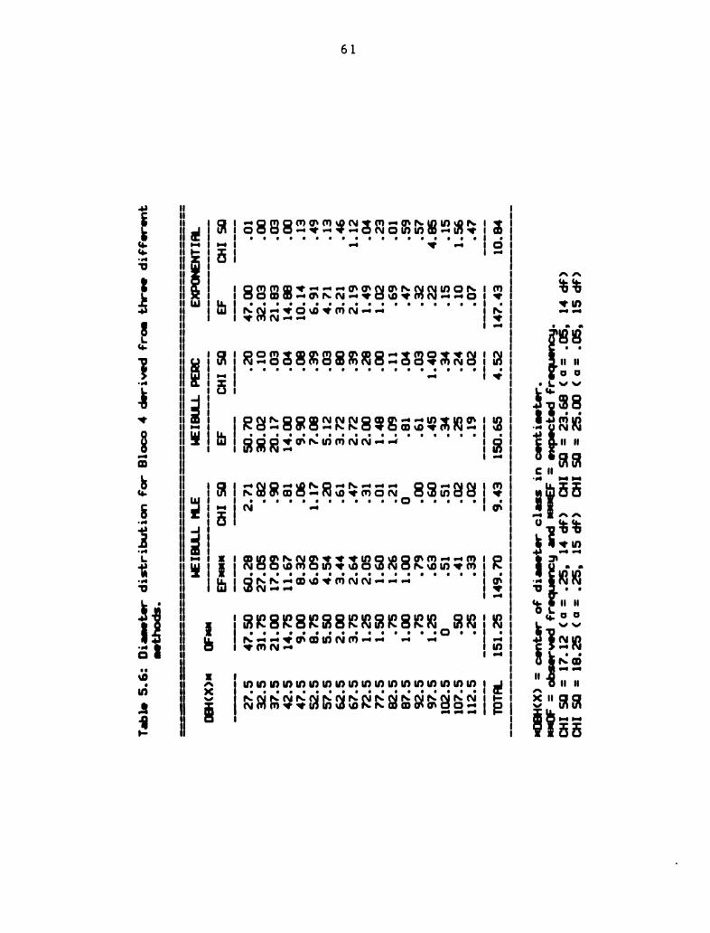
EXPCIENTIR.

Film

llE

metfods.

u-‘mm

UBH<X>I

Table

5.6:

Diameter

distribution

for

Bloco

4derived

from

three

different

my

Elm

PERC

EF

mmmmmmmemmumamaa mannaI. ...... cl" ..... «oh-mm

m“

“mammumnmww mnyawmwne

”maflmm&L&ZLL ....... mm

mmmwmmmfimwfiflmmmmwmmmnflm_ 1 “1

mmmmmmunnmmmmmmaawma.mmmuaz&1&&LL ...... “m

.mmmmmfiflmflflmmmomwflmmflem_2 1 .9

mmflmmflfim..flmm.mnam.a mE_wwwu864322L1L ..... &

.mnwnmnmmmamnwnaoma %

_manmamaaanh.n.n .. a

555£5£5£5fifififififijfifini

_aawenaweannmmuwmmm m

62

70-

{tree/ha

314

1L1

L1

13‘

N O

LL

Il

AL

L

..e

0 L4

.

A I

-..--___._V,,

10 20 30 40 50 50 70 80 90 100 110 120

DBH Gun)

PREDICTION BY WEIBULL MAX. UKEUHOOD

c211.

Figure 3.1: Becia 3 - The relationship between the observed

and estimated dbh frequencies, using the Heibull

HLE function.

Itroo/

r111

63

"5b"'eb"'7b” so so

DBH Own)

PREDICTION B'Y WEIBULL PERCENTILE

TM 110 120

Figure 5.2: Bacia 3 - The relationship between the observed

and estimated dbh frequencies, using the Heibull

PERC function.

ftree/ha

70-1

64

‘1'er VVY'VVV‘f' r'7111lvv'vrf

102030405000703'0901001101

DBH(cm)

PREDICTION BY EXPONENTIAL

Figure 5.3: Bacia 3 - The relationship between the observed

and estimated dbh frequencies, using the

Exponential function.

65

70

e m

a.o—eM

2 SD

\

g .. ."" so

3

ID

D

5......2,0 ..... 4'0.....i.....*mgh".¥b

DDH (cm)

(’0

§

.1“?

3 a can-usa can-us

fl-E Hm Ii!- “q HmI

2 “9 ad\ 3 g 3 .

g “5 2 “H L

‘Vwé ‘Kué

afiafi

0-3 01

40 I 1 20 40 u I 1

DB" (cm) . OBI-I (cm)

(a) (C)

Figure 5.4: Bloco l - The relationship between the observed

and the estieated dbh frequency distributions

by (A) Exponential, (B) Heibull PERC, and (C)

Heibull MLE functions.

66

:

- m

79.5O-e see-Its

”E

2 E\ a;

8 :

b{wj

- s

...;

aé

mi

113 -6IIIIIIgIIIII1%sssss3 iiiiiB'vagwsvvv‘k

DDH (cm)

(A)

‘H:

I “I“

mi

2 i

3 ”‘1of“?

3%

20-5

11.:

.3 '

40 I l

DBH(un)

Figure 5.5: Bloco 2 - The relationship between the observed

and the estimated dbh frequency distributions

by (A) Exponential, (B) Ueibull PERC, and (C)

Ueibull MLE functions.

67

70

e m

.0 v-e “I.“

2 SD

\

g 0

"3

ID

m ,

o .

N 1 1

DDI-I (cm)

(A)

70

a dame -.un—

fl' wwlfllun weaken

3‘” 3:»

\ \

9 ‘° 2in” In

w . 1 .

40 I l 40 u l 1

mfiIknd CBH(ufi)

(B) (C)

Figure 5.6: Bloco 4 - The relationship between the observed

and the estieated dbh frequency distributions

by (A) Exponential, (B) Heibull PERC, and (C)

Heibull "LE functions.

CHAPTER 6

A MARKOV CHAIN APPROACH TO PREDICT MORTALITY AND DIAMETER

DISTRIBUTION IN THE BRAZILIAN AMAZON.

6.1. INTRODUCTION

Little is known about forest structure and stand

dynamics of Amazonian tropical moist forests. Successive

records from representative long-term permanent plots

practically do not exist. The problem of reconstructing

forest history is greatly compounded by the fact that trees

can not be reliably aged, species diversity and spatial

heterogeneity are high, and fallen logs decay rapidly. It is

important to understand and report the natural changes that

occur in representative examples of pristine Amazonian

forests, because their composition and structure can be

altered by man as the demand for tropical timber species

increases.

The main objective of this chapter is to report S-year

changes in the overstory structure of an undisturbed

tropical moist forest. This will be done by the transition

probabilities of the overstory diameter distribution and

mortality of this forest, using a first-order Markov chain.

Diameter distribution and tree mortality will be projected

68

69

ahead to 1990 (t+2), based upon a 5-year period of

observations completed in 1985 (t+l) and its immediate past

in 1980 (t).

A first-order Markov chain is a stochastic process in

which the transition probabilities during the time interval

(t and t+l) depend only upon the state an individual is in

at time tior upon the knowledge of the immediate past at

til, not upon any previous state (Horn 1975, Chiang 1980,

and Bruner and Moser 1973). Shugart (1984) pointed out that

the time-invariant nature of each of the transition

probabilities is an important characteristic of the Markov

approach.

Shugart and West (1981) stressed that the importance of

understanding forest ecosystems is based not on their age,

but on known changes at present. Deterministic models

consisting of a single mathematical function (linear trend,

polynomial, sinusoids, or exponential growth or decay) have

not proven adequate when time series are involved (Morrison

1976).

In tropical moist forests, size may be more important

than age. One reason for this is that size may be more

ecologically informative than age when it is difficult to

make accurate estimates of age (Enright and Ogden 1979).

Division of life-cycles into developmental stages may allow

prediction of future behavior more accurately than division

into true age-classes. Usher (1966) used size attributes

instead of age to develop a model for the management of

70

renewable resources. He stressed that an organism which is

in i-th class at time t can be in the same class at time

£11, or it can be in a next class of that attribute, or it

can have died.

According to Enright and.Ogden (1979), the transition

matrix models in general are suitable for the analysis of

many biological problems, mainly in studies related to the

forest dynamics.

These models have been used intensively in studies of

dynamics of populations of plants or animals in many parts

of the world. Some examples are: the demography of jack-in-

the-pulpit in New York (Bierzychudek 1982); forest dynamics

of a population of Araucaria in a tropical rain forest in

Papua New Guinea, and Nothofagus in temperate montane forest

in New Zealand (Enright and Ogden 1979); termite succession

in Ghana (Usher 1979); forest succession in New Jersey (Horn

1975); the application, although without success. of this

model in secondary succession in coastal British Columbia

(Bellefleur 1981); the discussion of some extensions and

application of Hornfls Markov approach for forest dynamics in

tropical forests (Acevedo 1981); and the application of

Markov model to predict forest stand development (Usher

1966, Usher 1969, Bruner and Moser 1973, Peden et a1. 1973.

and Buogiorno and Michie 1980). Alder (1980) also described

the transition matrix as a possible tool for analysis of

growth and yield data for uneven aged mixed tropical

forests. Most of these works include a reasonable review

71

about the theory behind the Markov approach.<Grossman and

Turner (1974), Chiang (1980), and Anderson and Goodman

(1957) are very useful supplemental readings.

6.2. PROCEDURES

The data

The data for this study were collected on the research

area described in Chapter 4.

The Markov model

According to Bierzychudek (11982), a transition matrix

model is a size-classified model or a form of the Leslie

matrix model. The only requirement of this model is that the

population can be divisible into a set of states, and that

there exist probabilities for movement from one state to

another over time (Enright and Ogden 1979).

Here let the states be i, j = l, 2, .u., m. Let the

times of observation be t = 0, l, ...., T, and let Eli (t+1)

(i, j = 1, 2, ...., m) be the probability of state 1 at time

£11, given state i at time t.

A Markov process {X(t), t E [0,a>]} is said to be

homogenous with respect to time, or time homogenous. if the

transition probability

Pij(tvt+1) = Pr lX(t+1)=j|X(t)=il. i.j = 1, 2, ...., m.

72

depends only on the difference between t and t+1, but not on

t or t+l separately (Chiang 1980).

The computation of this probability can be done as

follows.

where: nij

First, calculate

Pij

given class i at time 3,

individuals in class i at time t.

= "ii/"i

and r1-

= number of individuals in class j.at time t+1,

= total number of

The transition probability matrix of a Markov chain for

a n-state process can be set up as:

j=l j=2 j=3 ..... J=m

r- “_I

1‘1 P11 P12 913 -°-°- Pim

i=2 P21 922 923 -°°-- sz

P = (pij) i=3 P31 P32 P33 °°°°° 93m

1:” Lfml sz pm3 "°°° pmm [ The probabilities Pij are nonnegative and the sum p11 + p12

+ pi3 + see Pim = 1a

The transition probability Pij can be of n-step

transition probability, pijI“). as the probability that the

population goes from state i on one trial to state i 3

trials later.1According to Bruner and Moser (1973), the n-

step transition probabilities matrix may be obtained by the

73

equation

PI“) = P“

where PI“) is the matrix of n-step transition probabilities

and Pn is the initial transition matrix raised to the n-th

power.

In this work, 15 states (i, j = l, 2, 3, u. 15) were

established as follow: state 1 = ingrowth (1), states 2 to

14 were defined as dbh classes, from 25 to the generalized

class next > 80 cm, in 5-cm interval, and state 15 =

mortality (M). Ingrowth is defined as those trees not tagged

in 1980 which in 1985 reached dbh >, 25 cm. The time interval

t and 511 are respectively, 1980 and 1985.

Tables 6.1, 6.2 and 6.3 present the transition of the

absolute frequency of individuals from the state i to state

1 during a 5-year period, respectively for bloco 1, bloco 2,

and bloco 4. The state ingrowth does not appear at time 1980

because it means only the movement to the higher dbh class

from the generalized dbh < 25 cm class.

The probability for transition among states was based

on the frequency of trees which either remained in the same

class, moved to a higher class, or died during a 5-year

period. Tables 6.4, 6.5 and 6.6 present the transitional

matrices for blocos 1, 2 and 4, respectively. These tables

were set up using their counterparts, Tables 6.1, 6.2 and

74

6.3, as bases for the computation of probabilities. For

example, the probabilities for the state 25 cm dbh class for

bloco 1 (Table 6.4) were calculated as follows: pq'z =

155/183 = 0.8470, 122,3 = 16/183 = 0.0874, and 112,15 = 12/183

= 0.0656. From all trees in 25 cm dbh class measured in

1980, 84.7% remained in the same class, 8.74% moved to the

30 cm dbh class, and 6.56% died during the period 1980-

1985. The probabilities for other dbh classes and blocks

were similarly determined with the respective counterpart

tables with absolute frequency distribution.

The tw0wstep transition matrix for each block (Tables

6.7, 6.8 and 6.9) were obtained by squaring their

counterparts (Tables 6.4, 6.5 and 6.6), respectively for

blocos l, 2 and 4. These tables represent the probability

for dbh and mortality distribution after two 5-year periods,

i.e., for t_+3, year 1990. The two-step transition matrix is

the basis for predicting the distribution of diameter and

mortality for the study area in 1990.

The eigenvalues (111-) of the transition matrix of each

sample plot were determined according to Anton (1973). The

dominant eigenvalue (Al = 1 since each matrix is non-

negative and row sums are 1) and the next largest modulus (

12) were determined. These values provide the ratio (Al/12)

which, according to Usher (1979), indicates the speed with

which the system will approach the ”climax" state.

75

6.3. DISCUSSION OF RESULTS

The projections for 1990 of number of survivors from

1980, the frequency distribution of dbh classes, and the

mortality by dbh classes, respectively for blocos 1, 2 and 4

are presented in Tables 6.10, 6.11 and 6.12. These

projections were determined based on the product of the two-

step transition matrix and the initial values of each state.

Volume stocking in 1990 can be estimated by applying a

reliable individual tree volume equation to the projected

diameter distributions. The frequency of individuals per dbh

classes is available for each sample plot.

The plot ratios (Al/A2) were 1.15, 1.00 and 1.00,

respectively for blocos 1, 2 and 4. The mean ratio, 1.05,

suggests that the studied area will approach the "climax"

state slower than the two systems discussed by Usher (1979),

mixed hardwoods in Connecticut (ratio 1.34) and in New

Jersey (ratio 1.57). This result makes sense if compared

with the distribution of changes in dbh classes and

mortality which occurred over a 5-year period. Using Table

6.13, which is the summary'of one-step transition matrix,

the mean estimates of the probability of changes and

mortality per plot are respectively 0.1205 and 0.0918. This

means that 12.05% of the total number of trees in a plot

changed dbh classes, and that 9.18% died during a 5-year

period. In an absolute basis, using the mean number of

trees/plot = 631, 76 trees changed classes, 58 died, and 23

(the mean ingrowth/plot) grew into the measurable dbh

76

classes. Thus, these results suggest that the studied area

is not a static population.

The projection for 1990, based on the summary presented

in Table 6.14, also does not show any trends that this

population is not changing. The average of the probability

of changes of dbh classes increased to 0.1895 and mortality

to 0.1717.

6.4. CONCLUSION

In the study area, the average rates of mortality and

ingrowth, during a 5-year period of observation, are

respectively 9.18% and 3.72% in relation to the total of

initial number of trees recorded in 1980.

There is no evidence that the probability of mortality

increases as dbh increase. The same trend is observed for

changes in dbh classes (the movement from one class to

another), i.e, the changes are occurring independently of

the diameter size.1As this study dealt with only the control

plots, it will be very interesting to compare these plots

with other experimental plots to see how effective were the

silvicultural treatments to change the rates of mortality

and ingrowth.

The ratio (Al/A2) leads to the conclusion that the

population under investigation is not static, that changes

are still taking place, and that the rates of ingrowth and

death are not perfectly balanced. However, it is also

77

necessary to keep in mind that this population is truncated

by size, i.e., only trees with dbh ; 25 cm were involved.

The Markov approach has a lot of potential. It can be

used as a baseline to project the mortality and diameter

distribution, or at least to predict the direction of future

trends, for forest management purposes in natural stands of

the Brazilian Amazon. It provides a general insight into the

nature of the dyamics of a sample of pristine Amazonian

forest which, consequently, will be very helpful to assist

decision makers in exploring and understanding the Amazonian

forest issues.

In 1990 this procedure will be repeated. Then, the

Markov chain approach will be evaluated and, if necessary,

refined based upon a 10-year of observatitun If valid, the

projection ahead to year 2000 will be possible.

Table

6.1:

Bloco

1-Transition

fromone

state

(i)

to

another

(j)

duringa

5-gear

period.

25

30

35

4D

45

50

55

6D

65

7D

75

>90newt

Htotal

0-0

“'3

26

26

155

16

12

193

109

27

17

153

52

22

1

45

4

33

wt

0'1

mvmm NNN d

"(Inn

11

2

“I“8889988882E§§:!

total

191

125

79

67

3B

31

29

13

ll

33

12

252

646

total/1990

=646

-l

(ingrowth)

=620

andtotal/1995

=646

-H

(mortalitg)

=594.

(I)

blank

spacesmean

zeros.

78

Table

6.2:

Bloco2

-Transition

fromonestate

(i)

to

another

(j)

tiringa

53-year

period.

jI

25

33

35

4D

45

50

55

6D

65

7D

75

>83next

Htotal

'd

20

172

20

122

23

112

87

13

7

46

16

8§§§88828**"*

“888998888288§:l

192

142

110

6D

62

25

19

17

65

24

45

i1

33

total/1m

=6m

-I

(ing’outh)

=668

andtotal/1%

=688

-H

(eortalitg)

=643.

(I)

blarkspacesmean

zeros.

79

Tdale

6.3:

Bloco4

-Transition

fromonestate

(i)

toanother

(j)

tiring

a5-gear

period.

Wmmmm

j125m§4045505560657075>mnextfltota1

an

24

24

15)

127

3$IIIIIIRI

NCJNQNWN-‘d

Q

91’

QIDIDWQn F.

N

II.

10an

ID

"namesamssetggglg

total/1m

=629

-I

(ingrowth)

=605

andtotal/1%!)

=629

-H

(mortalitg)

=567.

(it)bldk

spacesmean

zeros.

80

Tdale

6.4:

Dlooo

1-Transitionprobabilitgmatrix

fromone

state

(i)

toanther

(j)(bring

a5?.-

period.

ma—W

W***—M

j125

a)

54D

45

50

55

6D

65

7D

75

mnewt

I!

0‘

1.1111)

.9470

.CB74

(556

.7124

.1765

1111

.6667

.2921

.0129

035

.9333

.0741

.015

.0741

.7513

.11%

.154

0%9

.1667

.7692

.0769

15$

5!!!)

.7500

.25CIJ

.757

.1429

.0714

1

E

"8889988882883.

on

s-Ov-O

(in)blank

spacesmen

zeros.

81

82

.OOLONcoo.

IIOIQI

Jenna

any

aaao._

:

auuo..

axuc

oaaa._

aoA

aaao._

mu

comm.

comm.

an

aamw.

anon.

aamw.

mm

aamw.

cams

om

mo.~.

.mmo_.

wen»

mm

v_~o

man_

cams.

_am

mama.

mmno.

msua.

me

name.

mmmw.

mmnm.

av

vmma.

m.~..

_mdm.

mm

mane.

amen.

wmv_.

mass.

on.

nave

ammo.

m.mu.

mu

aaau..

um

zaxis

amA

ms

as

no

am

am

an

ac

av

an

an

m~

_n

.uomL-uL-cmumamcmgnu

Aw.

Luzaocno»

“my

.gnuu.cosaga

xmggncmum—«nunogu

camamncugp

uucoo—a

"m.uo—nup

83

60.30SeeI:

v1.325

oaaa._

:

noun."

axg:

__~_.

wmmo.

mmmm

aoA

anon.“

mu

acne.“

on

sumo.

same.

«man.

mu

am~..

omsm.

ow

mama.

mama.

~u_a.

mm

m~¢u.

smug.

v.n~.

om

wmma.

44mg.

cums

mv

mam".

mmm~

can“.

av

88.

:3.

~96.

mm

mvoo.

_mma.

tuna.

am

mm_~.

ages.

«mun.

am_a.

nu

ouao._

um

:ax.c

auA

mm

as

mm

um

mm

on

mv

av

mm

on

mw

na

.uowgonLucmrmamcmLau

any

Lasagna

0»

“my

canon

can«cum

xwgancmum—Mn-nogn:o.u.a¢og»

uvcacao

um.mo~nup

84

'30.»:Luau

eased;

)petq

(u)

0000'!

NW

9022'

8211'

8219'

2580'

665'

9295'

“2'

”16'

9260'

4169'

59m

9900'

5921'

5299'

W'

1110'

5512'

2191'

69(1'

6210'

[291'

9059

2692'

0110'

0921

2491'

81m'm'

6211'

9969'

M'

4900'

(580'

2829'

3999'

01.61

W'

590'

9892'

9218'

6121'

9310'

6%1'

9214'

9590'

9M'

0490'

~nameeamsaen§§=

0!.

aan."

oa<

94

oz

99

09

93

as

s»

or

as

as

92

1r

‘d4....-_.

...—.7.-WW+H4—H_.

...—4

'xsawtvfizstsq-qoaduoyzysUOJQ

6018-001CH1

-1

00013

=z'9

OIQIL

6.0:

Bloco

2-

111atin-steptransitionprobdailitg

eatrix.

1¢1e

an

540

45

50

55

60

j1a

.1

115111

oooooooooo

.238

.0260

.0015

.6611

.1010

.02“

.4577

.334

.

.7533

.7251

.1607

.0144

.mas

.53

.515

.09!)

ramsmamswamnmmn 00

blank

spaceseean

zeros.

Table

6.9:

Bloco

4-The

tun-step

transitionprobability

eatrix.

-....--mmm-m“...-“...“...mm

jI

25

30

35

40

45

50

55

60

65

70

75

>00

next

H

1.0150

.0632

.0053

.6655

.1150

.0123

.0004

.7144

.1124

.0097

.5311

.2005

.0264

.5625

.2950

.0167

.5951

.1362

.0070

.6695

.1539

.7656

.7512

.1245

1.0000

1.0000

.6944

.0463

.25

”WW"9:

mameeamaaargfx

l l.

(l)

blank

spaces

eean

zeros.

86

Table

6.10:

Bloco

1-Projection

For

1990.

eortalitg

dias.

distr.

survivors

0trees

m

in

1900

m

mu

13 6705 343 3

95m” .1

_nfiunwseaammmn

.

3463022201.

12

17

* mxnnmsumsaamn

m

.xamsmemsmemnmmu

102.10

543.02

_m

_m

...

z.

Tdale

6.11:

01oco2

-Projection

For

1990.

Otrees

din.

distr.

nrflwn:

nddfig 1

1g)

11'!

mm

”mauxmsnazmmm

”flaw-5461.1

%_ 02763240100011

l

_ .2..........m 0 7 64563L

1_ mmufi6all

% 20 076524

.. muuwgi

mgawmmaafifimmm

m wmxaaaaumzmnml 11

mammmmumamm341.

mmmmgawm441.

m _xamamam5wemnmmn_w

m.uwmgugmsmgmsmg1_mas

GENE

a.

MTU

m9§m0a§fl$fimw

t

.11

mgsn.mmnmummn_a

assaamewnummm

ammaaummuamaa

Issaastmgsuww

a99n63$9umm

mmmwaummwgwam

IaZOOIIZSZB‘Z

9mmwmwemeummu

g

I

,._m

m1

“3

“an.

”mums

wasp

"'19

Envy“

.mst

403mEWFO-‘d

-V00010'2‘?"Q"

90

in

1905.

bloco4

bloco2

bloco

1

1

Table

6.13:

Suseargof

one-step

transitionprobabilityeatrix

-

H

0656

1111

0305

0741

1364

0960

0

1667

1530

5000

0

0714

3

classes

'IGSIBS'QRIBSSRIQQ l '3“:

1&1e

6.14:

Sine-'9of

too-step

transition

probabilityaatrix

-projection

'88399883529 I"

l Ml?

.1339

.1970

.1477

.2497

.1749

.m

.3105

.0179

2.6626

.alg

91

CHAPTER 7

SHORT-TERM GROWTH OF UNDISTURBED BRAZILIAN AMAZON TROPICAL

MOIST FOREST OF "TERRA FIRME"

7 . 1 . INTRODUCTION

Based upon the available literature about growth and

yield studies, the mixed uneven-aged stands of the Amazonian

forest are condemned to stay where they have always been.

These forests are not an attractive forest investment

because little is known of the past growth and future growth

potential. Age and site index, two fundamental variables

used in developing even the simplest growth and yield models

(Sullivan and Clutter 1972, Ferguson and Leech 1978, Alder

1980, Smith 1983, and Clutter et al. 1983) are not

available. In addition, long-term successive measurements on

permanent sample plots are non-existent.

The main objective of this work is to give'a starting

point for growth and yield studies in the Brazilian Amazon

based on a 5-year period of observation. A major constraint

is that age, site index and total height of trees are not

available or even practical to obtain. Therefore, only

diameters measured in 1980 and their 5-year increments will

be used in an attempt to project growth and yield. Another

objective is to avoid the problems that the tropical

92

93

countries of southeast Asia have faced in terms of

divulgation of their experiences with growth and yield

studies. In Peninsular Malaysia, for example, although

growth and yield studies were established back in the

1950's, almost thirty years later few analyses have been

reported (Tang and Mohd 1981). Revilla (1981) also pointed

out that the growth and yield studies reported in Malaysia

and Philippines do not reflect the abundance of growth data

available.

7.2. PROCEDURES

This work focused on two separate aspects of growth and

yield, the current volume estimation for individual trees

and prediction of future volume.

In individual current volume estimation, the emphasis

was on the selection of the best model to estimate the 1980

and 1985 merchantable volumes based on either single-entry

(dbh as independent variable) or double-entry (dbh and

height as independent variables) regression equations. The

variable height (H) from double entry models was estimated

from diameter-height equations. Several regression equation

models were tested. The selection of the best model for

volume estimation was based on the Furnival index (Furnival

1961) - adjusted standard error of estimate (SEE) used to

compare logarithm equations with non-logarithm equations -

residual analysis and the coefficient of determination (R2).

In yield information and prediction, the emphasis was

94

on the development of individual volume growth models based

on diameter or basal area increments, the development of a

model for volume of 1985 as a function of the diameter or

volume measured in 1980, and the use of the exponential

Lotka's growth model for volume prediction on a hectare

basis.

The data

The data used to develop models for current individual

volume estimations came from Higuchi and Ramm (1985). For

this study, trees with dbh < 20 cm were excluded leaving a

total of 654 cases. Table 7.1 presents the basic

distributional characteristics of the data.

For yield information and prediction, the data came

from the three four-hectare permanent plots described in

detail in Chapter 4. I

The quantitative information for all three sample plots

are summarized in Table 7.3. These data refer to 52

botanical families found in the study area, including about

350 different tree species with dbh ; 25 cm. Three families

(Lecythidaceae, Leguminosae and Sapotaceae) contributed 50%

of the total number of trees. Table 7.4 presents the

distribution of frequencies of the three dominant families

in terms of status in 1980, mortality (M), ingrowth (I), and

various classes of periodic increment (PI).

95

Model development

From the available literature, models were selected

which matched the variables available for the study area.

For individual tree volume estimation, the following

models were tested:

(a) Single-entry models (Loetsch et al. 1973)

v = a + b*02 (1)

v = a + b*D + c*02 (2)

log V = a + b*log D (3)

log V = a + b*log D + c*(l/D) (4)

(b) Diameter/Height models

b*D + cm2 + d*D3 (Clutter 1963)+H=a

log H a + b*(l/D) (Loetsch et al. 1973)

l/H II

a:

+ b*(l/D) (Rai 1979) (7)

log H a + b*log D (Schreuder et al. 1979)

(c) Double-entry models (Loetsch et al. 1973)

log V = a + b*log D + c*log H or V = a*Db*H°

v = a + b*DZ*H (10)

For all models:

log denotes logarithm to base 10.

(5)

(5)

(8)

(9)

96

D denotes diameter at breast height (dbh) outside bark

in centimeters (cm). It is measured at 1.3 m above

ground level.

H denotes merchantable height in meters (m), i.e., the

length of stem from the ground to the crown.

V denotes merchantable volume in cubic meters (cu.m.).

For individual yield prediction, the following models

were tested:

(a) Increment

d0 = a + b*D + c*D2 (West 1980) (11)

dBA = a + b*D + c*02 (West 1980) (12)

d0 = a + b*(D - 25)2 (West 1981) (13)

Where: do = periodic diameter increment in cm.

dBA = periodic basal area increment in squared

meters (sq.m.).

These three models were weighted using the inverse of

the estimated sample variance as weight for each diameter

class. The weighted models will be equations (14), (15) and

(16).

(b) Volume in 1985 = f (1980 vol. or 1980 dbh)

V(85) a + b*D(80) + c*(D(80))2 (17)

0(85) a + b*D(80) (Soekotjo 1981) (18)

97

Where: V(85) = volume estimated in 1985 in cu.m.

0(85) dbh measured in 1985 in cm.

dbh measured in 1980 in cm.0(80)

(c) Lotka equation (Pielou 1977)

Adapting this model to predict volume growth produced

V(t) = V(0)*ert (19)

Where: V(t) = volume at time t (for t = l, 2, n 5-year

periods) in cu.m./ha.

V(0) = volume at time 0 (1980) in cu.m./ha.

r = b - d = the intrinsic rate of natural increase.

b= [I + Increment]/V(t) = ingrowth (I) and increment

rate (flow-in quantity).

d=M/V(t)= mortality (M) rate(flow-out quantity).

7.3. DISCUSSION OF RESULTS

Only 1/3 of the total of species belonging to the three

dominant families are considered commercial species by local

markets in Manaus. There exists no occurrence of the two

most valuable species for exportation of the Amazonian

forests, Swietenia macrophylla King (Mahogany) and Cedrela

odorata L"

The individual dbh periodic increment (PI) of the study

area averaged 1.06 cm, equivalent to 0.21 cm/year. This mean

P1 was estimated based on a population from which 31.3% did

98

not have any increment at all (Table 7.4). The mean dbh for

each increment class is also presented in Table 7.4. Note

that the maximum mean increment occurred in trees with 40.9

cm dbh, and that zero-increment occurred in trees with 42.5

cm dbh. More than 80% of trees had a PI less than 2 cm.

The average periodic annual increment (PAI), 0.21

cm/year, can be compared with the long-term PAI of 0.10 to

0.12 cm/yr obtained in Puerto Rico, Maricao and Luquillo

forests (Weaver 1982), and with the PAI of 0.22 to 0.48

cm/yr from the southern Ontario hardwood forest (West 1979).

The PAI for ”pau-rosa” (Aniba duckei Kostermans) at Ducke

Reserve, about 20 km north of Manaus, was 0.38 cm/year

(Alencar and Araujo 1981). In southeast Asia, however, the

dbh PAI's for virgin or managed forests are at least twice

as large as the PAI of the study area (Miller 1981 and Tang

and Mohd 1981).

Although the PAI is positive, the stand stocking

decreased during the period 1980-1985 in terms of number of

trees, basal area and volume (Table 7.3). This is explained

by a mortality rate which was twice the ingrowth rate.

Another explanation for the decreases is the mean dbh's for

mortality and ingrowth, which were 39 cm and 26.3 cm,

respectively (Table 7.3).

The regression models for individual trees volume

estimation were developed using the ordinary least squares

method. The regression summary for these models is presented

in Table 7.2.

99

The diameter/height models did not perform adequately

and, therefore, they were not used. Probably the reason for

failure in fitting the diameter/height curve is because

merchantable height was used instead of total height. All

proposed models used total height. In Rad's (1979) work, for

example, a R2 = 0.956 was obtained, while the highest R2 of

this work was 0.154.

To estimate the current volume of 1980 and 1985, the

following equation was used

log V = -3.4033 + 2.2673*log D (3)

This equation was chosen because it presented an appropriate

residual distribution, had an acceptable R2 and SEE, and

because it was as precise as the equation (4) with three

coefficients.

Before developing the proposed regression equations for

increment and growth' studies, a contingency table was

developed to test the differences in probabilities among

sample plots (Conover 1980).‘This test was carried out to

test the possibility of pooling the sample plots. In this

case let the probability of a randomly selected value from

the i-th bloco being classified in the j-th category be

denoted by Pij' for i = l, 2, 3, and j = l to 5.

The hypotheses were:

HO: All of the probabilities in the same sample plot are

equal to each other (i.e., plj = p2j = p3j for all j).

100

El: At least two of the probabilities in the same sample

plot are not equal to each other.

The chi-square test for differences in probabilities

was carried.out based on the tabulated data from Table 7.3

for number of trees and the mean diameter for each sample

plot. For contingency tables, the rows (j) were constituted

of different categories (status in 1980, status in 1985,

ingrowth, mortality, and periodic increment), and the

columns (i) by the sample plots (bloco l, bloco 2 and bloco

4). For both number of trees and mean diameter, the null

hypotheses could not be rejected. All sample plots were

combined therefore for further development of the growth and

yield models. .

All increment models developed had very poor fits, as

demonstrated by the low R2 values and high SBEs in Table

7.5. Model fit was not improved through the use of weighted

least squares. Based on these results S-year periodic

increments should not be used as a baseline for projection

of growth and yield of the Amazonian forests. A possible

explanation of this result is shown in Table 7.6a, which

contains the mean, standard deviation, minimum and maximum

increment.by dbh classes.‘The same procedure was used for

dbh when increment classes were considered (Table 7.6b). The

contingency table was used to test the differences in

probabilities for mean, standard deviation and maximum

increment and dbh. There were no differences among these

values for both diameter classes and increment classes.

101

Statistically, this means that the mean increment is not

significantly different between.dbh classes, and that the

mean dbh is equal for all increment classes.

In contrast, the two models, equations (17) and (18),

developed for individual volume and diameter growth

performed very well. The explanation for this successful fit

can be found in the explanation for the failure of increment

models. In model (16), for example, the objective was to

study the relationship between the dbh measured in 1985 and

the same dbh measured in 1980. As the increments were very

small, non-negative and non-significant, the dependent and

independent variables were approximately equal. In both

equations the regression coefficients were highly

significant. With these models one may now predict the

individual volume or dbh growth for another period of time,

for 1990, based on the dbh measured in 1985. In 1990, these

models can be validated and refined using, then, a lO-year

period.

Finally, fitting Lotka's model (19) to the data

produced

V(t) = v(o)*e(-0.0347*t)

The intrinsic rate of increase, r, was obtained on a

hectare basis based on the data from Table 7.3 as follows:

0' ll (3.8197 + 12.8010)/ 273.6415 = 0.0617

D: II 26.1019/273.6415 = 0.0954

102

r = 0.0617 - 0.0954 = - 0.0347

Using this equation, the estimated volume in 1985 is

V(1) = v(o)*e('0.0347*1)

V(1) = 274.7256 cu.m./ha

and for 1990

V(2) = V(0):e('0.0347*2)

V(2) = 265.3458 cu.m./ha

Based on the intrinsic rate of natural changes in a 5-

year period, the yield estimation for 1985 is very close to

the observed yield (V(85) = 273.642 cu.m). The projection

for 1990 also looks acceptable. This means that Lotkafis

model seems very promising to predict the future volume

yield. However, a longer period of observation is necessary

to fully validate this model.

7.4. CONCLUSION

In the study area the dbh increment for individual

trees during the period 1980-1985 averaged 1.06 cm. The

mortality rate was twice the ingrowth rate, and the stand

stocking decreased around 4% during this period.

Two models, V(85) = a + b*D(80) + c*(o(80))2 and

Lotka's model, could be used to estimate individual tree

volume for the next period with an acceptable reliability.

103

In 1990, then, these models can be retested, validated, and

refined, if necessary, using a lO-year period of

observation.

There was no indication that dbh could be used to

predict either the merchantable height or short-term

diameter/basal area increment.

Traditional growth and yield models can not be applied

to the Brazilian Amazon forests since age and site index are

not available. The only alternative remaining seems to be

the use of simpler models based on stand structure

monitoring at successive occasions.

The findings of this study suggest that the growth and

yield studies are not possible only on temperate forests,

but they are also feasible on an undisturbed tropical moist

forest in the Amazon. To achieve this goal, however, the

best estimation of the current volume and the dependability

of the permanent sample plots must be pursued.

T‘le

7.1:

Basic

distributional

characteristics

of

thedatamed

For

indivirhalvolmewion

equations

(pooled

data).

“I”

duh

(ca)

1.1951.

(a)

volume

(cu.m.

)

N

a 654

654

w

FEM

STEM.

HIN.

41.602

17.166

20.000

15.502

3.654

5.200

2.373

2.753

0.172

V

max.

120.!!!)

27.CID

27.”

104

Table

7.2:

Regression

summary

For

volume

estimation

mode1s1.

WWWW

600011005

ab

cd

0‘2

SEE

F1

(a)

Single-entry

U=

a+b0‘2

-0.3504

0.0013

0.90

0.0711

0.0711

9=

a+5

0+

c012

0.7353

-0.0451

0.0017

0.90

0.0504

0.0504

159u

=a

+b

1590

-3.4033

2.2573

0.92

0.1094

0.1729

109v

=a

+b

1090

+c

(170)

-2.5209

1.0390

-7.3077

0.92

0.1004

0.1714

(b)

Diameter/HeiQIt

logH

=a

+5

(1/0)

1.3009

-4.4002

0.15

0.0994

1.5152

1/H

=a

+b

(170)

0.0405

0.7133

0.13

0.0175

3.0007

logH

=a

+5

1590

0.7039

0.2492

0.14

0.1002

1.5204

H=

a+b

0+

cm2

400.3

4.7500

0.5015

-0.0057

0.0001

0.15

3.3512

3.3512 1002=

coefficient

of

determination,

SEE

=standard

error

of

estimate,

F1

=Furnival

index,

and

a,

b.

c,

andd

=regression

coefficients.

105

Table 7.3:

106

Characteristics of the data used as yield

information and for yield prediction.

STATUS # CASES MEAN TOTAL TOTAL

N dbh(cm) ba(sq.m.) vol(cu.m.)

BLOOD 1

1900 620 30.4 02.100 1165.974

1905 594 30.7 70.690 1111.470

Ingrowth 26 26.2 1.403 16.910

Mortality 52 41.3 0.507 127.000

P1 560 1.1 3.695 56.475

BLOCO 2

1900 667 36.7 77.060 1073.065

1905 642 37.3 77.300 1070.691

Ingrowth 20 26.6 1.109 13.421

Mortality 45 37.9 5.463 74.971

Pl 622 1.0 3.001 50.375

BLOCO 4

1900 605 30.0 02.210 1173.139

1905 567 39.1 70.163 1101.529

Ingrowth 24 26.1 1.200 15.506

Mortality 62 37.0 7.053 110.372

P1 543 1.0 2.517 30.762

MEANS

1900 631 30.0 00.726 1137.659

1905 601 30.4 70.056 1094.566

Ingrowth 23 26.3 1.267 15.279

Mortality 53 39.0 7.274 104.400

P1 570 1.0 3.330 51.204

MEANS/hectare

1900 150 20.102 204.415

1905 150 19.514 273.642

Ingrouth 6 0.317 3.020

Mortality 13 1.019 26.102

P1 145 0.034 12.001

P1 - Periodic increment a only trees measured in both

occasions, i.e., number of remaining trees in 1905 excluding

ingrowth which was not counted in 1900.

Tdale

7.4:

The

Frequencydistribution

of

the

three

dominantFailies

by

status

in

1%],

mortality

(M)

and

ing-outh

(1),

andbyperiodic

increment

(P1)

classes

in

cm.

WW.

P1=0

W1<1

1<P1<2

2<PI<3

3<Pl<4

Pl>4

116

92

FFHILIES

19m

fl

Lecythidaceae

347

19

75

Leg-inosae

333

Smtaceae

277

TOTE-3

Families

£7

76

61

203

212

00

91

59

70

41

13

19

77

_e—gne

.laezlsg:

227

29

TOTE-shale

area

1092

542

433

440

105

60

57

was)

42.5

33.6

35

5

107

108

[ID'O

9+32'

“(1'0

9+32'

100'0

0&0'11

CID'O

026'90

2(lJ'0

“9'9

9601

'1

9101'0

1100'1

0000'!

HID?

9201'1

(”3'0

9%1'1

066'0

366'0

91100

00000-

20000-

(“13'0-

ZEIII'D-

2%6'0

$20?-

IM'D-

KID'O

9910'0

1CD'0-

7000'0

9610'0

MW

0950

9046'0

19W'0-

0599'0

665'0

6903'0-

4275'0

(001%!

=(g)0

zvamamammw

=(QM)

‘1”

WHO-‘5

(9)

Zv(QZ-0)

9+

v=UP

240

9+

09

+t

=000

240

9+09

+t

=on

909961-H

<9)

zv(sz-a>

9+t

=on

290

9+09

+t

=HEP

2.0

9+09

+t

=0P

009951-n-uou

(r)

901MB

-s[apoeW

(:1)

p1.-

‘stapoe

sue-0401.11

pczubscn

(9)

‘stcpo-

1050.450;

powufisan-uou

(t)

493

9499-409188-4500

=9'201901

109

Table 7.6: Mean, standard deviation, minimum and maximum for

each (a) dbh classes and (b) increment classes.

(0) Periodic increment (PI) by dbh classes.

INCREMENT (cm)

DBH CLASSES(cm)

N MEAN STD.DEV. MIN MAX

25-29.9 531‘ 0.9177_ 0.9854 0.0 8.0

30-34.9 397 1.0091 1.1246 0.0 6.0

35-39.9 252 0.9274 1.1108 0.0 6.0

40-44.9 163 1.1313 1.2349 0.0 8.0

45-49.9 122 0.8852 0.9474 0.0 4.2

50-54.9 84 1.0964 1.3398 0.0 8.0

55-59.9 65 0.9862 1.4453 0.0 8.0

>60 119 0.7483 1.5173 0.0 7.2

overall 1733 0.9573 1.1400 0.0 8.0

(b) 00H by periodic increment (PI) classes.

00H (cm)

PI CLASSEStcm)

N MEAN STD.DEV. MIN MAX

0.0-0.49 672 40.6706 16.3201 25.0 116.0

0.5-0.99 303 33.7709 9.3157 25.0 92.0

1.0-1.49 312 35.5929 10.3603 25.0 94.0

1.5-1.99 136 35.6610 0.9577 25.0 62.0

2.0-2.49 130 30.4615 11.4764 25.0 76.0

2.5-2.99 55 39.0727 11.5002 25.0 73.0

>3.00 125 30.7200 12.7459 25.0 91.0

overall 1733 37.0697 13.5655 25.0 116.0

CHAPTER 8

CONCLUSIONS

The forest resources of the study area are declining

with respect to number of trees per unit area, growing stock

volume and basal area.

The dominant latent root, A.= 0.97, supports the

previous affirmation. According to Enright and Ogden (1979).

when the intrinsic rate of natural increase (r) is equal to

zero, A is equal 1, i.e., the population under investigation

is perfectly balanced or the birth rate is equal to the

mortality rate; when r > 0, A > 1, the population is

increasing and the birth rate is greater than the mortality

rate; and when r < 0, A < l, the population is declining

or the birth rate is smaller than the mortality rate.

Another reason for the decline is that mortality and

ingrowth are not balanced.'These components averaged, during

a 5-year period of observations, 9.18% and 3.72%

respectively, in relation to the total recorded in 1980.

Mortality appears to be independent of diameter size.

However, the survivors are growing at a mean rate of 0.21

cm/year in dbh.

The ratio Al/Az averaged 1.05, suggesting that this

population will approach the ”climax” state slower than at

110

111

least two mixed temperate hardwood systems, one in

Connecticut and another in New Jersey.

In terms of utilizable volume stock, the forest of the

study area,(control plots of NR experiment) is relatively

poor. The total volume including bark averaged 284 cu.m/ha

for all tree species with dbh >, 25 cm. From this total, only

about 40% fulfills the minimum size requirements (dbh > 40

cm) for Amazonian forest industries, and from this only

about 30% qualifies as economically desirable species. Thus,

the remaining utilizable volume is no more than 35 cu.m/ha.

This is much less than half of the average volume reported

for growing stock of North American temperate forests,

Brazilian temperate forests, or even tropical moist forests

in SE Asia.

In contrast, the area is very important in species

richness. About 350 different tree species from 52 different

botanical families were identified. Lecythidaceae,

Leguminosae and Sapotaceae are the dominant families

contributing more than 50% of all trees tallied.

Among the three hypothesized diameter distribution

functions tested in this study, the Weibull PERC

(distribution whose parameters were computed using the

percentile approach) showed the best fit for the observed

data. The Weibull MLE (the maximum likelihood approach) and

the exponential distributions were very sensitive to

variation within sample plots. When the Weibull shape

parameter, 0, equals 1, an exponential distribution results,

112

but even in this case, the Weibull PERC fitted the observed

data as precisely as the exponential function. In addition,

the Weibull PERC function is very simple in estimating its

parameters; it does not require sophisticated computer

capabilities.

The first-order Markov chain analysis allowed

projection of the overstory mortality and frequency

distribution by dbh classes. Since age and successive

records from long-term permanent plots are not available,

the Markov approach is a realistic alternative to predict

the direction of future trends in the study area.

Traditional growth and yield models cannot be applied

to the study area since age and site index are not

available. The 5-year increments did not show any

indications that they can be correlated with dbh. From this

study, Lotka's model appears to be a powerful alternative to

replace the traditional growth and yield models. Another

alternative is the equation, V(85) = a + b* 0(80) +

c*(D(80)f2, which presented a very good fit for the observed

data.

All mathematical models developed in this study have as

output the abstract model for a management strategy to be

implemented in the real world. In 1990, these models should

validated and, if necessary, refined based then on a 10-year

period of observations. If valid, they will be very helpful

to exercise the simulation as a means of determining model

time response for a longer period.

APPENDIX

APPENDIX

Floristic composition of bacia 3 by botanical family

(Developed by Department of Botany of INPA)

1. ANACARDIACEAE

Anacardium spruceanum Benth ex Engl.

Astronium - l sni(*)

Tapira retusa Ducke

2. ANONACEAE

Anaxagorea - l sni

Anona ambota Aubl.

Bocageopsxs multiflora (Mart.) R.E. Fr.

Bocageopsis - l sni

nguetia flagelaris Huber

Duguetia - l sni

Ephe ranthus amazonicus R.E. Fries

Ephedranthus - l sni

Quatteria olivacea R.E. Fries

Guatteria - l sni

gseudoxandra cariaceae R.E. Fries

Bollinia insignia R.E. Fries var. pallida R.E. Fries

Unono sis - l sni

Xylopia benthami R.E. Fries

Xylopia - l sni

3 . APOCYNACEAE

Ambelania acida Aubl.

Anacampta - l sni

Aspidosperma album (Vahl.) R. Ben.

Aspidosperma obscurinervius Azamb.

AspidOsperma carapanauba Pichon

Aspidosperma - l sni

gouma macrocarpa Barb. Rodr.

geissospermum ar enteum R. Rodr.

Himatanthus sucqua (Spruce) Woodson

4. ARALIACEAE

Didymopanax morototoni (Aubl.) Decne. & Planch.

* sni = species not identified for determined genus.

113

9.

114

BOMBACACEAE

Bombacopsis - 2 sni's

gatostemma milanezii Paula Nov.

§cleronema micranthum Ducke

Scleronema - l sni

BIGNONIACEAE

Jacaranda copaia D. Don.

Jacaranda - l sni

Tabebuia serratifolia (D. Don.) Nichols.

BORAGINACEAE

Cordia - 1 sni

BURSERACEAE

gemicrepidospermum rhoifolium (Bth.) Swart.

grotium aracouchili (Aubl.) March.

grotium heptaphyllum (Aubl.) March.

grotium subserratum Engler

Protium - 4 sni's

Tetra astris unifoliata (Engl.) Cuatr.

Tetragastris - 2 snI's

Trattinickia - l sni

CARYOCARACEAE

garygcar pallidum A.C. Smith

Caryocar villosum (Aubl.) Pers.

10L CELASTRACEAE

Goupia glabra Aubl.

11. CHRYSOBALANACEAE

gouepia leptostachya Benth. ex Hook

Coue ia - l sni

Birtella glandulosa Spreng.

Licania a1 a (Ben.) Cuatr.

canescens R. Ben.

Licania

Licania

Licania

Licania

fiicania

Licania

Licania

Eicania

Licania

Licania

gracilipes Taub.

heteromorphg

hypoleuca Benth.

kunthiana Hook f.

latifolia Benth. ex Hook

micrantha Miq.

oblongifalia Standl.

reticulata Prance

- l sni

Parinari montana Aubl.

12. COMBRETACEAE

Buchenavia parvifolia Ducke

Buchenavia - 2 sni s

13.

14.

15.

16.

17.

18.

19.

20.

115

CONNARACEAE

Connarus - l sni

DICBAPETALACEAE

Tapura amazonica

DUCKEODENDRACEAE

Duckeodendron cestroides Ruhlm

EBENACEAE

Diospyros bullata A.C. Smith

ELAEOCARPACEAE

Sloanea - l sni

ERYTHROXYLACEAE

Erythroxylum - lsni

EUPHORBIACEAE

Anomalocalyx - l sni

Qpnceveiba guianensis Aubl.

Qroton lanjouwensis Jablonski

Croton - l sni

erpetes variabilis Vittien

Qavarretia - 1 sni

glycidendron amazonicum Ducke

Hevea guianensis Aubl.

Mabea caudata Pax. ex K. Holhm.

Mabea - l sni

Micrandra rossiana R.E. Schultes

Micrandra siphonioides Bth.

Micrandropsis scleroxylon W. Rodr.

gausandra macropetala Ducke

Pera - 1 sni

ngonophora schomburgkiana Miers. ex Bth.

FLACOURTIACEAE

gasearia combaymensig Tul.

gasearia ulmifolia Vahl. ex Von.

Casearia - l sni

Carpotroche - l sni

Laetia procera (Poepp.) Eichl.____,_

Ryania - l sni

21. GUTTIFERAE

Qalophyllum brasiliense Camb.

Carai a - l sni

Clusia - l sni

Havetiopsis - l sni

Moronobea coccinea Aubl.

Moronobea pulchra Ducke

Rheedia 2 - sni‘s

Symphonia globulifera Linn

V smia uckei Maguire

22.

23.

24.

25.

116

Vismia guianensis (Aubl. ) Choisy

Tovomita - l sni

HIPPOCRATEACEAE

Salacia - l sni

HUMIRIACEAE

Duckesia verrucosa (Ducke) Cuatr.

Endopleura uchi (Huber) Cuatr.

Humiria balsam1fera (Aubl. ) St. Hill

Sacoglottis ceratocarpa Ducke

Sacaglott1s - l sni

Vantanea macrocarpa Ducke

Vantanea parviflora Lam.

Vantanea - l sni

ICACINACEAE

Emmotum - 2 sni's

Poraqueiba - l sni

LAURACEAE

Aniba canelilla (B. B. K. ) Mez.

Aniba duckei Kosterm.

Aniba ferrea Kubitzki

Aniba rosaedora Ducke

Aniba terminalis Ducke

Aniba - l sni

Endlicheria - 4 sni's

Licaria canela (Meissn. ) Kosterm.

Licaria guianensis Aublet

Licaria rigida Kost.

Licaria - 3 sni' s

Mezilaurus decurrens (Ducke) Kost.

Mezilaurus synandra (Mez.) Kosterm.

Mezilaurus - l sni

Nectandra rubra (Mez.) C.K. Allen

Nectandra - l sni

Qcotea canaliculata Mez.

Ocotea neesiana (Miq.) Kosterm.

Ocotea - 9 sni's

26. LECYTHIDACEAE

Cariniana decandra Ducke

Car1niana micrantha Ducke

Corytophora alta Knuth

Corytophora rimosa Rodr.

Couratari - l sni

_schweiIera fracta R. Knuth

§schweilera odora (Poepp.) Miers.

Eschweilera - 8 sni's

Gustavia au usta L.

GustavIa elliptica Mori

Holopyx1dium latifolium (A. c. Smith) R. Knuth.

Lecythis usitata Miers var. paraensis R. Knuth.

117

27. LEGUMINOSAE CAESALPINIODEAE

Aldina hetero h lla Spruce ex Bth.

Bocoa viridirora (Ducke) Cowan

Cassia rubriflora Ducke

Copaifera multijug_ Hayne

Elizabetha bicolor Ducke

Elizabetha princeps Schomb. ex Bth.

Elizabetha - l sni

Eperua bijug_ Mart. ex Benth. var. glabriflora Ducke

§pgrua duckeana Cowan

Eperua schomburgkiana Benth.

Hymenaea pArvifolia Huber

Hymenaea - 4 sni' s

Macrolobium limbatum Spr. ex Benth.

Macrolobium microcalyx Ducke

Peltogyne cat1nggg subsp. labra (W. Rodr. ) M. F.Silva

Peltogyne paniculata subsp. pAniculata Benth.

Swartzia ingifolia Ducke

Swartzia pgnacoco (Aubl. ) Cowan

§wartzia polyphyl1g D.C.

§wartz1a recurva Poepp. & Endl.

Swartzia reticglata Ducke

Swartzia ulei Harms

Swartzia - 3 sni's

§g1erolobium - l sni

Vouacapoua pallidior Ducke

Tachigalia myrmecophilla (Ducke) Ducke

TAch1gAl1a pAn1culata Aubl.

Tach1gA11a - l sni

28. LEGUMINOSAE MIMOSOIDEAE

Dimorphandra parviflora Spr. ex Bth.

Diniz1a excelsa Ducke

Enterolobium schomburgkii Benth.

Hymenolobium - l sni

Inga aff. brevialata Ducke

Inga paraensis Ducke

Inga cayennensis Benth.

Inga - 4 sn1' s

Parkia multiju a Bth.

Parkia opposit olia Spr. ex Bth.

Parkia pendula Benth. ex Walp.

Parkia - 2 sn '3

Piptadenia psilostachya (D. C. ) Bth.

Piptaden1a suaveolens Miq.

g1ptadenia - 1 sni

Eithecolobium racemosum Ducke

Pithecolobium - 2 sni‘s

Sgryphnodendron racemiferum (Ducke) W. Rodr.

Stryphnodendron - l sni

29. LEGUMINOSAE PAPILIONOIDEAE

Andira parviflora Ducke

30.

31.

32.

33.

34.

118

Andira unifoliata Ducke

Andira - l sni

DIpteryx alata Vogel

Dipteryx ma nifica Ducke

Dipteryx odorata (Aubl. ) Willd.

DApteryx oppositifolia (Aubl. ) Willd.

Dipteryx polyphylla (Ducke) Hub.

fiipteryx - 1 sni

gymenolobium sericeum Ducke

gymenolobium cf. pulcherrimum Ducke

gymenolobium - l sni

Ormosia sm1thii Rudd.

Diplotrop1s - l sni

Platymiscium duckei Huber

LINACEAE

Roucheria callophylla Planch

MALPIGHIACEAE

gyrsonima stipulacea Adr. Juss.

B rsonima - l sni

Pterandra arborea Ducke

MELASTOMATACEAE

Bellucia grossularioides (L. ) Triana

Miconia elaeagnoides Cogn.

Micon1a re e111 Cogn.

Mouriria angulicosta Morley

MourirIa - l sn1

MELIACEAE

Guarea - 2 sni's

Trichilia - 2 sni's-

MORACEAE

Brosimum guianensis Aubl.

Brosimum pgtabile Ducke

Brosimum pgr1nar1oides Ducke subsp. parinarioides

Brosimum utile (H. B. K. ) Pittier

Brosimu rubescens Taub.

Cecropia scyadophylla Mart. var. juranyana Snethlage

Claris1a racemosa R.et P.

Cousapoua - 1 sni

Pcus clusiaefolia Schott

F1cus guianensis Desv.

HelicostyAis - l sni

Maggira calophylla (P.A.E.) C.C. Berg.

Magu1ra sclerophylla (Ducke) C. C. Berg.

NaucleOpsis caloneura (Hub. ) Ducke

Naucleopsis glabra Spruce ex Baill

Naucleopsis macrophylla Miq.

Perebea mollis (P. E. ) Huber subsp. mollis

Perebea mollis (P. S. C. ) Huber

Pourouma ovata Trecul.

35.

36.

37.

38.

39.

40.

41.

42.

43.

44.

119

Pseudolmedia - 1 sni

Sorocea - 1 sni

MYRISTICACEAE

gpgpsoneura ulei Warb.

lryanthera - 1 sni

Osteophloeum lat s ermum (A.D.C.) warb.

Virola calophylla Mgf.

girola carinata (Bth.) Warb.

ViroIa elon ata (Bth.) Warb.

Virola c . m1chelii Beckel

girola multinervia Ducke

girola pavonis (A.D.C.) Smith

girola venosa Warb.

Virola venosa (Benth.) Warb.

MYRTACEAE

Eu enia - 3 sni's

M rc1a ma na Legrand

Mxrc1a a ax (Rich.) D.C.

MONIMIACEAE

Siparuna dicipiens (Tu1.) A.D.C.

NYCTAGINACEAE

Neea cf. altissima P. et E.

Neea - 2 sni‘s

OCHNACEAE

Ouratea discophora Ducke

Ouratea - 1 sni

OLACACEAE

Agtandra - 1 ani

Qhaunochiton - 2 sni's

Beisteria acumitetg (B.B.) Engl.

BEISteria barbata Cuatr. .

Beisteria - 2 sni's

ginquartia guianensis Aubl.

Ptychopetalum olacoides Benth.

PROTEACEAE

Rougala - 1 sni

QUIINACEAE

Quiina abovata Tul.

Quiina - 1 sni

Touro ia guianensis Aubl.

RHABDENDRACEAE

Rhabdodendron amazonicum (Spr. ex Bth.) Bub.

RBIZOPHORACEAE

Anisophyllea manausensis Pirea 5 W. Rodr.

120

Sterigmapetalum obovatum Kuhlmann

4S. RUBIACEAE

Amaioua - 1 sni

Duroia fusifera Hook f. ex K. Schum

Duroia - 1 sni

Elaeagia - 1 sni

Faramea - 1 sni

Perainandusa - 2 sni' s

PTlicourea anisoloba M. Arg.

Palicourea cf. leggiflora (Aubl. ) A. Rich.

PTgamea - 1 sni

Psychotria prancei Steyermark

Remijia - 3 sni' s

46. SAPINDACEAE

Mata ba - 1 sni

M1cropholis - 1 sni

Talis1a - 1 sni

Toulicia - 1 ani

47. SAPOTACEAE

Achrouteria Egmifera Eyma

Achrouter1a - 2 sn1 s

Chrysophyllum oppositum (Ducke) Ducke

Chrysophyllum anomalum Piree

Diplocem venezuelana Aubr.

Ecclinusa Bacuri AfiBr. et Pellegr.

Ecclinusa ucugu1rana Aubr. 5 Pellegr.

Ecclinusa - 2 sn1 s

Pranchetella platyphylla (A. C. Sm.) Aubr.

Pranchetella - 1 sni

Glycoxylon pedicellatum (Ducke) Ducke

Lafiétia - 4 sni' s

Manilkara amazonica (Huber) Standley

Manilkara huberi (Ducke) Chev.

Manilkara cavalcantei Pires et Rodr.

Manilkara surinamenEis (Miq.) Dubard

Micropholis truncifiora Ducke

Micropholis guyanensis Pierre

Micropholis venulosa Pierre

Micropholis rosaainha-brava Aubr. et Pellegr.

Microphol1s mensalis (BTehni) Aubr.

Microphol1s - S sni' s

Myrtiluma eu eniifolia (Pierre) Baill

Neoxxthecec uaantha (Sandw.) Aubr.

Pouteria ggyanensis Aubl. L. O.A. Teixeira 82

Pradosia verticillata Ducke

gr1eure11a manaosens1s Aubr.

Pseudolabatié - 1 sni

RafilkoEerelIa - 1 sni

Ra ala spuria (Ducke) Aubr.

R1charde11a manaosensis Aubr. et Pellegr.

Richardella macrophylla (Lum.) Aubr.

48.

49.

SO.

51.

52.

'53.

54.

121

szxgiopsis oppositifolia Ducke

SarcauIis brasiliensis (A.D.C.) Eyma

SIHARUBACEAE

§imaruba amara Aubl.

Simaba guianensis Aubl. subsp. guianensis

SImaEa cuspidata Spruce

STERCULIACEAE

§terculia speciosa K. Schum.

Sterculia - 1 sni

TheoEroma sylvestris Aubl. ex Mart.

STYRACACEAE

Stxrax - 1 sni

TILIACEAE

Apeiba echinata Gaertn.

Apeiba burchelii Sprague

Luehea - 1 ani

VERBENACEAE

Vitex triflora Vahl.

VIOLACEAE

geonia glycicarpa Ruiz et Pav.

ginorea guianensis Aubl. var. subintegrifolia

Rinorea racemosa (Mart. et Zucc.) O. Ktze.

égphirshox sufihamensis Eichl.

VOCHYSIACEAE

Erisma bicolor Ducke

Erisma fuscum Ducke

Qualea clavata Staflen

Qualea paraensis Ducke

QuaIea cassiquiarensig (Spr.) Warm.

Qgglea labourianana Paula

nglea brevipediceilata Staflen

Vochysia obiflénsis (355.) Ducke

LIST 01? REFERENCES

LIST OF REFERENCES

Acevedo, M.F. 1981. On Born's Markovian Model of Forest

Dynamics With Particular Reference to Tropical

Forests. Theoretical Population Biology 19:230-250.

Alder, D. 1979. A Distance-independent Tree Model for

Exotic Conifer Plantations in East Africa. Forest Sci.

25:59-71.

Alder, D. 1980. Forest Volume Estimation and Yield

Prediction. Vt2 - Yield Prediction. FAD Forestry Paper

22/2. 194p.

Alencar, ch. and qu. Araujo. 1981. Incremento Anual do

Pau-rosa (Aniba duckei Kostermans) Lauraceae, em

Floresta Tropical Umida Primaria. Acta Amazonica

11(3):547-552.

Anderson, T.W. and INA. Goodman. 1957. Statistical

Inference About Markov Chains. Annals of Mathematical

Statistics 28:89-110.

Anton, B. 1973. Elementary Linear Algebra. John Wiley and

Sons, Inc. New York. 296p.

Bailey, R.L. and T.R. Dell. 1973. Quantifying Diameter

Distributions With the Weibull Function. Forest Sci.

19:97-104.

Barros, P.L.C., S.A. Machado, D. Burger, and J.D.P.

Siqueira. 1979. Comparacao de Modelos Descritivos da

Distribuicao Diametrica em uma Floresta Tropical.

Floresta lO(2):l9-32.

Bell, 6.8. 1976. Notes on Natural Regeneration in Dominica.

Windward Islands. Commonw. For. Rev. 55(l)27-36.

Bellefleur, P. 1981. Markov Models of Forest-type Secondary

Succession in Coastal British Columbia. Can. J. For.

RES. 11:18-29.

Bierzychudek, P. 1982. The Demography of Jack-in-the-

pulpit, a Forest Perennial That Changes Sex. Ecol.

Monographs 52(4)::335-351.

Braga, IhI.S. 1979. Subdivisao Fitogeografica, Tipos de

Vegetacao, Conservacao e Inventario Floristico da

122

123

Floresta Amazonica. Acta Amazonica 9(4):53-80.

Britwum, S.P.K. 1976. Natural and Artificial Regeneration

Practices in the High Forest of Ghana. Ghana Forestry

Journal 2:45-49.

Bruner, 3.0. and J.W. Moser Jr. 1973. A Markov Chain

Approach to the Prediction of Diameter Distributions

in Uneven-aged Forest Stands. Can. J. For. Res. :409-

417.

Brunig, E.F. 1977. The Tropical Rain Forest - A Wasted

Asset or an Essential Biosphere Resource? Ambio 6(4).

Budowski, G. 1976a. Why Save Tropical Rain Forests? Some

Arguments for Campaigning Conservationists. Amazoniana

5(4):529-538.

Budowski, G. 1976b. Los recursos naturales en el desarrolo

del Tropico Bumedo. Reunion sobre desarrolo regional

del Tropico Americano. IICA-Tropicos. Belem, Para,

Brazil.

Buogiorno, J. and B.C. Michie. 1980. A Matrix Model of

Uneven-Aged Forest Management. Forest Sci. 26:609-625.

Chai, D.N.P. and M.P. Udarbp. 1977. The Effectiveness of

Current Silvicultural Practice in Sabah. The Malaysian

Forester 40(1):27-35.

Cheah, INC. 1978. Forest regeneration and development

options in Peninsular Malaysia today. The Malaysian

Forester 41(2):17l-l75.

Chiang, CAL. 1980. An Introduction to Stochastic Processes

and Their Applications. Robert E. Krieger Publ. Co.

Huntington, New York.

Clutter, £LL. 1963. Compatible Growth and Yield Models for

Loblolly Pine. Forest Sci. 9:354-371.

Clutter, J.L., J.C. Fortson, L.V. Pienaar, G.B. Brister,

and R.L. Bailey. 1983. Timber Management: A

Quantitative Approach. John Wiley and Sons, Inc. New

York. 333p.

Cochrane, T.T. and P.A. Sanchez. 1980. Land Resources,

Soils and Their Management in the Amazon Region: A

State of Knowledge Report. In: Amazonia - Agriculture

and Land Use Research - proceedings of the

International Conference at CIAT in Cali, Colombia.

Cohen, AnC. 1965. Maximum Likelihood Estimation in the

124

Weibull Distribution Based on Complete and on Censored

Samples. Technometrics 7(4):579-588.

Conover, WuJ. 1980. Practical Nonparametric Statistics.

John Wiley and Sons, Inc. New York. 2ed. 493p.

De Graaf, N.R. 1981. Sustained Timber Production in the

South American Tropical Rainforest. Paper prepared for

the workshop on Management of low fertility acid soils

of the Humid American Tropics in Paramaribo. (copy).

Departamento de Silvicultura Tropical. 1982. Inventario

Florestal no Rio Trombetas (INPA/SBELL/ALCOA).

Technical Report. 49p.

Departamento de Silvicultura Tropical. 1983. Inventario

Florestal da UBE de Santa Izabel. Technical Report.

35p.

Departamento de Silvicultura Tropical. 1983. Inventario

Florestal do Projeto Rio Arinos. Technical Report.

64p.

Departamento de Silvicultura Tropical. 1983. Inventario

Florestal da UBE de Balbina. Technical Report. 111p.

Draper, NzR. and B. Smith. 1981. Applied Regression

Analysis. John Wiley and Sons, Inc. New York. 2ed.

709p.

Einsesmith, S.P. 1985. PLOTIT: User's Guide.

Enright, N. and J. Ogden. 1979. Applications of Transition

Matrix Models in Forest Dynamics: Araucaria in Papua

New Guinea and Nothofa us in New ZeTland. Australian

Journal of Ecology 4:3-g3.

Ferguson, I.S. and J3W. Leech. 1978. Generalized Least

Squares Estimation of Yield Functions. Forest Sci. 24:

27-42.

Fox, J.E.D. 1976. Constraints on the natural regeneration

of tropical moist forest. Forest Ecology Management

1:37-65.

FUA - Fundacao Universidade do Amazonas. 1979. Proposta de

Politica Florestal para a Amazonia Brasileira. Metro

Cubico - Livros e Revistas Tecnicas Ltda. Manaus, Am.

72p.

Furnival, G.M. 1961. An Index for Comparing Equations Used

in Constructing Volume Tables. Forest Sci. 7:337-361.

Gomez-Pompa, A., c. Vazquez-Yanes, and S. Guevara. 1972.

125

The Tropical Rain Forest: A Nonrenewable Resource.

Science 177:762-765.

Grossman, 8.1. and J.E. Turner. 1974. Mathematics for the

Biological Sciences. Macmillan Publishing Co., Inc.

New York. 512p.

Higuchi, N. 1981a. A silvicultura no INPA. Supl. Acta

Amazonica 11(1):99-107.

Higuchi, N. 1981b. Relatorio sobre o Encontro da IUFRO nas

Filipinas e ”study-tour” por Filipinas, Sarawak e

Fiji. Report not published.

Higuchi, N., F.C.S. Jardim, J. Santos, A.P. Barbosa, and

T.W.W. Wood. 1983. Inventario Florestal Comercial da

Bacia 3. Acta Amazonica (in press).

Higuchi, N., F.C.S. Jardim, J.Santos, and J.C. Alencar.

1985. Bacia 3 - Inventario Diagnostico da Regeneracao

Natural. Acta Amazonica 15(1-2):199-233.

Higuchi, N. and C.W. Ramm. 1985. Developing Bole Wood

Volume Equations for a Group of Tree Species of

Central Amazon (Brazil). Commonw. For. Rev. 64(1):33-

41.

Hilton, R.G.B. and R.J. Johns. 1984. The future of forestry

in Papua New Guinea. Commonw. For. Rev. 63(2):103-106.

Horn, H.S. 1975. Markovian Properties of Forest Succession.

In: Ecology and Evolution of Communities (M. Cody and

J. Diamond, eds.) pp. 196-211. Harvard University

Press. Cambridge, Mass.

Hosokawa, R.T. 1981. Manejo de Florestas Tropicais Umidas

em Regime de Rendimento Sustentado. UFPr. Technical

Report.

Hutchinson, I.D. 1980. Liberation Thinning: A Tool in the

Management of Mixed Dipterocarp Forest in Sarawak.

UNDP/FAO Field Document 8 5. Kuching.

IBGE. 1977. Geografia do Brasil. Sergraf—IBGE. Vol. 1 and

4.

INPA - Instituto Nacional de Pesquisas na Amazonia. 1979.

Estrategias Para a Politica Florestal na Amazonia

Brasileira. Suplemento Acta Amazonica 9(4). 216p.

INPA - Instituto Nacional de Pesquisas na Amazonia. 1982.

Bacia Modelo: Caracterizacao Ecologica de uma Bacia

Hidrografica Experimental na Amazonia Central.

Suplemento Acta Amazonica 12(3). 114p.

126

James, L.M. (pers. comm.). Notes of FOR 454 - Forestry in

International Development. Winter/1984.

Johnson, N.E. 1976. Biological opportunities and risks

associated with fast-growing plantation in the

Tropics. Journal of Forestry, Apri1:206-211.

Kio, P.R.o. 1976. What future for natural regeneration

of tropical high forest? An appraisal with examples

from Nigeria and Uganda. Commonwealth Forestry Review

55(4):309-318.

Kio, P.R.O. 1979. Management Strategies in the Natural

Tropical High Forest. Forest Ecology and Management

2:207-220.

Lanly, J.P. 1983. Assessment of the Forest Resources of the

Tropics. Forestry Abstracts (Review Article) 44(6):287-

318.

Lawrence, K.D. and D.R. Shier. 1981. A Comparison of Least

Squares and Least Absolute Deviation Regression Models

for Estimating Weibull Parameters. Commun. Statist. -

Simula. Computa. BlO(3):315-326.

Lee, H.S. 1982. Silvicultural Management in Sarawak. The

Malaysian Forester 45(2):485-496.

Leslie, A. 1977. Where Contradictory Theory and Practice

Co-exist. Unasylva 29(15):2-18.

Little, S.N. 1983. Weibull Diameter Distributions for Mixed

Stands of Western Conifers. Can. J. For. Res. 13: 85-

88.

Lisboa, P.L. 1975. Observacoes Sobre a Vegetacao das

Campinas Amazonicas. Acta Amazonica 5(3):211-223.

Loetsch, F., F. Zohrer, and K.E. Haller. 1973. Forest

Inventory. BLV Verlagsgesellschaft mbH, Munchen. v.2.

Lowe, R.G. 1978. Experience with the Tropical Shelterwood

System on regeneration in natural forest in Nigeria.

Forest Ecology Management 1:193-212.

Miller, T.B. 1981. Growth and Yield of Logged-over Mixed

Dipterocarp Forest in East Kalimantan. The Malayasian

For. 44(2):419-424.

Morrison, D.F. 1976. Multivariate Statistical Methods.

McGraw-Hill Inc. 415p.

Murphy. P.G. (pers. comm.). Notes of BOT 441 - Geographical

127

Plant Ecology. Winter/1985.

Myers, N. 1982. Depletion of Tropical Moist Forests: A

Comparative Review of Rates and Causes in Three Main

Regions. Acta Amazonica 12(4):745-758.

Myers, N. 1983. Tropical moist forests: over-exploited

and under-utilized? Forest Ecology Management 6:59-

79.

Palmer, J.R. 1977. Forestry in Brazil - Amazonia. Commonw.

For. Rev. 56(2):115-l29.

Peden, L.M., J.S. Williams, and W.E. Frayer. 1973. A Markov

Model for Stand Projection. Forest Sci. 19:303-314.

Pielou, ELC. 1977. Mathematical Ecology. John Wiley and

Sons. New York.

Prance, G.T. 1974. Phytogeographic Support for the Theory

of Pleistocene Forest Refuges in the Amazon Basin,

Based on Evidence from Distribution Patterns in

Caryocaraceae, Chrysobalanaceae, Dichapetalaceae and

Lecythidaceae. Acta Amazonica 3(3):5-28.

Prance, G.T. 1980. A Terminologia dos Tipos de Florestas

Amazonicas Sujeitas a Inundacao. Acta Amazonica 10(3):

495-504.

Rai, S.N. 1979. Diameter/Height, and Diameter/Girth

Relationship of Some Rain Forest Tree Species of

Karnataka - India. The Malayasian For. 42(1):53-58.

Ranzani, G. 1979. Recursos Pedologicos da Amazonia. Acta

Amazonica 9(4):23-35.

Ranzani, G. 1980. Identificacao e Caracterizacao de Alguns

Solos da EEST. Acta Amazonica 10(1):7-41.

Revilla,.AJL 1981. A Review of Growth and Yield Studies on

the Tropical Mixed Forests in the Asia Region. Paper

for the IUFRO meeting on ”Growth and Yield Studies on

the Tropical Mixed Forests”, in Los Banos, the

Philippines.

Ribeiro, M.N.G. 1976. Aspectos Climatologicos de Manaus.

Acta Amazonica 6(2):229-233.

Salati, E. and P.B. Vose. 1984. Amazon Basin: A System in

Equilibrium. Science 225:129-138.

Schubart, H.O.R. and E. Salati. 1980. Natural Resources for

Land Use in the Amazon: The Natural Systems. In:

Amazonia -- Agriculture and Land Use Research

128

Proceedings. Cali, Colombia. 211-259.

Schreuder, H.T., W.L. Hafley, and P.A. Bennett. 1979. Yield

Predictions for Unthinned Natural Slash Pine Stands.

Forest Sci. 25:25-30.

Sedjo, R.A. and M. Clawson. 1983. How Serious is Tropical

Deforestation. Journal of Forestry Dec.:792-794.

Shugart,‘HJL 1984. A Theory of Forest Dynamics: The

Ecological Forest Succession Models. Springer-Verlag

Inc. New York. 278p.

Shugart, H.H. and D.C. West. 1981. Long-term Dynamics of

Forest Ecosystems. Am. Scientist 69:647-652.

Silva, M.P., P.L. Lisboa, and R.C.L. Lisboa. Nomes Vulgares

de Plantas Amazonicas. INPA. 222p.

Smith, V.G. 1983. Compatible Basal Area Growth and Yield

Models Consistent With Forest Growth Theory. Forest

Sci. 29:279-288

Soekotjo and 0.1. Dickmann. 1978. The Effect of Indonesian

Selective Logging on Natural Regeneration in the East

Kalimantan Rain Forest. Paper for Eighth World

Forestry Congress in Jakarta, Indonesia.

Soekotjo. 1981. Diameter Growth of Residual Stands in

Logged Over Areas in East Kalimantan Tropical Rain

Forest Indonesia. PhD Dissertation Submitted to

Department of Forestry - Michigan State University.

Spears, J.S. 1979. Can the Wet Tropical Forest Survive?

Commonw. For. Rev. 58(3):165-180.

Sullivan, AAD. and JuL. Clutter. 1972. A Simultaneous

Growth and Yield Model for Loblolly Pine. Forest Sci.

18:76-86.

Tang, H.T. 1980. Factors affecting regeneration methods

for Tropical high forests in South East Asia. The

Malaysian Forester 43(4):469-480.

Tang, H.T. and W.R. Mohd. 1981. Growth and Yield Studies in

Inland Mixed Indigenous Forests in Peninsular

Malayasia. Paper for IUFRO meeting "Growth and Yield

Studies on the Tropical Mixed Forests“, in Los Banos,

the Philippines.

Tosi, J. 1983. Provisional Ecological Map of the Republic

of Brazil. Institute of Tropical Forestry; San Jose,

Costa Rica.

129

Usher, M.B. 1966. A Matrix Approach to the Management of

Renewable Resources, With Special Reference to

Selection Forests. Journal of Applied Ecology 3(2):

355-367.

Usher, M.M. 1969. A Matrix Model for Forest Management.

Biometrics June:309-315.

Usher, M.B. 1979. Markovian Approaches to Ecological

Succession. Journal of Animal Ecology 48:413-426.

Virtucio, F.D. and M.G. Torres. 1978. Status of Management

and Utilization of Forest Resources in the

Philippines. The Malaysian Forester 41(2):149-166.

Volatron, B. 1976. La Mise en Valeur des Richesses

Forestieres en Amazon Bresilienne et en Colombie.

Revue Bois et Forets des Tropiques 165(1):59-76.

Wadsworth, F.H. 1970. Review of Past Research in the

Luquillo Mountains of Puerto Rico. In: A Tropical Rain

Forest. Odum, H.T. and R.F. Pigeon (eds). pp. B-33 to

8.46.

Walter, H. 1973. Vegetation of the Earth and Ecological

Systems of the Geo-biosphere. Springer-Verlag New York

Inc. 2ed. 274p.

Weaver, PJL 1982. Tree Diameter Increment in Upper Montane

Forest of Puerto Rico. Turrialba 32(2)119-122.

West, P.W. 1980. Use of Diameter Increment and Basal Area

Increment in Tree Growth Studies. Can. J. For. Res.

10:71-77.

West, P.W. 1981. Simulation of Diameter Growth and

Mortality in Regrowth Eucalypt Forest of Southern

Tasmania. Forest Sci. 27:603-616.

Wood, T.W.W. 1985. (Personal communication). British Aid

Program with Honduran Forest Service. Tegucigalpa,

Honduras.

Zarnoch, S.J., C.W. Ramm, V.J. Rudolph, and M.W. Day. 1982.

The Effects of Red Pine Thinning Regimes on Diameter

Distribution Fitted to Weibull Function. MSU

Agricultural Experiment Station East Lansing. RI-423.

11p.

Zarnoch, S.J. and T.R. Dell. 1985. An Evaluation of

Percentile and Maximum Likelihood Estimators of

Weibull Parameters. Forest Sci. 31:260-268.

"‘WEHIIHEHJHLTMTLMW‘S