14-1 Introduction An experiment is a test or series of tests. The design of an experiment plays a...
120
-
date post
19-Dec-2015 -
Category
Documents
-
view
229 -
download
0
Transcript of 14-1 Introduction An experiment is a test or series of tests. The design of an experiment plays a...


14-1 Introduction
• An experiment is a test or series of tests.
• The design of an experiment plays a major role in the eventual solution of the problem.
• In a factorial experimental design, experimental trials (or runs) are performed at all combinations of the factor levels.
• The analysis of variance (ANOVA) will be used as one of the primary tools for statistical data analysis.

14-2 Factorial Experiments
Definition

14-2 Factorial Experiments
Figure 14-3 Factorial Experiment, no interaction.

14-2 Factorial Experiments
Figure 14-4 Factorial Experiment, with interaction.

14-2 Factorial Experiments
Figure 14-5 Three-dimensional surface plot of the data from Table 14-1, showing main effects of the two factors A and B.

14-2 Factorial Experiments
Figure 14-6 Three-dimensional surface plot of the data from Table 14-2, showing main effects of the A and B interaction.

14-2 Factorial Experiments
Figure 14-7 Yield versus reaction time with temperature constant at 155º F.

14-2 Factorial Experiments
Figure 14-8 Yield versus temperature with reaction time constant at 1.7 hours.

14-2 Factorial Experiments
Figure 14-9 Optimization experiment using the one-factor-at-a-time method.

14-3 Two-Factor Factorial Experiments

14-3 Two-Factor Factorial Experiments
The observations may be described by the linear statistical model:

14-3 Two-Factor Factorial Experiments
14-3.1 Statistical Analysis of the Fixed-Effects Model

14-3 Two-Factor Factorial Experiments
14-3.1 Statistical Analysis of the Fixed-Effects Model

14-3 Two-Factor Factorial Experiments
14-3.1 Statistical Analysis of the Fixed-Effects Model

14-3 Two-Factor Factorial Experiments
To test H0: i = 0 use the ratio
14-3.1 Statistical Analysis of the Fixed-Effects Model
To test H0: j = 0 use the ratio
To test H0: ()ij = 0 use the ratio

14-3 Two-Factor Factorial Experiments
14-3.1 Statistical Analysis of the Fixed-Effects Model
Definition

14-3 Two-Factor Factorial Experiments
14-3.1 Statistical Analysis of the Fixed-Effects Model

14-3 Two-Factor Factorial Experiments
14-3.1 Statistical Analysis of the Fixed-Effects Model
Example 14-1

14-3 Two-Factor Factorial Experiments
14-3.1 Statistical Analysis of the Fixed-Effects Model
Example 14-1

14-3 Two-Factor Factorial Experiments
14-3.1 Statistical Analysis of the Fixed-Effects Model
Example 14-1

14-3 Two-Factor Factorial Experiments
14-3.1 Statistical Analysis of the Fixed-Effects Model
Example 14-1

14-3 Two-Factor Factorial Experiments
14-3.1 Statistical Analysis of the Fixed-Effects Model
Example 14-1

14-3 Two-Factor Factorial Experiments
14-3.1 Statistical Analysis of the Fixed-Effects Model
Example 14-1

14-3 Two-Factor Factorial Experiments
14-3.1 Statistical Analysis of the Fixed-Effects Model
Example 14-1
Figure 14-10 Graph of average adhesion force versus primer types for both application methods.

14-3 Two-Factor Factorial Experiments
14-3.1 Statistical Analysis of the Fixed-Effects Model
Minitab Output for Example 14-1

14-3 Two-Factor Factorial Experiments
14-3.2 Model Adequacy Checking

14-3 Two-Factor Factorial Experiments
14-3.2 Model Adequacy Checking
Figure 14-11 Normal probability plot of the residuals from Example 14-1

14-3 Two-Factor Factorial Experiments
14-3.2 Model Adequacy Checking
Figure 14-12 Plot of residuals versus primer type.

14-3 Two-Factor Factorial Experiments
14-3.2 Model Adequacy Checking
Figure 14-13 Plot of residuals versus application method.

14-3 Two-Factor Factorial Experiments
14-3.2 Model Adequacy Checking
Figure 14-14 Plot of residuals versus predicted values.

14-4 General Factorial Experiments
Model for a three-factor factorial experiment


14-4 General Factorial Experiments
Example 14-2

Example 14-2

14-4 General Factorial Experiments
Example 14-2

14-5 2k Factorial Designs
14-5.1 22 Design
Figure 14-15 The 22 factorial design.

14-5 2k Factorial Designs
14-5.1 22 Design
The main effect of a factor A is estimated by

14-5 2k Factorial Designs
14-5.1 22 Design
The main effect of a factor B is estimated by

14-5 2k Factorial Designs
14-5.1 22 Design
The AB interaction effect is estimated by

14-5 2k Factorial Designs
14-5.1 22 Design
The quantities in brackets in Equations 14-11, 14-12, and 14-13 are called contrasts. For example, the A contrast is
ContrastA = a + ab – b – (1)

14-5 2k Factorial Designs
14-5.1 22 Design
Contrasts are used in calculating both the effect estimates and the sums of squares for A, B, and the AB interaction. The sums of squares formulas are

14-5 2k Factorial Designs
Example 14-3

14-5 2k Factorial Designs
Example 14-3

14-5 2k Factorial Designs
Example 14-3

14-5 2k Factorial Designs
Residual Analysis
Figure 14-16 Normal probability plot of residuals for the epitaxial process experiment.

14-5 2k Factorial Designs
Residual Analysis
Figure 14-17 Plot of residuals versus deposition time.

14-5 2k Factorial Designs
Residual Analysis
Figure 14-18 Plot of residuals versus arsenic flow rate.

14-5 2k Factorial Designs
Residual Analysis
Figure 14-19 The standard deviation of epitaxial layer thickness at the four runs in the 22 design.

14-5 2k Factorial Designs
14-5.2 2k Design for k 3 Factors
Figure 14-20 The 23 design.

Figure 14-21 Geometric presentation of contrasts corresponding to the main effects and interaction in the 23 design. (a) Main effects. (b) Two-factor interactions. (c) Three-factor interaction.

14-5 2k Factorial Designs
14-5.2 2k Design for k 3 Factors
The main effect of A is estimated by
The main effect of B is estimated by

14-5 2k Factorial Designs
14-5.2 2k Design for k 3 Factors
The main effect of C is estimated by
The interaction effect of AB is estimated by

14-5 2k Factorial Designs
14-5.2 2k Design for k 3 Factors
Other two-factor interactions effects estimated by
The three-factor interaction effect, ABC, is estimated by

14-5 2k Factorial Designs
14-5.2 2k Design for k 3 Factors

14-5 2k Factorial Designs
14-5.2 2k Design for k 3 Factors

14-5 2k Factorial Designs
14-5.2 2k Design for k 3 Factors
Contrasts can be used to calculate several quantities:

14-5 2k Factorial Designs
Example 14-4

14-5 2k Factorial Designs
Example 14-4

14-5 2k Factorial Designs
Example 14-4

14-5 2k Factorial Designs
Example 14-4

14-5 2k Factorial Designs
Example 14-4

Example 14-4

14-5 2k Factorial Designs
Residual Analysis
Figure 14-22 Normal probability plot of residuals from the surface roughness experiment.

14-5 2k Factorial Designs
14-5.3 Single Replicate of the 2k Design
Example 14-5

14-5 2k Factorial Designs
14-5.3 Single Replicate of the 2k Design
Example 14-5

14-5 2k Factorial Designs
14-5.3 Single Replicate of the 2k Design
Example 14-5

14-5 2k Factorial Designs
14-5.3 Single Replicate of the 2k Design
Example 14-5

14-5 2k Factorial Designs
14-5.3 Single Replicate of the 2k Design
Example 14-5

14-5 2k Factorial Designs
14-5.3 Single Replicate of the 2k Design
Example 14-5
Figure 14-23 Normal probability plot of effects from the plasma etch experiment.

14-5 2k Factorial Designs
14-5.3 Single Replicate of the 2k Design
Example 14-5
Figure 14-24 AD (Gap-Power) interaction from the plasma etch experiment.

14-5 2k Factorial Designs
14-5.3 Single Replicate of the 2k Design
Example 14-5

14-5 2k Factorial Designs
14-5.3 Single Replicate of the 2k Design
Example 14-5
Figure 14-25 Normal probability plot of residuals from the plasma etch experiment.

14-5 2k Factorial Designs
14-5.4 Additional Center Points to a 2k Design
A potential concern in the use of two-level factorial designs is the assumption of the linearity in the factor effect. Adding center points to the 2k design will provide protection against curvature as well as allow an independent estimate of error to be obtained. Figure 14-26 illustrates the situation.

14-5 2k Factorial Designs
14-5.4 Additional Center Points to a 2k Design
Figure 14-26 A 22 Design with center points.

14-5 2k Factorial Designs
14-5.4 Additional Center Points to a 2k Design
A single-degree-of-freedom sum of squares for curvature is given by:

14-5 2k Factorial Designs
14-5.4 Additional Center Points to a 2k Design
Example 14-6
Figure 14-27 The 22 Design with five center points for Example 14-6.

14-5 2k Factorial Designs
14-5.4 Additional Center Points to a 2k Design
Example 14-6

14-5 2k Factorial Designs
14-5.4 Additional Center Points to a 2k Design
Example 14-6

14-5 2k Factorial Designs
14-5.4 Additional Center Points to a 2k Design
Example 14-6

14-6 Blocking and Confounding in the 2k Design
Figure 14-28 A 22 design in two blocks. (a) Geometric view. (b) Assignment of the four runs to two blocks.

14-6 Blocking and Confounding in the 2k Design
Figure 14-29 A 23 design in two blocks with ABC confounded. (a) Geometric view. (b) Assignment of the eight runs to two blocks.

14-6 Blocking and Confounding in the 2k Design
General method of constructing blocks employs a defining contrast

14-6 Blocking and Confounding in the 2k Design
Example 14-7

Example 14-7
Figure 14-30 A 24 design in two blocks for Example 14-7. (a) Geometric view. (b) Assignment of the 16 runs to two blocks.

14-6 Blocking and Confounding in the 2k DesignExample 14-7
Figure 14-31 Normal probability plot of the effects from Minitab, Example 14-7.

14-6 Blocking and Confounding in the 2k Design
Example 14-7

14-7 Fractional Replication of the 2k Design
14-7.1 One-Half Fraction of the 2k Design

14-7 Fractional Replication of the 2k Design
14-7.1 One-Half Fraction of the 2k Design
Figure 14-32 The one-half fractions of the 23 design. (a) The principal fraction, I = +ABC. (B) The alternate fraction, I = -ABC

14-7 Fractional Replication of the 2k Design
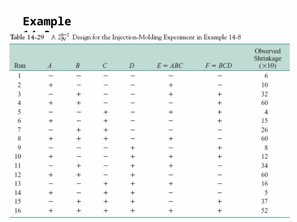
Example 14-8

14-7 Fractional Replication of the 2k Design
Example 14-8
Figure 14-33 The 24-1 design for the experiment of Example 14-8.

14-7 Fractional Replication of the 2k Design
Example 14-8

14-7 Fractional Replication of the 2k Design
Example 14-8

14-7 Fractional Replication of the 2k Design
Example 14-8

14-7 Fractional Replication of the 2k Design
Example 14-8
Figure 14-34 Normal probability plot of the effects from Minitab, Example 14-8.

14-7 Fractional Replication of the 2k Design
Projection of the 2k-1 Design
Figure 14-35 Projection of a 23-1 design into three 22 designs.

14-7 Fractional Replication of the 2k Design
Projection of the 2k-1 Design
Figure 14-36 The 22 design obtained by dropping factors B and C from the plasma etch experiment in Example 14-8.

14-7 Fractional Replication of the 2k Design
Design Resolution

14-7 Fractional Replication of the 2k Design
14-7.2 Smaller Fractions: The 2k-p Fractional Factorial

14-7 Fractional Replication of the 2k Design
Example 14-9
Example 14-8

14-7 Fractional Replication of the 2k Design
Example 14-9

14-7 Fractional Replication of the 2k Design
Example 14-9
Figure 14-37 Normal probability plot of effects for Example 14-9.

14-7 Fractional Replication of the 2k Design
Example 14-9
Figure 14-38 Plot of AB (mold temperature-screw speed) interaction for Example 14-9.


14-7 Fractional Replication of the 2k Design
Example 14-9
Figure 14-39 Normal probability plot of residuals for Example 14-9.

14-7 Fractional Replication of the 2k Design
Example 14-9
Figure 14-40 Residuals versus holding time (C) for Example 14-9.

14-7 Fractional Replication of the 2k Design
Example 14-9
Figure 14-41 Average shrinkage and range of shrinkage in factors A, B, and C for Example 14-9.

14-8 Response Surface Methods and Designs
Response surface methodology, or RSM , is a collection of mathematical and statistical techniques that are useful for modeling and analysis in applications where a response of interest is influenced by several variables and the objective is to optimize this response.

14-8 Response Surface Methods and Designs
Figure 14-42 A three-dimensional response surface showing the expected yield as a function of temperature and feed concentration.

14-8 Response Surface Methods and Designs
Figure 14-43 A contour plot of yield response surface in Figure 14-42.

14-8 Response Surface Methods and Designs
The first-order model
The second-order model

14-8 Response Surface Methods and Designs
Method of Steepest Ascent

14-8 Response Surface Methods and Designs
Method of Steepest Ascent
Figure 14-41 First-order response surface and path of steepest ascent.

14-8 Response Surface Methods and Designs
Example 14-11

14-8 Response Surface Methods and Designs
Example 14-11
Figure 14-45 Response surface plots for the first-order model in the Example 14-11.

14-8 Response Surface Methods and Designs
Example 14-11
Figure 14-46 Steepest ascent experiment for Example 14-11.


![Experimental Results on Gravity Driven Fully …narain/IJHMT_Expt_narain_G10017.pdfwaves) approach [16]. The eventual goal of this type of experiment/theory synthesis is that if one](https://static.fdocuments.us/doc/165x107/5e43b2048009457d8b0d449e/experimental-results-on-gravity-driven-fully-narainijhmtexptnarain-waves-approach.jpg)