139 D Shehova1

7/26/2019 139 D Shehova1

http://slidepdf.com/reader/full/139-d-shehova1 1/4

ANNUAL JOURNAL OF ELECTRONICS, 2014, ISSN 1314-0078

139

D. Shehova is with the Technical College by Plovdiv

University “Paisiy Hilendarski”, 4700 Smolyan, Bulgaria, e-

mail: [email protected]. Yakimov is with the Department of Electronics, Faculty of

Electronic Engineering and Technologies, Technical Universityof Sofia, 8 Kl. Ohridski Blvd, Sofia 1000, Bulgaria, e-mail:

[email protected].

Teaching PLL Fundamentals Using

MATLAB/Simulink

Daniela Antonova Shehova and Peter Ivanov Yakimov Abstract – PLL is employed in a wide array of electronic

and communications equipment and understanding its

principles is of a great importance. Simulation is an obvious

solution for teaching PLL fundamentals. MATLAB/Simulink

is a very powerful block simulation environment, most

capable for PLL. The paper discusses an approach for

teaching enabling the students to obtain sustainable

knowledge about PLL.Keywords – PLL, Simulink, MATLAB, simulation, teaching

I. I NTRODUCTION

Phase-locked loop (PLL) is a feedback loop which lockstwo waveforms with same frequency but shifted in phase[1]. The fundamental use of this loop is in comparingfrequencies of two waveforms and then adjusting the

frequency of the waveform in the loop to equal the inputwaveform frequency. Used to synchronize the phase of twosignals, the PLL is employed in a wide array of electronicand communications equipment, including microprocessorsdevices such as radios, televisions, and mobile phones. The basic blocks of the PLL are a phase detector, a low-passfilter, a variable frequency oscillator, and a divider (Fig. 1).

Fig. 1. PLL general block diagram.

Obtaining sustainable knowledge about PLL requiresunderstanding its fundamentals - loop components, loopresponse, loop stability, transient response, modulationresponse. Simulation is an obvious solution. Most oftenMATLAB will suffice for modeling and simulation. Theuse of Spice with behavioral level modeling capabilitiesmay also be useful, e.g., XSpice via SIMetrix/SIMPLIS or

PSpice. Simulink ® is a block diagram environment for

multidomain simulation and Model-Based Design [4]. It

supports simulation, automatic code generation, andcontinuous test and verification. Simulink provides a

graphical editor, customizable block libraries, and solversfor modeling and simulating dynamic systems. It is

integrated with MATLAB®, enabling incorporation

MATLAB algorithms into models and exportationsimulation results to MATLAB for further analysis.MATLAB Simulink is a very powerful block simulationenvironment, most capable for PLL. Simulink behavioralsimulation is much faster than circuit-level simulation, andas a result, there can be completed many simulations in one

day, experimenting with different implementation ideas forthe functional blocks. The behavioral simulations areinstrumental in determining the block-level specificationsthat will satisfy a given set of top-level PLL specifications.

II. BASIC BLOCKS MODEL PARAMETERS SETTING

A. Pulse Generator

The Pulse Generator block generates the referencesignal. It produces a periodic pulse train. The variablesynFr denotes the frequency of the pulse train. The period

of the pulse train is 1/synFr . To change the value of the

period, the value of the variable synFr has to be changed sothat the new value of synFr is used in all the blocks whose parameters reference the variable synFr (Fig. 2).

Fig. 2. Pulse generator model parameter setting.

B. Divide Frequency subsytems

There are two divide frequency subsystems - dividefrequency by synM and divide frequency by synN . The

7/26/2019 139 D Shehova1


ANNUAL JOURNAL OF ELECTRONICS, 2014

140

divide frequency by synM subsystem divides the frequencyof the reference signal by the variable synM . The output ofthe block is a pulse train called the frequency-dividedreference signal. This value determines the step of the

output frequency setting. The divide frequency by synN subsystem divides the frequency of the synthesized signal by the variable synN . The output of this subsystem is calledthe frequency-divided synthesized signal. At steady state itsfrequency has the same value as the output one of the synM subsystem. The value of the divisor in these subsystemscan be changed by changing the value of synM or synN (Fig. 3).

Fig. 3a. SynM value setting.

Fig. 3b. SynN value setting.

C. Phase Detector

The Logical Operator block acts as a phase detector. It

uses the XOR operation to compare the frequencies of thefrequency-divided reference signal and the frequency-divided synthesized signal. At steady state, the signal is a pulse train with frequency two times higher than the bothinputs. The reason for this is that both inputs to the block

have equal frequencies, but they are out of phase by 1/4 oftheir period. As a result, the signal after the XOR operationis a periodic pulse train with double frequency (Fig. 4).

Fig. 4. Phase detector parameters setting.

D. Analog Filter Design

The Analog Filter Design block filters high frequenciesout of the signal coming from the phase detector. The blockuses a lowpass Butterworth filter. A higher-order filter oranother filter type can be used to improve the stability of

the synthesized signal (Fig. 5). In the steady state of themodel, the amplitude of the block’s output signal is

approximately constant, with a value of 0.5. This is theaverage value of the output from the phase detector.

A Gain block multiplies the output signal from theAnalog Filter Design block by a constant to produce the

control signal.

Fig. 5. Analog filter design menu.

E. Voltage-Controlled Oscillator

The Continuous-Time VCO block generates thesynthesized signal (along with the Convert to Square Wavesubsystem) and adjusts the frequency of the synthesizedsignal according to the Voltage-Controlled Oscillator inputsignal. When the control signal is close to its steady-state,the Continuous-Time VCO block generates a signal whosefrequency is close to synFr *synN /synM . If the output

frequency drops, the control signal rises, boosting thefrequency of the output signal. If the output frequency

rises, the control signal falls, lowering the outputfrequency. The Quiescent frequency parameter is just theoscillation frequency, synFq. The difference between the block’s output signal frequency and the quiescent

frequency is proportional to the input signal, interpreted asvoltage. The quiescent frequency is set to the variablesynFq. This value can be changed in the quiescentfrequency field, or by changing the value of synFq in the

base MATLAB workspace (Fig. 6).

Fig. 6. VCO parameters setting.

III. STUDY OF FRACTIONAL-N FREQUENCY

SYNTHESIS

As an example a study of a fractional-N frequency

synthesis (Fig. 7) is chosen to explain the students theoperation of PLL and to give them skills for work withMATLAB/Simulink [2].

7/26/2019 139 D Shehova1



141

Fig. 7. Fractional-N frequency synthesis model.

The model multiplies the frequency synFr of a referencesignal by a constant synN +synM , to produce a synthesizedsignal of frequency synFr *(synN +synM ). A feedback loopmaintains the frequency of the synthesized signal at this

level. SynN is an integer and synM is a fraction between 0and 1. Two subsystems in this example are not present in

the Phase-Locked Frequency Synthesis model:Accumulator and Divide Frequency.

A. Accumulator

The Accumulator subsystem repeatedly adds the

constant synM to a cumulative sum. While the sum is lessthan 1, the output labeled "Carry" is 0. At a time step whenthe sum becomes greater than or equal to 1, the carryoutput is 1 and the cumulative sum is reset to its fractional part. The fraction of the time when the carry output is 1 isequal to synM , while the fraction of the time when it is 0 isequal to 1-synM (Fig. 8).

Fig. 8. Accumulator subsystem.

B. Divide Frequency

The Divide Frequency subsystem divides the frequency

of the synthesized signal by synN when the output of theAccumulator subsystem is 0, and divides it by synN +1

when the output is 1 (Fig. 9). As a result, the averageamount that frequency is divided by is:(1-synM )*synN + synM *(synN +1) = synN + synM (1)

Fig. 9. Divide frequency parameters setting.

The students’ task is to investigate the fractional-Nfrequency synthesis using Simulink according to thefollowing plan:

1. Setting the basic parameters:

Parameter Value

synM 0,1 ÷ 0,9

synN 10

Fr 10 MHz

Fq 101 ÷ 109 MHz2. Performing simulations for different filter type and

presenting the results for Fq [MHz] in table 1:

TABLE 1. SIMULATIONS RESULTS

synM Butterworth Chebyshev I Chebyshev II Elliptic

0,1 100,8 100,7 94,27 100,7

0,2 101,8 101,8 94,26 101,8

0,3 103,1 103 94,27 103,1

0,4 104,2 103,9 94,26 103,9

0,5 105 104,9 94,26 104,9

0,6 106 106 94,23 106

0,7 107 107,1 94,26 107,1

0,8 108 108 94,26 108

0,9 109 109,4 94,25 109,4

7/26/2019 139 D Shehova1



142

3. The presented in the table above results are visualizedgraphically using MATLAB. For this purpose the studentscreate the following source code:x=0.1:0.1:0.9;y1=[100.8 101.8 103.1 104.2 105 106 107 108 109];

y2=[100.7 101.8 103.1 103.9 104.9 106 107.1 108 109.4];y3=[94.27 94.26 94.27 94.26 94.26 94.23 94.26 94.26 94.25];y4=[100.7 101.8 103 103.9 104.9 106 107.1 108 109.4];plot(x, y1, '- g o', x, y2, '- b x', x, y3, '- r o', x, y4, '- m x',....

'MarkerFaceColor', 'k', 'MarkerSize', 5, 'LineWidth', 3)grid on, xlabel('m'), ylabel('Fq, MHz')title('Frequensy Synthesis ')legend('y1(Butterworth)','y2(ChebychevI)','y3(ChebychevII)','y4(Elliptic)')

where the arrays contain the following data: y1 - the output frequency values using Butterworthfiltration;

y2 - the output frequency values using Chebyshev Ifiltration;

y3 - the output frequency values using Chebyshev IIfiltration;

y4 - the output frequency values using Elliptic filtration.

The graphical presentation of the results is depicted onFig. 10.

0.1 0.2 0.3 0.4 0.5 0.6 0.7 0.8 0.994

96

98

100

102

104

106

108

110

m

F q ,

M H z

Frequensy Synthesis

y1(Butterworth)

y2(Chebychev I)

y3(Chebychev II)

y4(Elliptic)

Fig. 10. Output frequency plots.

Fig. 11. Pulse signals oscillograms.

The explanation of the simulation results gives thestudents knowledge about the filter usage. Chebyshev I andElliptic filtration methods have sharper slopes so the resultsare the most close to the real values. The inversed

Chebyshev approximation is not suitable for the proposedfrequency synthesis.

Fig. 12. Control signal oscillogram.

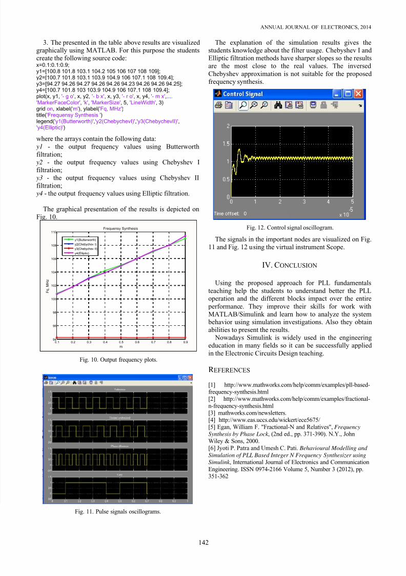
The signals in the important nodes are visualized on Fig.11 and Fig. 12 using the virtual instrument Scope.

IV. CONCLUSION

Using the proposed approach for PLL fundamentals

teaching help the students to understand better the PLLoperation and the different blocks impact over the entire

performance. They improve their skills for work withMATLAB/Simulink and learn how to analyze the system behavior using simulation investigations. Also they obtainabilities to present the results.

Nowadays Simulink is widely used in the engineeringeducation in many fields so it can be successfully applied

in the Electronic Circuits Design teaching.

R EFERENCES

[1] http://www.mathworks.com/help/comm/examples/pll-based-frequency-synthesis.html[2] http://www.mathworks.com/help/comm/examples/fractional-

n-frequency-synthesis.html[3] mathworks.com/newsletters.[4] http://www.eas.uccs.edu/wickert/ece5675/

[5] Egan, William F. "Fractional-N and Relatives", Frequency

Synthesis by Phase Lock , (2nd ed., pp. 371-390). N.Y., John

Wiley & Sons, 2000.[6] Jyoti P. Patra and Umesh C. Pati. Behavioural Modelling and

Simulation of PLL Based Integer N Frequency Synthesizer using

Simulink , International Journal of Electronics and Communication

Engineering. ISSN 0974-2166 Volume 5, Number 3 (2012), pp.351-362

139 D Shehova1

Documents

Transcript of 139 D Shehova1