1364 IEEE TRANSACTIONS ON SIGNAL PROCESSING, VOL. 55, NO. 4…tblu/monsite/pdfs/blu0701.pdf ·...

1364 IEEE TRANSACTIONS ON SIGNAL PROCESSING, VOL. 55, NO. 4, APRIL 2007

Self-Similarity: Part II—Optimal Estimation ofFractal Processes

Thierry Blu, Senior Member, IEEE, and Michael Unser, Fellow, IEEE

Abstract—In a companion paper (see Self-Similarity: PartI—Splines and Operators), we characterized the class of scale-in-variant convolution operators: the generalized fractional deriva-tives of order . We used these operators to specify regularizationfunctionals for a series of Tikhonov-like least-squares data fittingproblems and proved that the general solution is a fractional splineof twice the order. We investigated the deterministic propertiesof these smoothing splines and proposed a fast Fourier transform(FFT)-based implementation. Here, we present an alternativestochastic formulation to further justify these fractional splineestimators. As suggested by the title, the relevant processes arethose that are statistically self-similar; that is, fractional Brownianmotion (fBm) and its higher order extensions. To overcome thetechnical difficulties due to the nonstationary character of fBm,we adopt a distributional formulation due to Gel’fand. This allowsus to rigorously specify an innovation model for these fractal pro-cesses, which rests on the property that they can be whitened bysuitable fractional differentiation. Using the characteristic formof the fBm, we then derive the conditional probability densityfunction (PDF) ( ( ) ), where = ( ) + [ ]are the noisy samples of the fBm ( ) with Hurst exponent .We find that the conditional mean is a fractional spline of degree2 , which proves that this class of functions is indeed optimalfor the estimation of fractal-like processes. The result also yieldsthe optimal [minimum mean-square error (MMSE)] parametersfor the smoothing spline estimator, as well as the connection withkriging and Wiener filtering.

Index Terms—Fractional Brownian motion, fractional splines,interpolation, minimum mean-square error (MMSE) estimation,self-similar processes, smoothing splines, Wiener filtering.

I. INTRODUCTION

I N the preceding paper [1], we demonstrated the power ofthe differential formulation of splines by constructing an ex-

tended family of fractional splines. These functions are speci-fied in terms of a differential operator L, which, in the presentcase, is constrained to be scale invariant (or self-similar). Wealso investigated an alternative variational formulation which al-lowed us to recover a subset of these splines (the ones associatedwith self-adjoint operators) based on the minimization of somescale-invariant “spline energy” involving the same type of oper-ator. We used this deterministic framework to specify a generalparametric class of smoothing spline estimators for fitting dis-crete signals corrupted by noise.

Manuscript received October 12, 2005; revised June 27, 2006. The associateeditor coordinating the review of this paper and approving it for publicationwas Dr. Timothy N. Davidson. This work is funded in part by the grant 200020-101821 from the Swiss National Science Foundation.

The authors are with the Biomedical Imaging Group, Ecole PolytechniqueFédérale de Lausanne (EPFL), CH-1015 Lausanne, Switzerland (e-mail:[email protected]).

Digital Object Identifier 10.1109/TSP.2006.890845

Differential operators also naturally arise in the theory of con-tinuous-time stochastic processes; for instance, it is often pos-sible to specify a process as the solution of a stochasticdifferential equation , whose driving termis white Gaussian noise with variance —this type of repre-sentation is often referred to as the innovation model of theprocess [2], [3]. Now, in the standard case where L is shiftinvariant and its inverse is well defined in the -sense (i.e.,

), this procedure defines a stationaryprocess whose power density is . Theinterpretation is simply that L is the whitening operator of theprocess.

Interestingly, there is a perfect parallel between the determin-istic differential equations used to define general L-splines, andthe stochastic ones just mentioned above. In our previous work,we have taken advantage of this fact to derive an equivalence be-tween spline interpolation and the optimal, continuous-time es-timation of stationary processes from their integer samples [4].In particular, we showed that every continuous-time stationaryprocess with a rational power spectrum has a natural exponen-tial spline space associated with it and that this space containsthe optimal solutions of all related minimum mean-square error(MMSE) interpolation and estimation problems.

Following this line of thought, it seems quite natural toextend those stochastic results to the classical polynomialsplines [5] and their fractional extensions specified in [1]. Un-fortunately, this is far less trivial than we would have thoughtinitially because of the lack of correspondence betweenspectra and stationary processes. Indeed, the price to pay forself-similary is the zero of order in the frequency responseof L at , which makes the differential system unstableand substantially complicates the mathematical analysis. Here,as suggested by the title, the relevant stochastic processes arethose that are statistically self-similar [6]. These were charac-terized in 1968 by Mandelbrot and Van Ness [7] and namedfractional Brownian motion (fBm) because they can be viewedas an extension of Brownian motion, also known as the Wienerprocess. In this respect, we note that there is an early mentionof a link between (thin-plate) splines and fractals in a paper bySzeleski and Terzopoulos in computer graphics, the argumentbeing that both types of entities give rise qualitatively to thesame type of frequency behavior [8]. The main difficulty indealing with fBms is that they are nonstationary,1 meaning that

1It can be shown that there is no mean-square-continuous stationary processwhose covariance function is self-similar. However, a careful distributional ex-tension using Gel’fand and Vilenkin’s mathematical framework can lead to thedefinition of Gaussian stationary processes that are self-similar, discontinuous,and of infinite power (e.g., white noise) [9]. Qualitatively, these correspond tofBm’s with H < 0.

1053-587X/$25.00 © 2007 IEEE

BLU AND UNSER: SELF-SIMILARITY: PART II—OPTIMAL ESTIMATION OF FRACTAL PROCESSES 1365

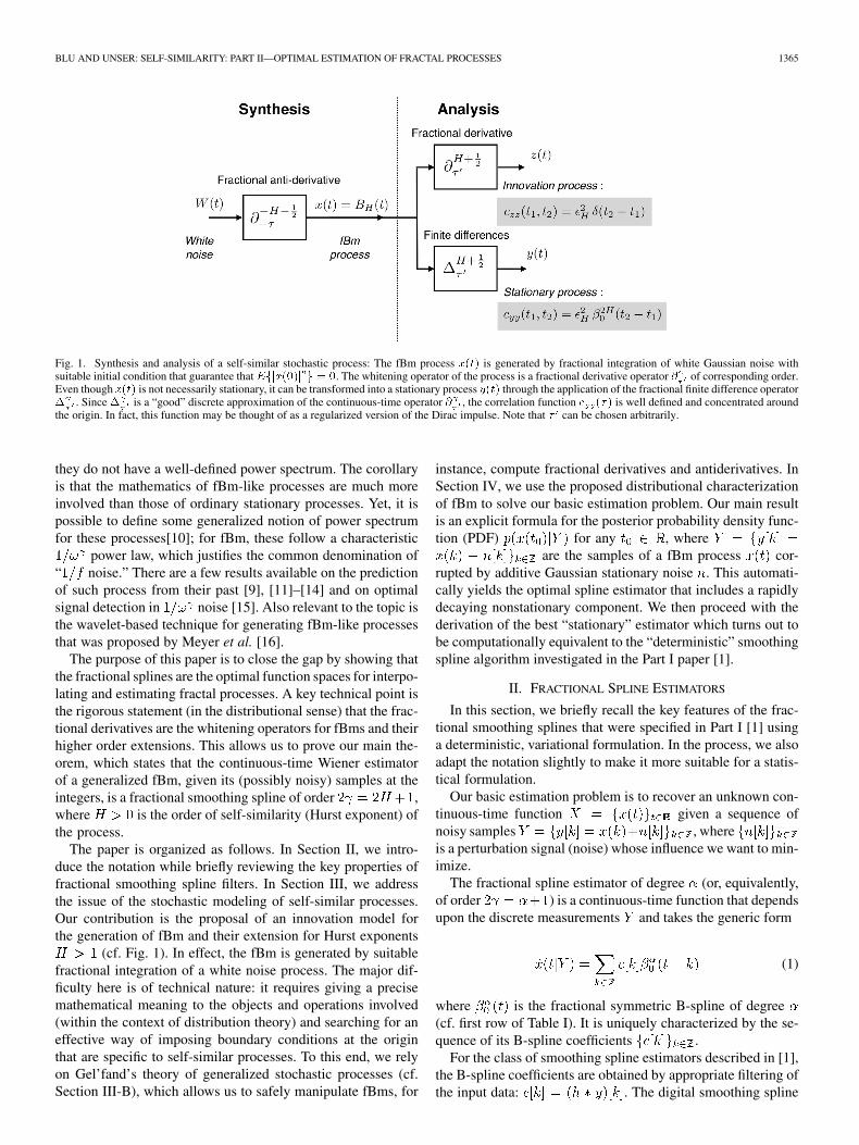
Fig. 1. Synthesis and analysis of a self-similar stochastic process: The fBm process x(t) is generated by fractional integration of white Gaussian noise withsuitable initial condition that guarantee that Efjx(0)j g = 0. The whitening operator of the process is a fractional derivative operator @ of corresponding order.Even though x(t) is not necessarily stationary, it can be transformed into a stationary process y(t) through the application of the fractional finite difference operator� . Since � is a “good” discrete approximation of the continuous-time operator @ , the correlation function c (�) is well defined and concentrated aroundthe origin. In fact, this function may be thought of as a regularized version of the Dirac impulse. Note that � can be chosen arbitrarily.

they do not have a well-defined power spectrum. The corollaryis that the mathematics of fBm-like processes are much moreinvolved than those of ordinary stationary processes. Yet, it ispossible to define some generalized notion of power spectrumfor these processes[10]; for fBm, these follow a characteristic

power law, which justifies the common denomination of“ noise.” There are a few results available on the predictionof such process from their past [9], [11]–[14] and on optimalsignal detection in noise [15]. Also relevant to the topic isthe wavelet-based technique for generating fBm-like processesthat was proposed by Meyer et al. [16].

The purpose of this paper is to close the gap by showing thatthe fractional splines are the optimal function spaces for interpo-lating and estimating fractal processes. A key technical point isthe rigorous statement (in the distributional sense) that the frac-tional derivatives are the whitening operators for fBms and theirhigher order extensions. This allows us to prove our main the-orem, which states that the continuous-time Wiener estimatorof a generalized fBm, given its (possibly noisy) samples at theintegers, is a fractional smoothing spline of order ,where is the order of self-similarity (Hurst exponent) ofthe process.

The paper is organized as follows. In Section II, we intro-duce the notation while briefly reviewing the key properties offractional smoothing spline filters. In Section III, we addressthe issue of the stochastic modeling of self-similar processes.Our contribution is the proposal of an innovation model forthe generation of fBm and their extension for Hurst exponents

(cf. Fig. 1). In effect, the fBm is generated by suitablefractional integration of a white noise process. The major dif-ficulty here is of technical nature: it requires giving a precisemathematical meaning to the objects and operations involved(within the context of distribution theory) and searching for aneffective way of imposing boundary conditions at the originthat are specific to self-similar processes. To this end, we relyon Gel’fand’s theory of generalized stochastic processes (cf.Section III-B), which allows us to safely manipulate fBms, for

instance, compute fractional derivatives and antiderivatives. InSection IV, we use the proposed distributional characterizationof fBm to solve our basic estimation problem. Our main resultis an explicit formula for the posterior probability density func-tion (PDF) for any , where

are the samples of a fBm process cor-rupted by additive Gaussian stationary noise . This automati-cally yields the optimal spline estimator that includes a rapidlydecaying nonstationary component. We then proceed with thederivation of the best “stationary” estimator which turns out tobe computationally equivalent to the “deterministic” smoothingspline algorithm investigated in the Part I paper [1].

II. FRACTIONAL SPLINE ESTIMATORS

In this section, we briefly recall the key features of the frac-tional smoothing splines that were specified in Part I [1] usinga deterministic, variational formulation. In the process, we alsoadapt the notation slightly to make it more suitable for a statis-tical formulation.

Our basic estimation problem is to recover an unknown con-tinuous-time function given a sequence ofnoisy samples , whereis a perturbation signal (noise) whose influence we want to min-imize.

The fractional spline estimator of degree (or, equivalently,of order ) is a continuous-time function that dependsupon the discrete measurements and takes the generic form

(1)

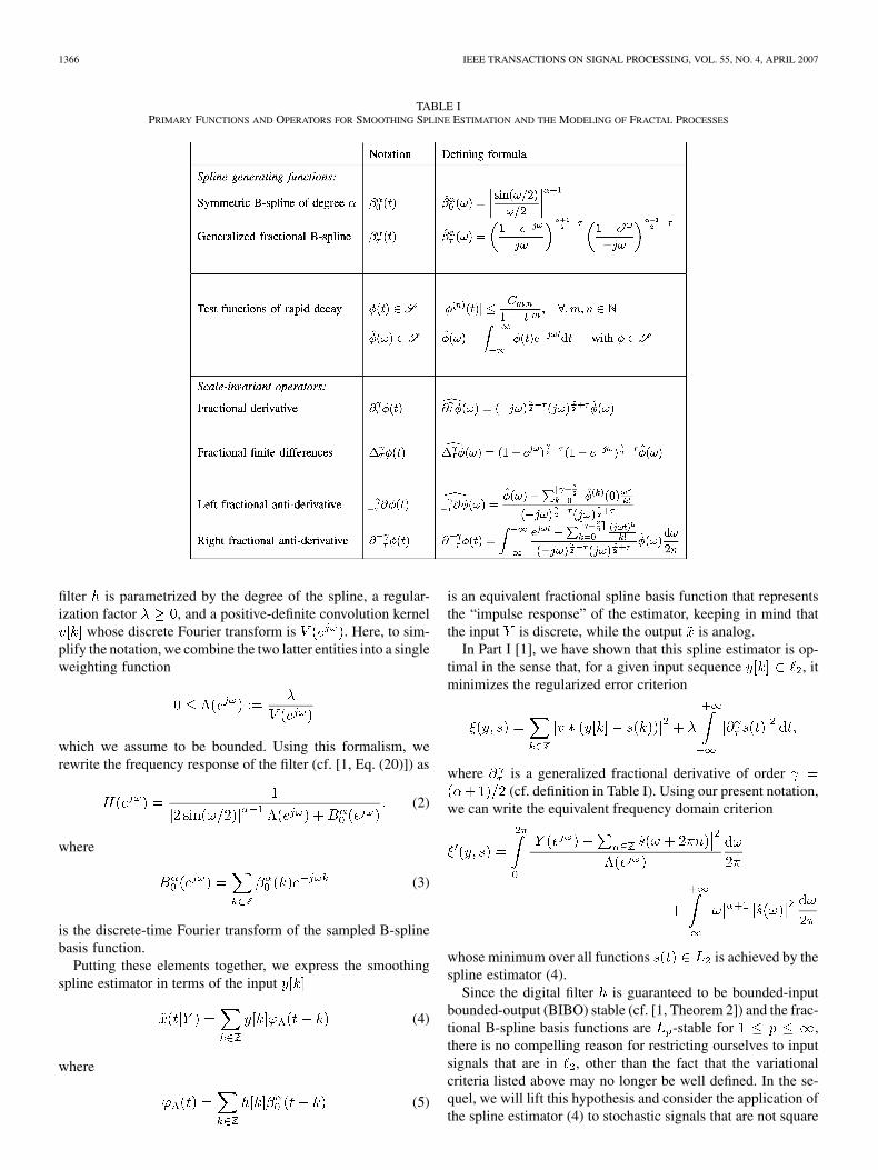
where is the fractional symmetric B-spline of degree(cf. first row of Table I). It is uniquely characterized by the se-quence of its B-spline coefficients .

For the class of smoothing spline estimators described in [1],the B-spline coefficients are obtained by appropriate filtering ofthe input data: . The digital smoothing spline


TABLE IPRIMARY FUNCTIONS AND OPERATORS FOR SMOOTHING SPLINE ESTIMATION AND THE MODELING OF FRACTAL PROCESSES

filter is parametrized by the degree of the spline, a regular-ization factor , and a positive-definite convolution kernel

whose discrete Fourier transform is . Here, to sim-plify the notation, we combine the two latter entities into a singleweighting function

which we assume to be bounded. Using this formalism, werewrite the frequency response of the filter (cf. [1, Eq. (20)]) as

(2)

where

(3)

is the discrete-time Fourier transform of the sampled B-splinebasis function.

Putting these elements together, we express the smoothingspline estimator in terms of the input

(4)

where

(5)

is an equivalent fractional spline basis function that representsthe “impulse response” of the estimator, keeping in mind thatthe input is discrete, while the output is analog.

In Part I [1], we have shown that this spline estimator is op-timal in the sense that, for a given input sequence , itminimizes the regularized error criterion

where is a generalized fractional derivative of order(cf. definition in Table I). Using our present notation,

we can write the equivalent frequency domain criterion

whose minimum over all functions is achieved by thespline estimator (4).

Since the digital filter is guaranteed to be bounded-inputbounded-output (BIBO) stable (cf. [1, Theorem 2]) and the frac-tional B-spline basis functions are -stable for ,there is no compelling reason for restricting ourselves to inputsignals that are in , other than the fact that the variationalcriteria listed above may no longer be well defined. In the se-quel, we will lift this hypothesis and consider the application ofthe spline estimator (4) to stochastic signals that are not square


summable. It is important to note that this does not change any-thing from a computational point of view, meaning that the fastsmoothing spline algorithm introduced in [1, Sec. IV] and thecorresponding frequency domain analysis remain valid.

III. STOCHASTIC MODELING OF SELF-SIMILAR PROCESSES

To justify the use of the above smoothing spline estimatoron statistical grounds, we first need to introduce an appro-priate mathematical framework that allows us to characterizefractal-like processes and to apply linear operators to them,including the fractional derivatives listed in Table I. Since thiscannot be handled by standard stochastic calculus, we hadto turn to Gel’fand and Vilenkin’s theory of generalized sto-chastic processes which constitutes the statistical counterpartof Schwartz’s theory of distributions.

A. Self-Similar Processes: Review of Standard Results

There are a number of technical difficulties with the modelingof self-similar processes, with fBm being the most prominentexample. This is primarily due to the fact that these processes arenonstationary, meaning that their spectral power density cannotbe defined in the conventional sense. Fortunately, the -lag in-crement derived process , wheredenotes the realization of an fBm-like process, is zero-mean,second-order stationary.

In the statistical literature, a process whose increments arestationary is referred to as being intrinsic stationary. These pro-cesses are often characterized by their variogram [17]

which measures the variance of the increment process asa function of the time lag.

A real valued stochastic process is self-sim-ilar with index (or Hurst exponent) if, for any

where denotes the equality of all underlying finite-dimen-sional distributions.

The fBm with Hurst exponent is a zero-meanGaussian process that is both self-similar and intrinsically sta-tionary [7]. In particular, this implies that its variogram is self-similar of order (in the sense that ) andis therefore given by

(6)

where is simply a scaling factor (cf. [1, proof of Propo-sition 1]). The variance of the fBm has the same self-similarfunctional form

(7)

which is time dependent, confirming that the process isnonstationary.

If we know both the time-varying variance and the variogramof the process, we easily obtain the autocorrelation function, dueto the relation

In the case of the fBm process, this yields the following explicitform of the autocorrelation:

(8)

which is also self-similar of order . Conversely, it can beshown that the 2-D function defined by (8) is nonnegative defi-nite (see Theorem 1 below) and that it is the only possible para-metric form of correlation that corresponds to a process that isboth self-similar and intrinsically stationary [18].

The notion of intrinsic stationarity can be further generalizedby considering processes whose th-order increments are sta-tionary [12], [19]. Among those, one can also identify the onesthat are self-similar, which leads to an extended notion of frac-tional Brownian motion for larger Hurst exponents such that

, where is the order of the increment. Suchprocesses can be obtained, for example, from the -fold integra-tion of a conventional fBm with suitable initial conditions [20].This leads to an autocorrelation function of the form

(9)

where is a constant and . In the litera-ture, the constant is sometimes expressed as

, where is a spectral energy factor;the standard normalized case corresponds to the choiceand .

B. Generalized Stochastic Processes: Gel’fand–Vilenkin’sApproach [21]

In order to perform linear operations such as differentiationon random processes, a fruitful approach is to consider themas random distributions and to extend the applicability of thedistributional calculus to these processes. In particular, this for-malism provides a rigorous definition of white noise, whichplays such as fundamental role in statistical signal processing.A very stimulating and fundamental presentation of this theorycan be found in [21].

Although Gel’fand and Vilenkin’s approach is a naturalextension of the now classical theory of distributions [22],it seems to have been somewhat neglected in the standardliterature on random processes, including fBm’s. One notableexception relating to signal processing is [23]. By contrast,the Itô stochastic calculus and its Stratonovich variant havereceived a much greater attention, in particular, in statisticalphysics and financial mathematics [24], [25]. Both types of


approaches have their advantages and limitations; for instance,the Itô calculus can handle certain nonlinear operations onrandom processes that cannot be dealt with the distributionalapproach. Gel’fand’s theory, on the other hand, is ideally suitedfor performing any kind of linear operations, including some,such as fractional derivatives, which are extremely cumbersometo define in a traditional (nondistributional) framework.

Most readers may recall that a distribution is not definedthrough its point values (samples), but rather through a seriesof scalar products (linear functionals) with all test func-tions (Schwartz’s class). These test functions are indef-initely differentiable and they, as well as all their derivatives,have very rapid decay (i.e., faster than ).In an analogous fashion, a generalized stochastic processis not defined by the probability law of its pointwise samples

, but by the probability lawof its scalar products with arbitrary test functions .

Specifically, given , is a random variablecharacterized by a probability density . The character-istic function of this random variable is used to define a func-tional of , as follows:

where is the expectation operator. This functional iscalled the characteristic form of the process . It is important tounderstand that it concentrates all the information available onthe generalized stochatic process . For instance, if one wantsto access the joint probability of the random variables

, then it suffices to takethe inverse Fourier transform ofwith respect to . This is because the prob-ability density of the set of random variables isgiven by

Conversely, if is a continuous form of positive type2 andsatisfies , then it is the characteristic form of a gener-alized stochastic process . The continuity of the functionalexpresses the fact that tends to when tends to

as ; it is an essential ingredient that allows the exten-sion of the characteristic form to potentially larger functionspaces than . For instance, if is continuous with respect tothe -norm then, due to the density of in , we may extendthe functional to arbitrary functions of . For continuousprocesses such as fBm, we can even let tend to , the Diracdistribution: the continuity property of the characteristic formwill ensure that is well defined.

Conceptually, this means that the characteristic form can beviewed as the distributional, infinite-dimensional extension ofthe classical characteristic function. To get a better feeling for

2i.e., if the matrix Z = [Z(� � � )] is positive irrespective ofN 2 n f0g and of the choice of � 2 S .

this connection, we note that the characteristic function (i.e., theFourier transform of the probability density) of the sampleof a stochastic process is defined by , which canalso be expressed as ; this corresponds to a one-dimen-sional analysis of the process with the test functions

parametrized by . The argument obviously alsoholds in higher dimensions by considering the -dimensionalsubspace of test functions with

.The advantage of working with scalar products instead of

point values is that it is possible to exploit duality propertiesto perform linear operations such as differentiation, Fouriertransforms or convolutions. For instance, using the definitions

, we are able to compute the fractionalderivative of a stochastic process. This can be moved automati-cally to the characteristic form

(10)

More generally, if is some filter, the characteristic form ofis given by , where .

Similarly, using the definition , the charac-teristic form of the Fourier transform of a stochastic process isgiven by

(11)

The case of generalized, zero-mean Gaussian processes is espe-cially simple to deal with since they are completely defined bytheir mean and autocorrelation. Specifically, if is thecorrelation form3 of the zero-mean process , then its charac-teristic form is given by

(12)

Conversely, if is a continuous positive distribution of ,then (12) defines a generalized zero-mean Gaussian process.Stationary processes have a simpler characteristic form

(13)

where is a filter such that is the power spectraldensity of the process . Of particular interest is the case ofthe normalized Gaussian white noise , which is defined viaits characteristic form

Applying Parseval identity and the definition (11) of the Fouriertransform of a stochastic process, we easily get the “intuitive”result that the Fourier transform of a white noise is a white noiseas well.

However, if we lift the Gaussian hypothesis, other versions ofwhite noise processes can be obtained, such as the generalizedPoisson process, which has the following characteristic form:

3defined by hc (t; t ); �(t) (t )i = Efhx; �ihx; ig for all �; 2 S .


In their book, Gel’fand and Vilenkin give the explicit expres-sion of the characteristic form of an even broader class of non-Gaussian white noiselike processes [21].

C. Fractional Integrals/Antiderivatives

One of the classical definition of fBm involves a fractional in-tegral of a Wiener (or Brownian motion) process [7], [18]. It istherefore tempting to introduce an extended family of integraloperators (fractional antiderivatives) that are inverse operatorsfor , where . To this end, we have to make the distinc-tion between left and right inverse denoted, respectively, byand . When , we propose the following operators:

and

(14)

When is regular and decreases fast enough,4 defines atrue function, which is either in when is not a half-integer,or is continuous and slowly decreasing (but not in ) when isa half-integer. It is easy to verify that satisfiesfor every function of , i.e., Identity.

Moreover, it can be checked that and are adjoint ofone another (in a similar way as and are adjoint), i.e.,

when and are in . Due to duality,we can thus claim that , i.e.,Identity.

This allows to extend the right fractional derivative inverseto a subset of tempered distributions according to the

rule

It is interesting to note that both types of antiderivative op-erators are scale invariant of order . Intuitively, they maybe thought of as (fractional) integrals to which one has im-posed special boundary conditions at the origin. This has alsothe benefit of producing a result that is reasonably localized,i.e., square ntegrable in the case when . The left an-tiderivative operator, for instance, has a special Dirac distribu-tion annihilation property in the sense that , for

, where . The right antiderivativeoperator, on the other hand, will produce a function (or distri-bution) that has a th-order zero at theorigin: , for . When we are dealingwith a function, this can be achieved by correcting the usual in-tegral with a suitable polynomial that is in the null space of .In both cases, these are properties that are strictly tied to theorigin , indicating that the operators are not shift invariant.

Due to the above distributional relations, we can readilyapply these antiderivative operators to a wide class of gen-eralized stochastic processes , in particular, the Gaussianstationary ones specified by (26). For instance, by using the

4For instance, when is not a half-integer, we may wish to ensure thatthe remainder of the Taylor development of �̂(!) near ! = 0 be at leastO(j!j ) for some positive ", and that j�̂(!)jd! < 1, which isautomatically satisfied when � 2 S .

definition , we can directly move theright antiderivative to the characteristic form, which yields

(15)

Of course, the restriction here is that the right-hand side of(15) be well defined, which will typically be the case when

.

D. Distributional Characterization of fBm

We now present our first theoretical result on the characteri-zation of fBm.

Theorem 1: The usual fractional Brownianmotion process is characterized by the form

(16)

where , with the constantbeing defined according to (6) or (8).

Proof: We already know that an fBm is a Gaussian processwith correlation .We thus only have to prove that

In order to do this, we choose and introduce the functionwhose Fourier transform is

. Obviously,tends to when . More

precisely, Lebesgue dominated5 convergence theorem ensuresthat tends towhen .

Then, we observe that

because of the following Fourier equivalences:•

;• ;• .Let us denote by the integrable function

. We have the limitresult . Moreover,

is dominated, up to a constant, by. Finally, using Lebesgue dominated convergence the-

orem, we obtain the claimed Fourier expression

5Notice that jc (t; t )�(t)�(t )j is “dominated” by (jtj + jt j + jt �t j )j�(t)�(t )j, which is integrable.


Note that this proof is also a direct method for showing thatthe expression (8) effectively defines a correlation (i.e., a posi-tive quadratic form).

It is also possible to extend the expression (16) by making useof the left fractional antiderivative of ,defined in Section III-C. Note that is an arbitrary-freeparameter. Thanks to this notation, we rewrite the characteristicform of the fBm as

(17)

The advantage of this formula is that it also yields a natural ex-tension of the fBm for noninteger Hurst exponents . Notethat positive integer values of are excluded because they cor-respond to antiderivatives that are not necessarilysquare integrable. Using the same technique as in Theorem 1,it is then possible to compute the autocorrelation of the processdefined by (17), resulting in a form that is identical to (9). Thisalso yields a direct relation between the amplitude factor in(17) and the constant in (9), as follows:

(18)

This shows that the generalized fBm that is concisely defined by(17) with is in fact equivalent to the one introducedby Perrin et al. with the help of more traditional techniques [20].

By setting in the definition (17), we see that, for, we have . This results in

, i.e., the usual derivative of an extended fBm of ex-ponent is an extended fBm of exponent . More gen-erally, we can show that an extended fBm with nonintegerHurst exponent is -times continuously differentiable andthat is a usual fractional Brownian motionwith Hurst exponent . In fact, by substituting

in (17), we observe that the Fourier transform of theprobability density of equals 1, which meansthat with probability one. Likewise, we can showthat an extended fBm with exponent is -times continu-ously differentiable and that all its derivatives vanish at :

for .

E. Whitening Properties of the Fractional Derivatives

We now wish to reinterpret the formula (17) that definesboth the usual fBm and the “extended”one . By using the characteristic form

of the normalized Gaussianwhite noise and the duality between right and left primitive(10), we identify the characteristic form of the fBm with thecharacteristic form of , as follows:

which proves the identity between the two processes.

Proposition 1: The extended fractional Brownian motionwith arbitrary noninteger positive Hurst exponent can beexpressed as a right th antiderivative of a Gaussianwhite noise

(19)

As a corollary, we get that the th derivative of anfBm is a white noise

(20)

which follows from the right-inverse propertyIdentity.

Note that, for , the formula (20) is equivalentto the one that was proposed in [20, eq. (6)].

F. Fractional Increment Process

As mentioned in Section III-A, the standard approach fordealing with intrinsically stationary processes is to considertheir increment so that the problem reduces to the characteriza-tion of a stationary process. Alternatively, when the process isintrinsically stationary of order , one can apply an th-orderdifferentiator, which yields a (generalized) derived process thatis stationary as well [12], [19].

Here, we propose another possibility that is specifically tai-lored to the characterization of th-order self-similar processes.It is stochastic transposition of the localization techniquediscussed in [1, Sec. II and III]. Specifically, we chose toapply a discrete operator—the th-order fractional finite dif-ference—that closely approximates the whitening operator ofthe process (i.e., ). This produces a derived process that isstationary, essentially decorrelated, and yet well defined in theclassical sense (i.e., mean-square continuous) for .

Proposition 2: Let be an fBm with nonin-teger Hurst exponent . Then, the derived process

is zero mean, stationary with covariancefunction

i.e., can be expressed as the convolution of a normalizedGaussian white noise with a fractional B-spline according to

Proof: Using the definition of (cf. Table I) and the factthat its adjoint is simply , we have that

. Moreover, expressing as an antiderivativeof white noise according to (20) and using the duality definitionfor , we find that

It is now a simple matter to verify by applying the definition (14)that . The result then follows by noticingthat .

Practically, this means that we have at our disposal a digitalfilter that we can apply to —or to its sampled values


—to produce an output signal (respectively, output se-quence) that is stationary, with a very short correlation distanceand therefore much easier to handle mathematically. The wholeconcept is schematically represented in Fig. 1.

IV. OPTIMAL ESTIMATION OF FRACTAL-LIKE SIGNALS

We are now ready to investigate the problem of the MMSE es-timation of fBm signals. To this end, we will first derive the pos-terior distribution of at a fixed location given a seriesof noisy samples of a fBm with Hurst exponent . Inparticular, we will establish that the posterior mean is a fractionalspline of degree , which justifies the use of spline estimators.The next step will be to specify a Wiener-like filtering algorithmthat will perform the MMSE estimation of simultaneouslyfor all . We will show that this can be achieved via an ap-propriate tuning of the smoothing spline algorithm described inSection II and that the solution is also applicable for general-ized fBm’s with Hurst exponents greater than 1.

A. Posterior Estimation of fBm

Let be an fBm with Hurst exponent . We supposethat we are observing the signal indirectly through a series ofnoisy measurements at the integers , where

is additive stationary noise that is independent from .The noise is zero mean and is characterized by its second-orderstatistics . Our goal is to constructthe best estimator of given the measurements . To get acomplete handle on this problem, we derive the posterior distri-bution , which fully specifies the information aboutthe signal that is contained in the measurements.

Theorem 2: Let be a realization of an fBmof noninteger Hurst exponent . Then, the pos-terior probability density of given the measurements

, where is a zero-meanGaussian stationary noise independent of with autocorre-lation , is the Gaussian density

with time-varying mean

(21)

where is the fractionalsmoothing spline of degree specified by (4), (5), and(2) in Section II with

(22)

The conditional variance is given by

(23)

with

(24)

where is the equivalent smoothing spline basis functiondefined by (5).

Our proof of this result, which uses the characteristic form ofthe fBm, is given in Appendix I.

As a direct application of Theorem 2, we get the MMSE esti-mator of the fBm process , which is simply the conditionalmean [3]. The key point for our purpose is that thisestimator is a fractional spline, albeit not exactly the smoothingspline solution (4) that we may have wished for initially.

Corollary 1: Consider the noisy samples of an fBm process, as specified in Theorem 2. Then, the MMSE esti-

mator of given is the function defined in Theorem2, which is a fractional spline of degree . The correspondingminimum estimation error at location is

as specified in (23).The above results call for the following comments.

1) The optimal fBm estimator is the sum of two termsthat are both fractional splines of degree . The firstcomponent is precisely the smoothing spline fitof , as specified in Section II, with the optimal choice of

given by (22). The second term isa nonstationary correction that ensures that the estimate iszero at , which is consistent with the property that

is zero with probability one.2) The variance of the estimator is made up of two terms as

well. The first is 1-periodic. The second is a correc-tion that expresses the fact that the optimal spline estimateis more accurate near the origin because of the preferencethat is given to the value zero.

3) Interestingly, the correction function is the fractionalsmoothing spline fit of the autocorrelation of the noisewhose value at the origin has been normalized to one. Since

and takes its maximum for , one canexpect this function to decay rapidly as one moves awayfrom . For instance, when the noise is white, then

, which typically decreases like; that is, the rate of decay of the fractional

B-splines (cf. [26, Theorem 3.1]).4) When the measurement noise is zero, we have that

and . Then,corresponds to the fractional spline

interpolation of the input signal . This is equivalent to asmoothing spline estimate with . As expected, theestimation error is zero at the integers because ofthe interpolation property of the underlying basis function

.5) The optimal estimator is undistinguishable from

the smoothing spline solution in the following sit-uations: a) when the measurement noise is negligible, b)when , which may happen because of a) orsimply by chance, and c) in all cases for sufficientlylarge, that is, as one moves away from the origin, whichhas a very special status due to the self-similarity of theunderlying process.

6) An efficient way to implement the estimator is to applythe Fourier domain algorithm that was presented in [1].The procedure is to first run the algorithm on toobtain the smoothing spline . Second, one applies


the same algorithm to the autocorrelation sequence of thenoise . One then corrects by subtracting areweighted version of the latter spline so as to produce aresult that is zero at the origin.

7) The Hurst exponent of the standard Wiener (or Brownianmotion) process is . This corresponds to a simplepiecewise linear spline estimator with . In the noise-free case, we recover a classical result by Lévy [11] thatstates that the optimal estimator of a Brownian motionprocess is obtained by linearly interpolating the samples.In that case, the estimate is entirely determined by the twoneighboring samples. This is not so for other values of(or when ) because the smoothing spline filtergenerally has an infinite-impulse response, which inducescoupling.

If one excludes the simpler case of Brownian motion, thepresent results on the prediction of fractal processes are new tothe best of our knowledge. In principle, they should also be gen-eralizable for fBm’s with , but we expect the formulasto become more complicated. In the sequel, we will investigatethe general case as well but adopt a less frontal approach bysearching for the optimal estimator within the slightly more re-strictive class of Wiener-filter-like (or stationary) solutions.

B. Wiener Filtering of Fractal Processes

The main point that differentiates the optimal fBm estimatorgiven by (21) from that of a stationary process (cf. [4, Theorem5]) is the correction term , which makes the esti-mator vanish at the origin. Its presence is a consequence of thefBm being nonstationary. This lack of stationarity is obviously asource of complication; it requires the use of an advanced math-ematical formulation and makes the task of finding the best es-timator much more difficult.

While we have at our disposal a general closed-form solu-tion for , it may be justifiable in practice to discard thesecond, nonstationary part of the MMSE estimator for the fol-lowing reasons.

1) The exact location of the origin ( in our model) willrarely be known (or controllable) in practice, especially, ifwe are dealing with time series.

2) The Wiener-like estimators that are available for stationaryprocesses have the advantage of computational simplicity.The same can be said for the smoothing spline part of

, which can be implemented by digital filtering ofthe input data.

3) The estimation error in Corollary 1 does not behave likethe estimation error of a stationary process, which is nec-essarily periodic (cf. Appendix II). Instead, one may wishthe wholeness of the nonstationary behavior of the fBm tobe captured by the linear estimator, whilst the estimationerror would be indistinguishable from the estimation errorof a stationary process.

4) There is an alternative “kriging” formulation from the fieldof geostatistics that yields the best linear unbiased (BLU)estimator of from sampled data (typically, nonuni-form and multidimensional) [17], [27]. This nonparametricestimator is computed from the variogram (which does notinclude absolute positional information). Under suitable

conditions, this estimator is also known to be the solutionof a variational spline problem [28], [29].

Because of these considerations, it makes good sense to searchfor a suboptimal solution that has the simplicity of a stationary(or Wiener) estimator. In particular, we want to find out whetheror not we can improve upon the smoothing spline estimator

. The key requirement for such a formulation is expressedby Remark 3), which implies a restriction on the possible linearestimators, as described by the following proposition.

Proposition 3: Let be an fBm of arbitrary (noninteger)Hurst order and its noisy samples, where

is a zero-mean Gaussian stationary discrete process that isindependent of . We build the linear estimator of :

(25)

In order for the estimation error to behavelike the estimation error of a stationary process, it is necessaryand sufficient that

for (26)

in the sense of distributions.The proof is given in Appendix II.The interesting aspect of this result is that it allows us to

evacuate the difficulties associated with the nonstationary char-acter of fractal processes. It is also suggests that the root of theproblem lies within the (random) polynomial part of the signal,which is included in the null space of the whitening operator

. In fact, the presence of this null-space component issomewhat artificial for it is only here to ensure that the fBmhas the correct boundary conditions at the origin. Thus, a pos-sible interpretation of Proposition 3 is that the fBm can be madestationary through the removal of its polynomial trend, whichis entirely captured by any estimator satisfying (26). Inciden-tally, this polynomial reproduction property also plays a funda-mental role in wavelet theory [30], [31]. Specifically, when weperform a wavelet analysis of order of an fBm, thepolynomial component of the process is entirely projected ontothe coarser scale approximation with the consequence that thediscrete wavelet coefficients end up being stationary within anygiven scale. This is the fundamental reason why wavelets actas approximate whitening operators for fractal-like processes[32], [33].

For , we also note that the “stationarizing” hypothesisis in fact equivalent to the no-bias constraint that is used forderiving unbiased kriging estimators [17], [27]. In that particularframework, the random process to estimate is expressed as thesum of an unknown constant (the trend) and a random processof known variogram.

Under the “stationarizing” hypothesis (26), we are able toprovide the best linear estimator of a fBm. Not so surprisingly,when , this estimator is precisely the first term of(21) that was given in Theorem 2, namely . Note that theresult below is valid for values of larger than 1 as well.

Theorem 3: Let be an fBm of arbitrary (noninteger)Hurst order and its noisy samples, where


is a zero-mean Gaussian stationary discrete process withautocorrelation , independent of . Then, theleast mean-square linear estimator (25) satisfying the “station-arizing” conditions (26) is given by

where, as in Theorem 2, is the smoothing spline of degreedefined by (5) and (2), with chosen according to (22). The

variance of the estimation error is given by

For a proof, see Appendix III.This result closes the loop by showing that the optimal esti-

mator of an fBm is indeed a smoothing spline with matching pa-rameters. In particular, the spectral regularization shouldbe set proportional to the power spectrum of the noise.

For instance, when the measurement noise is white with vari-ance , then is a scalar that is inverselyproportional to the signal-to-noise ratio. This means that thesmoothing effect of the spline gets stronger as the power of thenoise increases, which is consistent with our expectation. Underthose circumstances, the effect of the smoothing spline is analo-gous to that of a Butterworth filter of order with a cutofffrequency .

Theorem 3 also gives an explicit expression for the estima-tion error. By considering the expression for given by (18),we observe that coincides with the primaryvariance component in Theorem 2 when .Note that this error is a symmetric 1-periodic function that isminimal at the integers. We expect it to take its maximum atthe half-integers because these points are the furthest away fromthe sampling locations (integers). We also expect the variance toincrease and to flatten out as the smoothing gets stronger, thatis, when is large relative to . In that respect, thesecond variance term in (23), , quantifies the loss ofperformance of the stationary estimator in Theorem 3 over theoptimal one specified in Corollary 1. Here, too, in concordancewith what has been said earlier in Section IV-A, this variancebias can be expected to decrease rapidly as one moves awayfrom the origin. This provides some solid, quantitative justifi-cation for using the stationary solution (smoothing spline) as asubstitute for the optimal one.

Among the proposed solutions, one can single out thesmoothing splines of odd degrees , which cor-respond to the optimal solution for the estimation Brownianmotion ( (linear splines) for ) and its generalizedcounterparts (in particular, (cubic splines) for ).It is noteworthy that the basic versions of these estimators havea fast recursive implementation [34]. One surprising findingof our investigation is that there is no fractal interpretation forthe fractional smoothing splines of even degree (i.e., ),whose building blocks are not piecewise polynomials, butrather “radial basis functions” of the type [26].Thus, an open question is whether or not there exist a class

of (non-self-similar) processes corresponding to these basisfunctions, or equivalently, a positive-definite form(similar to (9)) that is made up of such building blocks.

Finally, we note that the smoothing spline solution in The-orem 3 for is equivalent to the BLU estimator thatcould have been derived using the kriging formalism with com-patible hypotheses (cf. [35] for a treatment of the multidimen-sional case). The key point, however, is that the present cardinalspline framework also yields a fast algorithm that is generallynot available for kriging. Since kriging is originally designedfor dealing with nonuniform data, the standard approach is torestrict the data to a given number of neighbors of (whichis suboptimal) and to recompute the estimator by solving thenormal equations for each position . Clearly, the advantage ofusing splines is that the optimal solution can be com-puted at once for using all available data. This is com-putationally much more efficient, but only possible because weare taking advantage of the shift-invariant structure provided bythe uniform grid.

V. CONCLUSION

In this pair of papers, we have established a formal connectionbetween deterministic splines and stochastic fractal processes(fBm’s). The fundamental, unifying relation that appears in bothcontexts is the differential equation

(27)

that defines a self-similar system with continuous-time inputand output . This characterization is complete in the

sense that the fractional derivative , which is indexed by theorder and an asymmetry parameter , spans the whole classof differential operators that are both shift and scale invariant.

We can formally construct all the varieties of deterministicfractional splines identified in [1] by exciting the system with aweighted stream of Dirac impulses ,where the ’s are some suitable coefficients. Likewise, wehave shown that we could generate all brands of fBm’s, in-cluding the generalized ones with Hurst exponent

, by driving the system with white Gaussian noise.While the above differential description is appealing concep-

tually, we must be aware that it is fraught with technical dif-ficulties. Indeed, the price to pay for self-similarity is that thesystem (27) is unstable with a pole of order at . Inparticular, this means that the Green function of —the fun-damental building block of the fractional splines—is not in .Likewise, the generalized stochastic processes that are gener-ated by (27) are nonstationary. This calls for a special mathe-matical (distributional) treatment and also requires the specifi-cation of boundary conditions. Another nontrivial aspect is thatthe fractional operators are typically nonlocal, in contrast withthe classical integer-order derivatives.

The connection also extends nicely beyond the generationprocess. For instance, we have shown that the MMSE estimator

of an fBm with Hurst exponent given its—possibly,noisy—samples at the integers lies in a fractional spline space ofdegree . We derived the corresponding smoothing spline es-timator that can be assimilated to a hybrid version of the Wiener


filter for which the input is discrete and the output analog. In par-ticular, we are able to specify the Wiener filter for the Wienerprocess (with ) bringing together two seemingly in-compatible aspects of the research of Norbert Wiener. In thatparticular case, the optimal estimator happens to be a piece-wise-linear smoothing spline estimator that has a fast recursiveimplementation. As for the estimators for arbitrary values of ,we have shown that they could all be implemented efficiently bymeans of an FFT-based algorithm.

APPENDIX IPROOF OF THEOREM 2

We will proceed in three main steps: first, we derive thegeneral expression of the (Gaussian) posterior distributionof given a finite number of measurements of ;second, we calculate the expression of the posterior expectationof given for ; finally, we evaluate theexpression of the posterior standard deviation of given

.a) Step 1—Posterior probability of : Taking a more

general point of view, we first compute the posterior densityprobability of given measurements , where

. We will then setand to get the desired result.

Using Bayes’ rule, we have

We thus have to compute the joint probability density of. This will be done

through its Fourier transform; i.e., its characteristic function,which is expressed using and , the characteristic formsof the processes and

where we have denoted

Performing the inverse Fourier transform of this expression, weobtain the posterior probability density of given

This is a Gaussian density with mean and variance, where . Using the

definition of , , and , and denoting by its th component,has to satisfy

(28)

for all .b) Step 2—Computation of : We let tend to

infinity and observe that finding from the set of (28) is stillwell posed because the quadratic form characterized by the(infinite) matrix is positive definite; i.e., if there isa solution—which is not ensured when —then thissolution is unique.

We will reinterpret (28) from an interpolation view-point. By inspection of (8), we observe that

is in thespan . Denoting by , theunique interpolating function that belongs to this span,6 we thushave the interpolation formula

where is the function of specified in (24); the secondline above has been obtained by using the interpolation condi-tion and the fact that . This iden-tity can also be reformulated using a smoothing spline basis

: , where

6In Fourier variables, ' is obtained by '̂ (!) = �̂ (!)=B (e ).


To do this, we write

(29)

which allows to express in termsas

Replacing in the interpolation formula, we get

The second term on the right-hand side is evaluated as

This shows that as posed by (29) satisfies, which is precisely

(28) up to a factor 1/2. is thus the solution we arelooking for, which implies that

The last technical step is to show that the random quan-tity is well defined (convergent) almost surely; thisis ensured by the fact that decreases fast enough

to tame the divergence of as.

c) Step 3—Computation of : The variance of theposterior density is given by . Since

, it remains to compute . We have

To evaluate this expression, we first notice that

because and span the same space and be-cause the right- and the left-hand sides coincide at the integers.Second, the following sequence of equalities:

shows that

where the constant is obtained as by enforcingthe equality at because .

Putting things together, we obtain

which yield the expression for .


APPENDIX IIPROOF OF PROPOSITION 3

We will work with the correlation form of the estimation error. In order to deal with continuous-time processs only, we

extrapolate the discrete stationary process to a continuousstationary process with correlation function , such that

.Let be a function of Schwartz’ class . Then, under the

hypothesis that decreases fast enough as , we have, where

Since is an fBm, the correlation form of can beexpressed as

for all whereas, if were a stationary process withcorrelation function , the correlation form of would begiven by

We are interested in the conditions on such thatfor all .

Let us define the subspace of

for (30)

It is easy to check through the Parseval identity that these con-ditions are equivalent to for .

When , the correlation form of the estimation error ofan fBm becomes similar to the one of a (hypothetical) stationaryprocess with . If we enforce the identity

for all and , thenwe end up with the following equation:

Now, because the collection of numbers

may assume arbitrary independent values, the only possibilityfor this identity to hold is that forfor all . In other words: . Using the definition(30) of , we get that in the sense ofdistributions.

APPENDIX IIIPROOF OF THEOREM 3

We follow the same first lines of the proof of Proposition3 in Appendix II, and we note that the autocorrelation of thecontinuous-time process is related to the discrete onethrough , i.e., .After replacing (as the result of a limit process) by ,we get , where

This leads to the variance of the estimation error, which is obtained as , as follows:

where we have defined. Notice that, whenever this expression is finite, we

automatically have that is square inte-grable, which also implies that for .Thus, minimizing the variance of the estimation error withrespect to subject to the “stationarizing” constraint issimply equivalent to minimizing this same variance withoutany constraints.


This minimum is obviously given by

where we have used the fact that is an even func-tion. Thus, by identifying left- and right-hand sides, weget that . Note that, even if theminimization has been performed over estimators that sat-isfy , the optimal solu-tion actually satisfies twice as many conditions, namely,

.As a bonus, we have the expression of the variance of this

minimum estimator

Similar to the proof of Theorem 1, we use the following limit:

where . Using Lebesgue’s dominated con-vergence theorem, we then express the error as

REFERENCES

[1] M. Unser and T. Blu, “Self-Similarity: Part I—Splines and Operators,”IEEE Trans. Signal Process., vol. 55, no. 4, pp. 1352–1363, Apr. 2007.

[2] N. Wiener, Extrapolation, Interpolation and Smoothing of StationaryTime Series With Engineering Applications. Cambridge, MA: MITPress, 1964.

[3] A. Papoulis, Probability, Random Variables, and Stochastic Pro-cesses. New York: McGraw-Hill, 1991.

[4] M. Unser and T. Blu, “Generalized smoothing splines and the optimaldiscretization of the Wiener filter,” IEEE Trans. Signal Process., vol.53, no. 6, pp. 2146–2159, Jun. 2005.

[5] I. J. Schoenberg, “Contribution to the problem of approximation ofequidistant data by analytic functions,” Quart. Appl. Math., vol. 4, pp.45–99, 1946, 112-141.

[6] B. B. Mandelbrot, Gaussian Self-Affinity and Fractals. Berlin, Ger-many: Springer, 2001.

[7] B. B. Mandelbrot and J. W. Van Ness, “Fractional Brownian motionsfractional noises and applications,” SIAM Rev., vol. 10, no. 4, pp.422–437, 1968.

[8] R. Szeliski and D. Terzopoulos, “From splines to fractals,” in Proc.Computer Graphics (SIGGRAPH’89), 1989, vol. 23, no. 4, pp. 51–60.

[9] G. M. Molchan, “Gaussian processes with spectra that are asymptoti-cally equivalent to a power of �,” Theory Probab. Appl., vol. 14, pp.530–532, 1969.

[10] P. Flandrin, “On the spectrum of fractional Brownian motions,” IEEETrans. Inf. Theory, vol. 35, no. 1, pp. 197–199, 1989.

[11] P. Lévy, Le mouvement Brownien. Paris, France: Gauthier-Villars,1954.

[12] A. M. Yaglom, “Correlation theory of processes with random stationarynth increments,” Amer. Math. Soc. Translations, ser. 2, vol. 2, no. 8,pp. 87–141, 1958.

[13] G. Gripenberg and I. Norros, “On the prediction of fractional Brownianmotion,” J. Appl. Probab., vol. 33, pp. 400–410, 1996.

[14] C. J. Nuzman and H. V. Poor, “Linear estimation of self-similarprocess via Lamperti’s transformation,” J. Appl. Prob., vol. 37, no. 2,pp. 429–452, 2000.

[15] R. J. Barton and H. V. Poor, “Signal-detection in fractional Gaussian-noise,” IEEE Trans. Inf. Theory, vol. 34, no. 5, pp. 943–959, 1988.

[16] Y. Meyer, F. Sellan, and M. S. Taqqu, “Wavelets, generalized whitenoise and fractional integration: The synthesis of fractional Brownianmotion,” J. Fourier Anal. Appl., vol. 5, no. 5, pp. 465–494, 1999.

[17] G. Matheron, “The intrinsic random functions and their applications,”Appl. Probab., vol. 5, no. 12, pp. 439–468, 1973.

[18] M. S. Taqqu, , P. Doukhan, G. Oppenheim, and M. S. Taqqu,Eds., “Fractional Brownian motion and long-range dependence,” inTheory and Applications of Long-Range Dependence. Boston, MA:Birkhauser, 2003, pp. 5–38.

[19] A. M. Yaglom, Correlation Theory of Stationary and Related RandomFunctions I: Basic Results. New York: Springer, 1986.

[20] E. Perrin, R. Harba, C. Berzin-Joseph, I. Iribarren, and A. Bonami, “nth-order fractional Brownian motion and fractional Gaussian noises,”IEEE Trans. Signal Process., vol. 49, no. 5, pp. 1049–1059, May 2001.

[21] I. M. Gelfand and N. Y. Vilenkin, Generalized Functions. Vol. 4. Ap-plications of Harmonic Analysis. New York: Academic, 1964.

[22] L. Schwartz, Théorie des Distributions. Paris, France: Hermann,1966.

[23] V. Olshevsky and L. Sakhnovich, “Matched filtering of generalizedstationary processes,” IEEE Trans. Inf. Theory, vol. 51, no. 9, pp.3308–3313, 2005.

[24] K. Itô, Stochastic Differential Equations, ser. Memoirs of the Amer-ican Mathematical Society. Providence, RI: American MathematicalSociety, 1951.

[25] C. W. Gardiner, Handbook of Stochastic Methods. Berlin, Germany:Springer, 2004.

[26] M. Unser and T. Blu, “Fractional splines and wavelets,” SIAM Rev.,vol. 42, no. 1, pp. 43–67, 2000.

[27] N. Cressie, “Geostatistics,” Amer. Statistician, vol. 43, no. 4, pp.197–202, 1989.

[28] G. Wahba, Spline Models for Observational Data. Philadelphia, PA:Soc. for Industrial and Applied Mathematics, 1990.

[29] D. E. Myers, “Kriging, cokriging, radial basis functions and the roleof positive definiteness,” Comput. Math. Appl., vol. 24, no. 12, pp.139–148, 1992.

[30] S. Mallat, A Wavelet Tour of Signal Processing. San Diego, CA: Aca-demic, 1998.

[31] M. Unser and T. Blu, “Wavelet theory demystified,” IEEE Trans. SignalProcess., vol. 51, no. 2, pp. 470–483, Feb. 2003.

[32] P. Flandrin, “Wavelet analysis and synthesis of fractional Brownian-motion,” IEEE Trans. Inf. Theory, vol. 38, no. 2, pp. 910–917, 1992.


[33] G. W. Wornell, “Wavelet-based representations for the 1=f family offractal processes,” Proc. IEEE, vol. 81, no. 10, pp. 1428–1450, 1993.

[34] M. Unser, A. Aldroubi, and M. Eden, “B-spline signal processing: PartII—Efficient design and applications,” IEEE Trans. Signal Process.,vol. 41, no. 2, pp. 834–848, Feb. 1993.

[35] S. Tirosh, D. Van de Ville, and M. Unser, “Polyharmonic smoothingsplines and the multi-dimensional Wiener filtering of fractal-like sig-nals,” IEEE Trans. Image Process., vol. 15, no. 9, pp. 2616–2630, Sep.2006.

Thierry Blu (M’96–SM’06) was born in Orléans,France, in 1964. He received the “Diplôme d’In-génieur” from École Polytechnique, France, in1986 and the Ph.D. degree in electrical engineeringfrom Télécom Paris (ENST), France, in 1988 and1996, respectively. His Ph.D. focused on a study oniterated rational filter banks, applied to widebandaudio coding.

He is with the Biomedical Imaging Group at theSwiss Federal Institute of Technology (EPFL), Lau-sanne, Switzerland, on leave from France Télécom

National Center for Telecommunications Studies (CNET), Issy-les-Moulin-eaux, France. His research interests include (multi)wavelets, multiresolutionanalysis, multirate filterbanks, approximation and sampling theory, psychoa-coustics, optics, and wave propagation.

Dr. Blu is the recipient of the 2003 best paper award (SP Theory and Methods)from the IEEE Signal Processing Society. He is currently serving as an Asso-ciate Editor for the IEEE TRANSACTIONS ON SIGNAL PROCESSING.

Michael Unser (M’89–SM’94–F’99) received theM.S. (summa cum laude) and Ph.D. degrees inelectrical engineering from the École PolytechniqueFédérale de Lausanne (EPFL), Switzerland, in 1981and 1984, respectively.

From 1985 to 1997, he worked as a Scientistwith the National Institutes of Health, Bethesda,MD. Currently, he is a Professor and Director of theBiomedical Imaging Group at the EPFL. His primaryresearch interests are biomedical image processing,splines, and wavelets. He is the author of over 140

published journal papers in these areas.Dr. Unser has been actively involved with the IEEE TRANSACTIONS ON

MEDICAL IMAGING, holding the positions of Associate Editor (1999 to 2002and 2006 to present), Member of the Steering Committee, and AssociateEditor-in-Chief (2003 to 2005). He has served as Associate Editor or Memberof the Editorial Board for eight more international journals, including the IEEESignal Processing Magazine, the IEEE TRANSACTIONS ON IMAGE PROCESSING

(1992 to 1995), and the IEEE SIGNAL PROCESSING LETTERS (1994 to 1998).He organized the first IEEE International Symposium on Biomedical Imaging(ISBI’2002). He currently chairs the technical committee of the IEEE SignalProcessing (IEEE-SP) Society on Bio Imaging and Signal Processing (BISP),and well as the ISBI steering committee. He is the recipient of three Best PaperAwards from the IEEE Signal Processing Society.

1364 IEEE TRANSACTIONS ON SIGNAL PROCESSING, VOL. 55, NO. 4…tblu/monsite/pdfs/blu0701.pdf ·...

Documents

Transcript of 1364 IEEE TRANSACTIONS ON SIGNAL PROCESSING, VOL. 55, NO. 4…tblu/monsite/pdfs/blu0701.pdf ·...