131 Feed-Forward Artificial Neural Networks MEDINFO 2004, T02: Machine Learning Methods for Decision...

1

Feed-Forward Artificial Neural Networks

MEDINFO 2004,T02: Machine Learning Methods for Decision Support and Discovery

Constantin F. Aliferis & Ioannis TsamardinosDiscovery Systems Laboratory

Department of Biomedical InformaticsVanderbilt University

2

Binary Classification Example

Value of predictor 1

Val

ue o

f pr

edic

tor

2

Example:

• Classification to malignant or benign breast cancer from mammograms

• Predictor 1: lump thickness

• Predictor 2: single epithelial cell size

3

Possible Decision Area 1


Val

ue o

f pr

edic

tor

2

Class area: red circles

Class area: Green triangles

4



Val

ue o

f pr

edic

tor

2

5



Val

ue o

f pr

edic

tor

2

6

Binary Classification Example


Val

ue o

f pr

edic

tor

2

The simplest non-trivial decision function is the straight line (in general a hyperplane)

One decision surface

Decision surface partitions space into two subspaces

7

Specifying a Line

Line equation:

Classifier: If

Output 1 Else

Output -1

x1

x 2

-1

-1

-1-1

-1-1

-1

-1-1

-1-1

-1

-1

1

1

1

1

1

1

1

1

1

001122 wxwxw

001122 wxwxw

001122 wxwxw

001122 wxwxw

001122 wxwxw

8

Classifying with Linear Surfaces

Classifier becomes

x1

x 2

001122 wxwxw

001122 wxwxw001122 wxwxw

)sgn(

or ),sgn(

predictors ofnumber thebe Let

always 1set

),sgn(

)sgn(

0

0

001122

01122

xw

xw

n

x

xwxwxw

wxwxw

n

i ii

9

The Perceptron

2 3.1 4 10

Input:(attributes of patient to classify)

Output: classification of patient (malignant or benign)

W4=3

W2=0W2=-2 W1=4 W0=2

x0x4 x3 x2 x1

Weights

10

The Perceptron

3 3.1 4 10



W4=3

W2=0W2=-2 W1=4 W0=2

x0x4 x3 x2 x1

30

n

iiixw

11

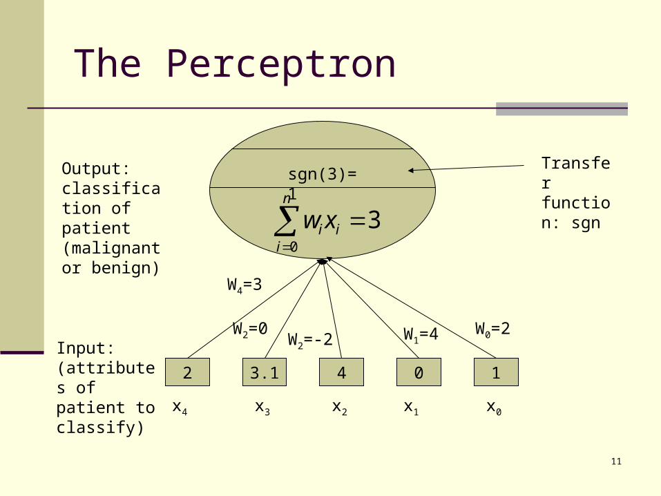
The Perceptron

2 3.1 4 10



W4=3

W2=0W2=-2 W1=4 W0=2

x0x4 x3 x2 x1

30

n

iiixw

sgn(3)=1Transfer function: sgn

12

The Perceptron



2 3.1 4 10

W4=3

W2=0W2=-2 W1=4 W0=2

x0x4 x3 x2 x1

30

n

iiixw

sgn(3)=1

1

13

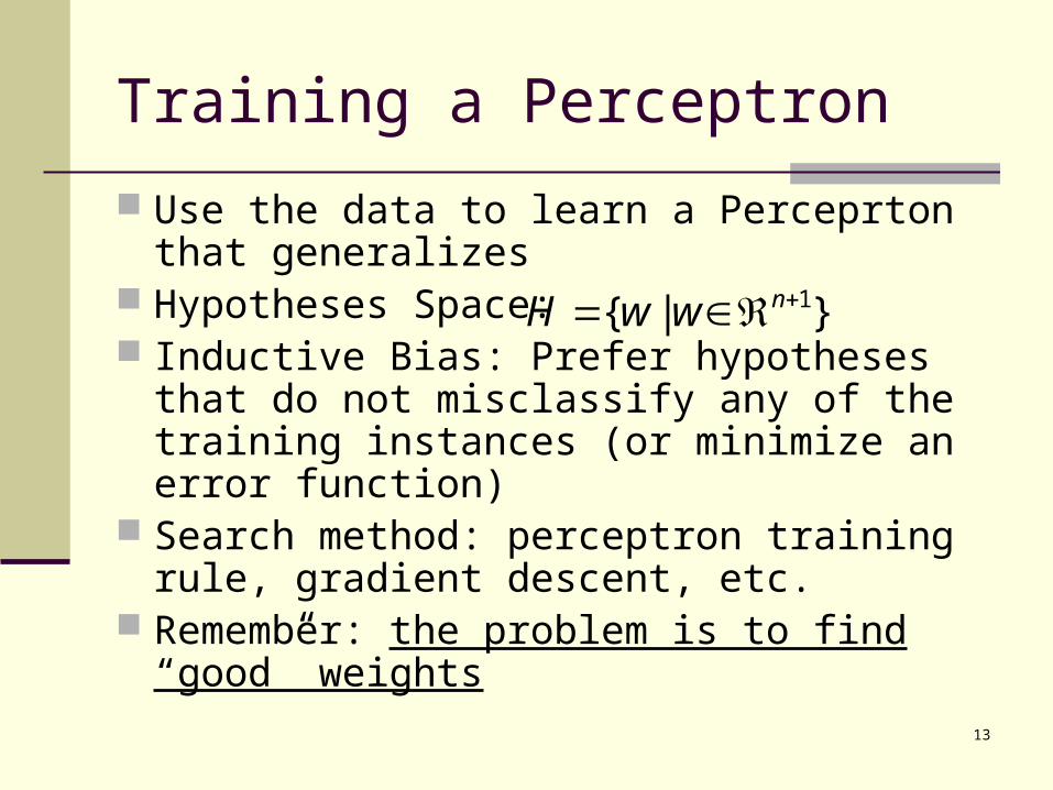
Training a Perceptron

Use the data to learn a Perceprton that generalizes

Hypotheses Space: Inductive Bias: Prefer hypotheses that do not

misclassify any of the training instances (or minimize an error function)

Search method: perceptron training rule, gradient descent, etc.

Remember: the problem is to find “good” weights

}|{ 1 nwwH

14

Training Perceptrons

Start with random weights

Update in an intelligent way to improve them using the data

Intuitively (for the example on the right): Decrease the weights

that increase the sum Increase the weights

that decrease the sum Repeat for all training

instances until convergence

2 3.1 4 10

30 -2 4 2

x0x4 x3 x2 x1

30

n

iiixw

sgn(3)=1

1True Output: -1

15

Perceptron Training Rule

η: arbitrary learning rate (e.g. 0.5)

td : (true) label of the dth example

od: output of the perceptron on the dth example

xi,d: value of predictor variable i of example d

td = od : No change (for correctly classified examples)

ddd

iii

diddi

d

xotww

www

xotw

x

)(

:form vector In

)(

: weightsupdate example

fiedmissclassi eachFor

'

'

,

16

Explaining the Perceptron Training Rule

td = -1, od = 1 : will decrease

td = 1, od = -1 : will increase

2' )( ddddddd xotxwxwxwxw

)sgn( :Output

)( :Rule '

d

ddd

xw

xotww

dxw

dxw

Effect on the output caused by a misclassified example xd

17

Example of Perceptron Training: The OR function

x1

x 2

0 1

1

-1

1 1

1

18


Initial random weights:

Define line:

x1=0.5

Thus:x1

x 2

0 1

1

-1

1 1

1

05.010 12 xx

5.0,1,0

,, 012

wwww

19


Initial random weights:

Defines line:

x1=0.5x1

x 2

0 1

1

-1

1 1

1

05.010 12 xx

x1=0.5

Area where classifier outputs 1

Area where classifier outputs -1

20


x1

x 2

0 1

1

-1

1 1

1

x1=0.5

Only misclassified example x2=1, x1=0, x0 = 1

Area where classifier outputs 1

Area where classifier outputs -1

1,0,1x

21


x1

x 2

0 1

1

-1

1 1

1

x1=0.5

05.010 : LineOld 12 xx


1,0,1x

5.0,1,1

1,0,115.0,1,0

1,0,1))1(1(5.05.0,1,0

)(

weightsUpdate

'

'

'

'

w

w

w

xotww

22


x1

x 2

0 1

1

-1

1 1

1

x1=0.5

1,1,0.5w weights

05.011 :lineNew 12

xx

For x2=0, x1=-0.5

For x1=0, x2=-0.5

So, new line is:

(next slide)


1,0,1x

23


x1

x 2

0 1

1

-1

1 1

1

x1=0.5

05.011 :lineNew 12 xx

-0.5

-0.5

05.011 12 xx

Example correctly classified

after update

24


x1

x 2

0 1

1

-1

1 1

1

-0.5

-0.5

05.011 12 xx

Newly Misclassified example

Next iteration:

5.0,1,1

1,0,015.0,1,1

1,0,0)11(5.05.0,1,1

)(

'

'

'

'

w

w

w

xotww

1,0,0x

25


x1

x 2

0 1

1

-1

1 1

1

-0.5

-0.5

05.011 12 xx

New line: 1x2+1x1-0.5=0

Perfect classification

No change occurs next

26

Analysis of the Perceptron Training Rule Algorithm will always converge within finite

number of iterations if the data are linearly separable.

Otherwise, it may oscillate (no convergence)

27

Training by Gradient Descent

Similar but: Always converges Generalizes to training networks of

perceptrons (neural networks) and training networks for multicategory classification or regression

Idea: Define an error function Search for weights that minimize the error, i.e.,

find weights that zero the error gradient

28

Setting Up the Gradient Descent

Squared Error: td label of dth example, od current output on dth example

Minima exist where gradient is zero:

Dd

dd otwE 2)(2

1)(

Ddd

idd

Dddd

idd

Dddd

i

Dddd

ii

ow

ot

otw

ot

otw

otww

E

)()(

)()(22

1

)(2

1

)(2

1

2

2

29

The Sign Function is not Differentiable

0except everywhere ,0)(

di

dd

i

ow

oo

w

30

Use Differentiable Transfer Functions

Replace

with the sigmoid

)sgn( dxw

))(1)(()(

1

1)(

)(

ysigysigdy

ydsige

ysig

xwsig

y

d

31

Calculating the Gradient

Ddddddd

Dddidddd

Ddd

idddd

Dd i

d

d

ddd

Ddd

idd

Ddd

idd

Ddd

idd

i

xxwsigxwsigotwE

xxwsigxwsigot

xww

xwsigxwsigot

w

xw

xw

xwsigot

xwsigw

ot

xwsigw

ot

ow

otw

E

))(1)(()()(

))(1)(()(

)())(1)(()(

)(

)(

)()(

))(()(

))(()(

)()(

,

32

Updating the Weights with Gradient Descent

Each weight update goes through all training instances

Each weight update more expensive but more accurate

Always converges to a local minimum regardless of the data

When using the sigmoid: output is a real number between 0 and 1

Thus, labels (desired outputs) have to be represented with numbers from 0 to 1

Ddddddd xxwsigxwsigotww

wEww

))(1)(()(

)(

33

Encoding Multiclass Problems

E.g., 4 nominal classes, A, B, C, D

X0 X1 X2 … Class

1 0.4 -1 A

1 9 0.5 A

1 1 3 C

1 8.4 -.8 B

1 -3.4 .2 D

34


Use one perceptron (output unit) and encode the output as follows:

Use 0.125 to represent class A (middle point of [0,.25]) Use 0.375, to represent class B (middle point of [.25,.50]) Use 0.625, to represent class C (middle point of [.50,.75]) Use 0.875, to represent class D (middle point of [.75,1]

The training data then becomes:

X0 X1 X2 … Class

1 0.4 -1 0.125

1 9 0.5 0.125

1 1 3 0.625

1 8.4 -.8 0.365

1 -3.4 .2 0.875

35


Use one perceptron (output unit) and encode the output as follows:

Use 0.125 to represent class A (middle point of [0,.25]) Use 0.375, to represent class B (middle point of [.25,.50]) Use 0.625, to represent class C (middle point of [.50,.75]) Use 0.875, to represent class D (middle point of [.75,1]

To classify a new input vector x:

For two classes only and a sigmoid unit suggested values 0.1 and 0.9 (or 0.25 and 0.75)

DClass asclassify ]1,.75[.)( If

C Class asclassify ]75,.5[.)( If

BClass asclassify ]5,.25[.)( If

A Class asclassify ]25,.0[)( If

xwsig

xwsig

xwsig

xwsig

36

1-of-M Encoding

Assign to class with largest output

x0x4 x3 x2 x1

Output for Class A

Output for Class B

Output for Class C

Output for Class D

37

1-of-M Encoding

E.g., 4 nominal classes, A, B, C, D

X0 X1 X2 … Class A

Class B

Class C

Class D

1 0.4 -1 0.9 0.1 0.1 0.1

1 9 0.5 0.9 0.1 0.1 0.1

1 1 3 0.1 0.1 0.9 0.1

1 8.4 -.8 0.1 0.9 0.1 0.1

1 -3.4 .2 0.1 0.1 0.1 0.9

38

Encoding the Input Variables taking real values (e.g. magnesium level)

Input directly to the Perceptron Variables taking discrete ordinal numerical values

Input directly to the Perceptron (scale linearly to [0,1]) Variables taking discrete ordinal non-numerical values (e.g.

temperature low, normal , high) Assign a number (from [0,1]) to each value in the same

order: Low 0 Normal 0.5 High 1

Variables taking nominal values Assign a number (from [0,1]) to each value (like above) OR,

Create a new variable for each value taking. The new variable is 1 when the original variable is assigned that value, and 0 otherwise (distributed encoding)

39

Feed-Forward Neural Networks

x0x4 x3 x2 x1

Output Layer

Hidden Layer 2

Hidden Layer 1

Input Layer

40

Increased Expressiveness Example: Exclusive OR

x 2

0 1

1

-1

1

1

-1

No line (no set of three weights) can separate the training examples (learn the true function).

x2 x1 x0

w2 w1 w0

41

Increased Expressiveness Examplex 2

0 1

1

-1

1

1

-1

x2 x1 x0

w2,1 w1,1

w0,1

w2,2

w1,2 w0,2

w’1,1 w’2,1

42


0 1

1

-1

1

1

-1

H1

x2 x1

1x0

1 -1

0.5

H2

-1

1 0.5

O

11

X1 X2 Class

0 0 -1

0 1 1

1 0 1

1 1 -1

All nodes have the sign function as transfer function in this example

43


-1

1

1

-1

H1

x2 x1

1x0

1-1

-0.5

H2

-1

1 -0.5

11

X1 X2 C H1 H2 O

T1 0 0 -1 -1 -1 -1

T2 0 1 1 -1 1 1

T3 1 0 1 1 -1 1

T4 1 1 -1 -1 -1 -1

x1

44

From the Viewpoint of the Output Layer

H1 H2

O

11

C H1 H2 O

T1 -1 -1 -1 -1

T2 1 -1 1 1

T3 1 1 -1 1

T4 -1 -1 -1 -1

T1

T3

T2x1

x 2

T4

Mapped By Hidden Layer to:

T1T3

T2

H1

H2

T4

45

From the Viewpoint of the Output Layer

T1

T3

T2x1

x 2

T4

Mapped By Hidden Layer to:

T1T3

T2

H1

H2

T4

•Each hidden layer maps to a new feature space

•Each hidden node is a new constructed feature

•Original Problem may become separable (or easier)

46

How to Train Multi-Layered Networks

Select a network structure (number of hidden layers, hidden nodes, and connectivity).

Select transfer functions that are differentiable.

Define a (differentiable) error function. Search for weights that minimize the error

function, using gradient descent or other optimization method.

BACKPROPAGATION

47

How to Train Multi-Layered Networks

Select a network structure (number of hidden layers, hidden nodes, and connectivity).

Select transfer functions that are differentiable.

Define a (differentiable) error function.

Search for weights that minimize the error function, using gradient descent or other optimization method. x2 x1 x0

w2,1 w1,1

w0,1

w2,2

w1,2 w0,2

w’1,1 w’2,1

Dd

dd otwE 2)(2

1)(

48

BackPropagation

jix

jiw

t

uo

x

ji

ji

u

unit togoing unit frominput

unit tounit from weight

output desired

network in unit every ofoutput

:Notation

or input vect givena For

kunit of Outputs

)1(

unitoutput theis when,))(1(

:Define

uuukkkk

kkkk

woo

kotoo

jijjiji xww :rule weightsUpdate

49

Training with BackPropagation

Going once through all training examples and updating the weights: one epoch

Iterate until a stopping criterion is satisfied The hidden layers learn new features and

map to new spaces

50

Overfitting with Neural Networks

If number of hidden units (and weights) is large, it is easy to memorize the training set (or parts of it) and not generalize

Typically, the optimal number of hidden units is much smaller than the input units

Each hidden layer maps to a space of smaller dimension

51

Avoiding Overfitting : Method 1

The weights that minimize the error function may create complicate decision surfaces

Stop minimization early by using a validation data set Gives a preference to smooth and simple

surfaces

52

Typical Training Curve

Epoch

Error

Real Error or on an independent validation set

Error on Training Set

Ideal training stoppage

53

Example of Training Stopping Criteria

Split data to train-validation-test sets Train on train, until error in validation set is

increasing (more than epsilon the last m iterations), or

until a maximum number of epochs is reached Evaluate final performance on test set

54

Avoiding Overfitting in Neural Networks: Method 2 Sigmoid almost linear around

zero Small weights imply decision

surfaces that are almost linear

Instead of trying to minimize only the error, minimize the error while penalizing for large weights

Again, this imposes a preference for smooth and simple (linear) surfaces

22)(2

1)( wotwE

Dddd

55

Classification with Neural Networks

Determine representation of input: E.g., Religion {Christian, Muslim, Jewish} Represent as one input taking three different

values, e.g. 0.2, 0.5, 0.8 Represent as three inputs, taking 0/1 values

Determine representation of output (for multiclass problems) Single output unit vs Multiple binary units

56


Select Number of hidden layers Number of hidden units Connectivity Typically: one hidden layer, hidden units is a small

fraction of the input units, full connectivity Select error function

Typically: minimize mean squared error (with penalties for large weights), maximize log likelihood of the data

57


Select a training method: Typically gradient descent (corresponds to

vanilla Backpropagation) Other optimization methods can be used:

Backpropagation with momentum Trust-Region Methods Line-Search Methods

Congugate Gradient methods Newton and Quasi-Newton Methods

Select stopping criterion

58

Classifying with Neural Networks

Select a training method: May include also searching for optimal

structure May include extensions to avoid getting stuck

in local minima Simulated annealing Random restarts with different weights

59

Classifying with Neural Networks

Split data to: Training set: used to update the weights Validation set: used in the stopping criterion Test set: used in evaluating generalization

error (performance)

60

Other Error Functions in Neural Networks Minimizing cross entropy with respect to

target values network outputs interpretable as probability

estimates

61

Representational Power

Perceptron: Can learn only linearly separable functions

Boolean Functions: learnable by a NN with one hidden layer

Continuous Functions: learnable with a NN with one hidden layer and sigmoid units

Arbitrary Functions: learnable with a NN with two hidden layers and sigmoid units

Number of hidden units in all cases unknown

62

Issues with Neural Networks

No principled method for selecting number of layers and units Tiling: start with a small network and keep

adding units Optimal brain damage: start with a large

network and keep removing weights and units Evolutionary methods: search in the space of

structures for one that generalizes well No principled method for most other design

choices

63

Important but not Covered in This Tutorial Very hard to understand the classification

logic from direct examination of the weights Large recent body of work in extracting

symbolic rules and information from Neural Networks

Recurrent Networks, Associative Networks, Self-Organizing Maps, Committees or Networks, Adaptive Resonance Theory etc.

64

Why the Name Neural Networks?

Initial models that simulate real neurons to use for classification

Efforts to improve and understand classification independent of similarity to biological neural networks

Efforts to simulate and understand biological neural networks to a larger degree

65

Conclusions

Can deal with both real and discrete domains Can also perform density or probability estimation Very fast classification time Relatively slow training time (does not easily scale to

thousands of inputs) One of the most successful classifiers yet Successful design choices still a black art Easy to overfit or underfit if care is not applied

66

Suggested Further Reading

Tom Mitchell, Introduction to Machine Learning, 1997

Hastie, Tibshirani, Friedman, The Elements of Statistical Learning, Springel 2001

Hundreds of papers and books on the subject

131 Feed-Forward Artificial Neural Networks MEDINFO 2004, T02: Machine Learning Methods for Decision...

Documents

Transcript of 131 Feed-Forward Artificial Neural Networks MEDINFO 2004, T02: Machine Learning Methods for Decision...