1/30: Topic 4.1 – Nested Logit and Multinomial Probit Models Microeconometric Modeling William...
22
1/30: Topic 4.1 – Nested Logit and Multinomial Probit Models Microeconometric Modeling William Greene Stern School of Business New York University New York NY USA 4.1 Nested Logit and Multinomial Probit Models
-
Upload
coleen-holland -
Category
Documents
-
view
219 -
download
1
Transcript of 1/30: Topic 4.1 – Nested Logit and Multinomial Probit Models Microeconometric Modeling William...

1/30: Topic 4.1 – Nested Logit and Multinomial Probit Models
Microeconometric Modeling
William GreeneStern School of BusinessNew York UniversityNew York NY USA
4.1 Nested Logit and Multinomial Probit Models

2/30: Topic 4.1 – Nested Logit and Multinomial Probit Models
Concepts
• Correlation• Random Utility• RU1 and RU2• Tree• 2 Step vs. FIML• Decomposition of Elasticity• Degenerate Branch• Scaling• Normalization• Stata/MPROBIT
Models
• Multinomial Logit• Nested Logit• Best/Worst Nested Logit• Error Components Logit• Multinomial Probit

3/30: Topic 4.1 – Nested Logit and Multinomial Probit Models
Extended Formulation of the MNL Sets of similar alternatives
Compound Utility: U(Alt)=U(Alt|Branch)+U(branch)
Behavioral implications – Correlations within branches
Travel
Private
Public
Air Car Train Bus
LIMB
BRANCH
TWIG

4/30: Topic 4.1 – Nested Logit and Multinomial Probit Models
Correlation Structure for a Two Level Model
Within a branch Identical variances (IIA (MNL) applies) Covariance (all same) = variance at higher level
Branches have different variances (scale factors) Nested logit probabilities: Generalized Extreme Value
Prob[Alt,Branch] = Prob(branch) * Prob(Alt|Branch)

5/30: Topic 4.1 – Nested Logit and Multinomial Probit Models
Probabilities for a Nested Logit Model
k|j k|j
j
Utility functions; (Drop observation indicator, i.)
Twig level : k | j denotes alternative k in branch j
U(k | j) = α +
Branch level U(j) =
Twig level proba
β x
y
( )
( )
( )
k|j k|jk|j K|j
m|j m|jm=1
K|jm=1 m|j m|j
j j
b
exp α +bility : P(k | j) = P =
exp α +
Inclusive value for branch j = IV(j) = log Σ exp α +
exp λ +IV(j)Branch level probability : P(j) =
exp λ
β x
β x
β x
y
B
bb=1
j
+IV(b)
λ = 1 for all branches returns the original MNL model
y

6/30: Topic 4.1 – Nested Logit and Multinomial Probit Models
Model Form RU1
=
=
=
k|j
K|j
m|jm=1
K|j
m|jm=1
Twig Level Probability
exp( )Prob(Choice = k | j)
exp( )
Inclusive Value for the Branch
IV(j) log exp( )
Branch Probability
exp λProb(Branch = j)
β'x
β'x
β'x
j j
B
b bb=1
j
+IV(j)
exp λ +IV(b)
λ = 1 Returns the Multinomial Logit Model
γ'y
γ'y

7/30: Topic 4.1 – Nested Logit and Multinomial Probit Models
Moving Scaling Down to the Twig Level
k|j
j
k|jk|j m|j
m=1j
k|j m|j
m=1j
j j
j
RU2 Normalization
expμ
Twig Level Probability : P
expμ
Inclusive Value for the Branch : IV(j) = log expμ
exp μBranch Probability : P
β x
β x
β x
γ y
B
b bb=1
IV(j)
exp γ y +μ IV(b)

8/30: Topic 4.1 – Nested Logit and Multinomial Probit Models
Higher Level Trees
E.g., Location (Neighborhood) Housing Type (Rent, Buy, House, Apt) Housing (# Bedrooms)

9/30: Topic 4.1 – Nested Logit and Multinomial Probit Models
Estimation Strategy for Nested Logit Models
Two step estimation (ca. 1980s) For each branch, just fit MNL
Loses efficiency – replicates coefficients For branch level, fit separate model, just including y and the
inclusive values in the branch level utility function Again loses efficiency
Full information ML (current) Fit the entire model at once, imposing all restrictions

10/30: Topic 4.1 – Nested Logit and Multinomial Probit Models
MNL Baseline
-----------------------------------------------------------Discrete choice (multinomial logit) modelDependent variable ChoiceLog likelihood function -172.94366Estimation based on N = 210, K = 10R2=1-LogL/LogL* Log-L fncn R-sqrd R2AdjConstants only -283.7588 .3905 .3787Chi-squared[ 7] = 221.63022Prob [ chi squared > value ] = .00000Response data are given as ind. choicesNumber of obs.= 210, skipped 0 obs--------+--------------------------------------------------Variable| Coefficient Standard Error b/St.Er. P[|Z|>z]--------+-------------------------------------------------- GC| .07578*** .01833 4.134 .0000 TTME| -.10289*** .01109 -9.280 .0000 INVT| -.01399*** .00267 -5.240 .0000 INVC| -.08044*** .01995 -4.032 .0001 A_AIR| 4.37035*** 1.05734 4.133 .0000AIR_HIN1| .00428 .01306 .327 .7434 A_TRAIN| 5.91407*** .68993 8.572 .0000TRA_HIN3| -.05907*** .01471 -4.016 .0001 A_BUS| 4.46269*** .72333 6.170 .0000BUS_HIN4| -.02295 .01592 -1.442 .1493--------+--------------------------------------------------

11/30: Topic 4.1 – Nested Logit and Multinomial Probit Models
FIML Parameter Estimates
-----------------------------------------------------------FIML Nested Multinomial Logit ModelDependent variable MODELog likelihood function -166.64835The model has 2 levels.Random Utility Form 1:IVparms = LMDAb|lNumber of obs.= 210, skipped 0 obs--------+--------------------------------------------------Variable| Coefficient Standard Error b/St.Er. P[|Z|>z]--------+-------------------------------------------------- |Attributes in the Utility Functions (beta) GC| .06579*** .01878 3.504 .0005 TTME| -.07738*** .01217 -6.358 .0000 INVT| -.01335*** .00270 -4.948 .0000 INVC| -.07046*** .02052 -3.433 .0006 A_AIR| 2.49364** 1.01084 2.467 .0136AIR_HIN1| .00357 .01057 .337 .7358 A_TRAIN| 3.49867*** .80634 4.339 .0000TRA_HIN3| -.03581*** .01379 -2.597 .0094 A_BUS| 2.30142*** .81284 2.831 .0046BUS_HIN4| -.01128 .01459 -.773 .4395 |IV parameters, lambda(b|l),gamma(l) PRIVATE| 2.16095*** .47193 4.579 .0000 PUBLIC| 1.56295*** .34500 4.530 .0000--------+--------------------------------------------------

12/30: Topic 4.1 – Nested Logit and Multinomial Probit Models
Elasticities Decompose Additively

13/30: Topic 4.1 – Nested Logit and Multinomial Probit Models
+-----------------------------------------------------------------------+| Elasticity averaged over observations. || Attribute is INVC in choice AIR || Decomposition of Effect if Nest Total Effect|| Trunk Limb Branch Choice Mean St.Dev|| Branch=PRIVATE || * Choice=AIR .000 .000 -2.456 -3.091 -5.547 3.525 || Choice=CAR .000 .000 -2.456 2.916 .460 3.178 || Branch=PUBLIC || Choice=TRAIN .000 .000 3.846 .000 3.846 4.865 || Choice=BUS .000 .000 3.846 .000 3.846 4.865 |+-----------------------------------------------------------------------+| Attribute is INVC in choice CAR || Branch=PRIVATE || Choice=AIR .000 .000 -.757 .650 -.107 .589 || * Choice=CAR .000 .000 -.757 -.830 -1.587 1.292 || Branch=PUBLIC || Choice=TRAIN .000 .000 .647 .000 .647 .605 || Choice=BUS .000 .000 .647 .000 .647 .605 |+-----------------------------------------------------------------------+| Attribute is INVC in choice TRAIN || Branch=PRIVATE || Choice=AIR .000 .000 1.340 .000 1.340 1.475 || Choice=CAR .000 .000 1.340 .000 1.340 1.475 || Branch=PUBLIC || * Choice=TRAIN .000 .000 -1.986 -1.490 -3.475 2.539 || Choice=BUS .000 .000 -1.986 2.128 .142 1.321 |+-----------------------------------------------------------------------+| * indicates direct Elasticity effect of the attribute. |+-----------------------------------------------------------------------+

14/30: Topic 4.1 – Nested Logit and Multinomial Probit Models
Testing vs. the MNL
Log likelihood for the NL model Constrain IV parameters to equal 1 with
; IVSET(list of branches)=[1] Use likelihood ratio test For the example:
LogL (NL) = -166.68435 LogL (MNL) = -172.94366 Chi-squared with 2 d.f. = 2(-166.68435-(-172.94366))
= 12.51862 The critical value is 5.99 (95%) The MNL (and a fortiori, IIA) is rejected
15/30: Topic 4.1 – Nested Logit and Multinomial Probit Models
Degenerate Branches
Travel
Fly Ground
Air CarTrain Bus
BRANCH
TWIG
LIMB

16/30: Topic 4.1 – Nested Logit and Multinomial Probit Models
NL Model with a Degenerate Branch
-----------------------------------------------------------FIML Nested Multinomial Logit ModelDependent variable MODELog likelihood function -148.63860--------+--------------------------------------------------Variable| Coefficient Standard Error b/St.Er. P[|Z|>z]--------+-------------------------------------------------- |Attributes in the Utility Functions (beta) GC| .44230*** .11318 3.908 .0001 TTME| -.10199*** .01598 -6.382 .0000 INVT| -.07469*** .01666 -4.483 .0000 INVC| -.44283*** .11437 -3.872 .0001 A_AIR| 3.97654*** 1.13637 3.499 .0005AIR_HIN1| .02163 .01326 1.631 .1028 A_TRAIN| 6.50129*** 1.01147 6.428 .0000TRA_HIN2| -.06427*** .01768 -3.635 .0003 A_BUS| 4.52963*** .99877 4.535 .0000BUS_HIN3| -.01596 .02000 -.798 .4248 |IV parameters, lambda(b|l),gamma(l) FLY| .86489*** .18345 4.715 .0000 GROUND| .24364*** .05338 4.564 .0000--------+--------------------------------------------------

17/30: Topic 4.1 – Nested Logit and Multinomial Probit Models
The Multinomial Probit Model
=
j itj j it i,t,j
1 2 J
U(i,t, j) α + + ' +ε
[ε ,ε ,...,ε ] ~ Multivariate Normal[ , ]
Correlation across choices
Heteroscedasticity
Some restrictions needed for identification
Sufficient : Last row of last row of
β'x γ z
0 Σ
Σ I
One additional diagonal element = 1.

18/30: Topic 4.1 – Nested Logit and Multinomial Probit Models
Multinomial Probit Probabilities
( ,1) ( , ) ( ,1) ( , 1) ( ,1) ( ,1)
1 1 1 ( )
( , ) ( ,1)
( , ) ( ,2)
...
( , ) ( , )
Prob( ) ... ( , ... | )
Requires (J-1)-variate multivariate normal integration with a full c
U i U i J U i U i J U i U i
J J J j
U i j U i
U i j U i
U i j U i J
event d
1
1 1
ovariance matrix.
The GHK simulator uses simulation to compute these probabilities accurately
1using a simulation of the form Prob( ) [ ( )].
= sequences of random N[0,1] draw
R J
krr j
kr
event h wR
w s using a simulator.

19/30: Topic 4.1 – Nested Logit and Multinomial Probit Models
The problem of just reporting coefficients
Stata: AIR = “base alternative” Normalizes on CAR
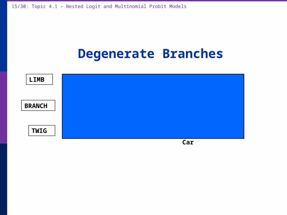
20/30: Topic 4.1 – Nested Logit and Multinomial Probit Models
+---------------------------------------------+| Multinomial Probit Model || Dependent variable MODE || Number of observations 210 ||| Log likelihood function -184.7619 | Not comparable to MNL| Response data are given as ind. choice. |+---------------------------------------------++--------+--------------+----------------+--------+--------+|Variable| Coefficient | Standard Error |b/St.Er.|P[|Z|>z]|+--------+--------------+----------------+--------+--------+---------+Attributes in the Utility Functions (beta) GC | .10822534 .04339733 2.494 .0126 TTME | -.08973122 .03381432 -2.654 .0080 INVC | -.13787970 .05010551 -2.752 .0059 INVT | -.02113622 .00727190 -2.907 .0037 AASC | 3.24244623 1.57715164 2.056 .0398 TASC | 4.55063845 1.46158257 3.114 .0018 BASC | 4.02415398 1.28282031 3.137 .0017---------+Std. Devs. of the Normal Distribution. s[AIR] | 3.60695794 1.42963795 2.523 .0116 s[TRAIN]| 1.59318892 .81711159 1.950 .0512 s[BUS] | 1.00000000 ......(Fixed Parameter)....... s[CAR] | 1.00000000 ......(Fixed Parameter).......---------+Correlations in the Normal Distribution rAIR,TRA| .30491746 .49357120 .618 .5367 rAIR,BUS| .40383018 .63548534 .635 .5251 rTRA,BUS| .36973127 .42310789 .874 .3822 rAIR,CAR| .000000 ......(Fixed Parameter)....... rTRA,CAR| .000000 ......(Fixed Parameter)....... rBUS,CAR| .000000 ......(Fixed Parameter).......
Correlation Matrix for
Air, Train, Bus, Car
1 .305 .404 0
.305 1 .370 0
.404 .370 1 0
0 0 0 1
Multinomial Probit Model

21/30: Topic 4.1 – Nested Logit and Multinomial Probit Models
Multinomial Probit Elasticities+---------------------------------------------------+| Elasticity averaged over observations.|| Attribute is INVC in choice AIR || Effects on probabilities of all choices in model: || * = Direct Elasticity effect of the attribute. || Mean St.Dev || * Choice=AIR -4.2785 1.7182 || Choice=TRAIN 1.9910 1.6765 || Choice=BUS 2.6722 1.8376 || Choice=CAR 1.4169 1.3250 || Attribute is INVC in choice TRAIN || Choice=AIR .8827 .8711 || * Choice=TRAIN -6.3979 5.8973 || Choice=BUS 3.6442 2.6279 || Choice=CAR 1.9185 1.5209 || Attribute is INVC in choice BUS || Choice=AIR .3879 .6303 || Choice=TRAIN 1.2804 2.1632 || * Choice=BUS -7.4014 4.5056 || Choice=CAR 1.5053 2.5220 || Attribute is INVC in choice CAR || Choice=AIR .2593 .2529 || Choice=TRAIN .8457 .8093 || Choice=BUS 1.7532 1.3878 || * Choice=CAR -2.6657 3.0418 |+---------------------------------------------------+
+---------------------------+| INVC in AIR || Mean St.Dev || * -5.0216 2.3881 || 2.2191 2.6025 || 2.2191 2.6025 || 2.2191 2.6025 || INVC in TRAIN || 1.0066 .8801 || * -3.3536 2.4168 || 1.0066 .8801 || 1.0066 .8801 || INVC in BUS || .4057 .6339 || .4057 .6339 || * -2.4359 1.1237 || .4057 .6339 || INVC in CAR || .3944 .3589 || .3944 .3589 || .3944 .3589 || * -1.3888 1.2161 |+---------------------------+
Multinomial Logit

22/30: Topic 4.1 – Nested Logit and Multinomial Probit Models
Not the Multinomial Probit ModelMPROBIT
This is identical to the multinomial logit – a trivial difference of scaling that disappears from the partial effects. (Use ASMProbit for a true multinomial probit model.)