13 Searching the Web with the SVD

13.1 Information retrieval

Over the last 20 years the number of internet users has grown exponentially with time; seeFigure 1. Trying to extract information from this exponentially growing resource of materialcan be a daunting task. Information retrieval (IR) is an interdisciplinary science, which isconcerned with automated storage and retrieval of documents.

1988 1991 1994 1997 20000

1

2

3

4

5

6

7

8x 10

7

Num

ber

of In

tern

et U

sers

Figure 1: Internet data obtained from the website http://www.isc.org/ds/host-count-history.html.

IR systems are used to handle extremely large sets of digital data and help reduce in-formation overload.1 One of the largest digital data sets is the Internet with more than 20billion web pages. In order to extract a small subset of useful information from this hugedigital data set requires a web search engine. The grandfather of search engines, which wasreally not a search engine, was called Archie and was created in 1990 by Peter Deutsch, AlanEmtage, and Bill Wheelan. After Archie, followed a whole array of search engines; WorldWide Web Wanderer (1993), Excite (1993), Yahoo (1994), Infoseek (1994), Lycos (1994),AltaVista (1995), and Google (1997) to name a few. In this lecture you will learn how tocreate a web search engine using a vector space model.

1The term Information overload was originated in 1970 by Alvin Toffler in his book Future Shock. Itrefers to having too much information in order to make a decision.

1

13.2 A vector space model

Central for the discussion to follow are the term-by-document matrices. A term-by-documentmatrix A = [ai,j] is constructed by letting the entries ai,j represent the frequency of the termi in document j. We are interested in the situation when the documents are web pages,however, the method described can be applied to other documents as well, such as letters,books, phone calls, etc.

Doc1

Math, Math, Calculus, Algebra

Doc2

Math, Club, Advisor

Doc3

Computer, Club, Club

Doc4

Ball, Ball, Ball, Math Algebra

Advisor

Algebra

Ball

Calculus

Club

Computer

Math

Doc1 Doc2 Doc3 Doc4

0 1 0 0

1 0 0 1

0 0 0 3

1 0 0 0

0 1 2 0

0 0 1 0

2 1 0 1

Figure 2: The term-by-document matrix for Example 13.1.

Example 13.1. Consider the term-by-document matrix of Figure 2. The words (=terms)of interest are Advisor, Algebra, Ball, Calculus, Club, Computer, and Math. There are fourdocuments or web pages. Therefore the term-by-document matrix is of size 7 × 4. Noticethat a3,4 = 3 shows that in document 4, the term Ball occurs 3 times, and a5,2 = 1 indicatesthat in document 2 the term Club occurs once. Term-by-document matrices are inherentlysparse, since every word does not normally appear in each document. 2

Example 13.2. The term-by-document matrix, Hypatia, of the web server of the mathe-matics department at the University of Rhode Island is of size 11, 390× 1, 265 with 109, 056non-zero elements. The matrix is sparse because only a small fraction of its entries are non-vanishing (less than 1%). The Matlab command spy can be used to visualize the sparsitystructure of a matrix. Figure 3 depicts the sparsity structure of Hypatia. 2

How does one search (i.e., query) a system to determine which documents contain thesearch element? A simple approach would be to return the nonvanishing elements of the rowof the term-by-document matrix that match the search element.

2

0 200 400 600 800 1000 1200

0

2000

4000

6000

8000

10000

nz = 109056

Figure 3: Sparsity pattern of the 11, 390× 1, 265 term-by-document matrix Hypatia. This matrixis available at http://www.math.uri.edu/∼jbaglama/software/hypatia.gz

Example 13.3. We would like to search for Club using the term-by-document matrix ofFigure 2. The row corresponding to Club in this matrix is [ 0 1 2 0 ]. This shows thatdocuments 2 and 3 contain the word Club.

Consider instead searching for the term Algebra. The row of the term-by-documentmatrix corresponding to Algebra is [ 1 0 0 1 ]. This identifies the documents 1 and 4. 2

However, for very large matrices the approach of Examples 13.2 and 13.3 to identifydocuments is not practical. A reason for this is that there are many ways to express a givenconcept (club, organization, society) and the literal terms in a user’s query may not matchthose of relevant documents. For this reason, the number of documents identified may be toosmall. On the other hand, many words have multiple meanings (club, stick) and thereforeterms in a user’s query will literally match terms in irrelevant documents. The number ofdocuments identified therefore may be much too large. Moreover, typically one does notonly want to know about matches, but one would like to know the most relevant documents,i.e., one would like to rank the documents according to relevance.

3

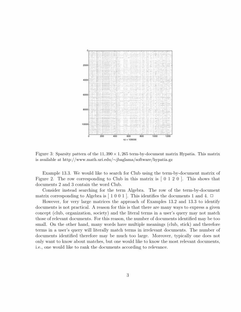
Example 13.4. Consider the matrix A from Figure 2, and a query vector for Club,

A =

0 1 0 01 0 0 10 0 0 31 0 0 00 1 2 00 0 1 02 1 0 1

q =

0000100

AdvisorAlgebraBallCalculus

← ClubComputerMath

(1)

The angle θj between the column of A(:, j) of a term-by-document matrix and the queryvector q can be computed by

cos(θj) =qT A(:, j)

‖q‖‖A(:, j)‖, j = 1, 2, , . . . . (2)

Notice that when q is identical with the jth column of A, the angle between q and thiscolumn vanishes and the cosine of this angle is one. Thus, a large value of cos(θj) suggeststhat document j may be relevant.

In particular, for the term-by-document matrix (1) and query vector q for Club we have,

cos(θ1) = 0, cos(θ2) = 0.5774, cos(θ3) = 0.8944, cos(θ4) = 0. (3)

This shows that document 3 is the best match. 2

At this stage of the development of the vector space model for a search engine, usingvectors and matrices does not seem different from simply returning the row of the term-by-document matrix that matches a term, such as Club. However, it will soon become evidentwhy the Singular Value Decomposition (SVD) is needed.

Let us look at Example 13.1 visually in a two-dimensional plot. In order to be able to dothis, we need to project our data into a two-dimensional space. The SVD of the term-by-document matrix A helps us to determine this mapping. Recall that the SVD of a matrixA ∈ Rm×n with m ≥ n is given by

A = UΣV T , (4)

whereU = [u1, u2, . . . , um] ∈ Rm×m and V = [v1, v2, . . . , vn] ∈ Rn×n

are orthogonal and the diagonal entries of

Σ = diag[σ, σ2, . . . , σn] ∈ Rm×n

4

satisfy σ1 ≥ σ2 ≥ · · · ≥ σn ≥ 0. In applications of the SVD to document retrieval, thecolumns uj of U commonly are referred to as term vectors and the columns vj of V asdocument vectors.

The decomposition (4) can be expressed in terms of the columns of U and V explicitly,

A =n∑

j=1

σjujvTj . (5)

It is easily verified that ‖ujvTj ‖ = 1, see Exercise 13.1, and it follows that

‖σjujvTj ‖ = σj.

The decrease of the σj with increasing j suggests that it may be possible to approximate Aby the matrix

Ak =k∑

j=1

σjujvTj , (6)

determined by ignoring the last n− k terms in the sum (5). Let

Uk = [u1, u2, . . . , uk] ∈ Rm×k, Vk = [v1, v2, . . . , vk] ∈ Rn×k,

andΣk = diag[σ1, σ2, . . . , σk] ∈ Rk×k.

ThenAk = UkΣkV

Tk . (7)

The projection of the scaled documents onto a k-dimensional space is given by

VkΣk = AT Uk, (8)

see Exercise 13.2, and, similarly, the projection of the scaled terms onto a k-dimensionalspace can be expressed as

UkΣk = AVk. (9)

In particular, we can determine a two-dimensional plot of the terms and documents by usingthe first two columns of UkΣk and VkΣk.

Example 13.5. Regard Figure 4, which shows the two-dimensional projection of the termsand documents of Example 13.1. Let ej = [0, . . . , 0, 1, 0, . . . , 0]T denote the jth axis vector.The point

eT5 U2Σ2 = (σ1u1,5, σ2u2,5) = (−0.2897, 2.0005)

5

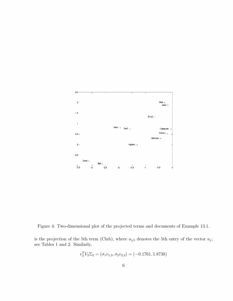
Figure 4: Two-dimensional plot of the projected terms and documents of Example 13.1.

is the projection of the 5th term (Club), where uj,5 denotes the 5th entry of the vector uj;see Tables 1 and 2. Similarly,

eT3 V2Σ2 = (σ1v1,3, σ2v2,3) = (−0.1761, 1.8738)

6

x - coordinates y - coordinatesTerms σ1u1 σ2u2

Documents σ1v1 σ2v2

Table 1: Data for Example 13.5.

σ1u1 σ2u2 σ1v1 σ2v2

−0.1911 0.5194 −1.5889 0.7502−1.3185 −0.0100 −0.6821 1.3144−2.6205 −0.9194 −0.1761 1.8738−0.4450 0.2965 −3.1187 −0.7755−0.2897 2.0005−0.0493 0.7405−1.9546 0.8059

Table 2: Data for Example 13.5.

is the projection of the 3rd document. The projections of the 5th term and 3rd documentare close, which indicates that Doc3 is likely to be a relevant document when we search forClub, in agreement with the discussion above.

However, if we search for Algebra (the 2nd term), then it is not so obvious from Figure 4which document is most relevant. In order find out, we project the query vector for Algebra(q = [0 1 0 0 0 0 0 ]T ) onto the document space. The scaled projection of the query vectoris given by

q(p) = qT Uk.

A comparison with equation (8) shows that the query vector q is projected the same way asthe documents, i.e., the query vector can be thought of as a column of A, i.e., as anotherdocument. If the angle between the vector q(p) and the projected document is small, thenthe document may contain information related to the query.

Figure 5 displays the projected query vector q(p) for Algebra along with plots of theprojected terms and documents. Note that Algebra does not appear in Doc2 in Example13.1, however, Figure 5 shows the angle between q(p) and the projection of Doc2 to be smallerthan 90o. This indicates that Doc2 may be somewhat relevant to Algebra.

Doc2 contains the words Club, Math, and Advisor, and Doc4 and Doc1 contain thewords Math and Algebra. All three documents contain the word Math, and therefore thedocuments may be relevant to the query. Hence, Doc2 could be relevant. Also, notice that

7

Figure 5: Two-dimensional plot of the projected query vector q(p) for Algebra and of theprojected terms and documents of Example 13.1.

Doc3 does not contain the words Math and Algebra, which indicates that this document isunrelated to the query. In fact, the angle between the query vector for Algebra and Doc3 inFigure 5 is almost 90o. 2

Literally matching terms in documents with a query does not always yield clear answers.A better approach is to match a query with the meaning of a document. Latent SemanticIndexing (LSI) does just that. It overcomes the problems of lexical matching by usingstatistically derived quantities instead of individual words for matching.

13.3 Latent semantic indexing (LSI)

Latent semantic indexing examines the whole document collection to determine which doc-uments contain similar words. LSI considers documents that have words in common to besemantically close, and documents with few words in common to be semantically distant.

Let Ak be the rank k approximation (6) of A. Working with Ak instead of A has severaladvantages. Since the small terms in the expansion (5) are neglected the important infor-mation, which is represented by the first terms in the expansion, is now easier accessible.Moreover, we can store Ak in factored form (7) without explicitly forming the elements ofAk. For large matrices A, storage of Ak in this manner typically requires much less computer

8

memory than storage of the matrix A. We remark that there are methods for computingthe matrices Uk, Vk, and Σk without forming A; only matrix-vector products with A and AT

have to be evaluated.

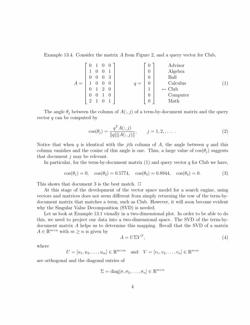
Figure 6: Singular values of the 11, 390× 1, 265 term-by-document matrix Hypatia.

The value of k in Ak is typically chosen experimentally. Even for a very large numberof documents, k = 100 often gives acceptable results. Figure 6 illustrates the magnitude ofthe singular values of the large term-by document matrix Hypatia. Notice that the singularvalues σj decrease to zero very quickly, and a choice of k = 100 would be acceptable. Weremark that choosing k very large does not always result in better answers to queries. Thereason for this is that increasing k increases the search space. The added data is associatedwith small singular values and does not always contain relevant information.

LSI works with the matrix Ak instead of with A. Specifically, one determines the anglebetween the query vector q and every column of Ak. These angles can be computed similarlyas the angles (2). Thus, replacing A by Ak in (2) yields

cos(θj) =qT Akej

‖q‖ ‖Akej‖=

(qT Uk)(ΣkVTk ej)

‖q‖ ‖ΣkV Tk ej‖

, j = 1, 2, . . . , k, (10)

where ej denotes the jth axis vector. Note that qT Uk and ΣkVk are projections of the queryvector and document vectors into k-dimensional spaces; cf. (8).

9

Now returning to Example 13.1 and using equation (10) with k = 2 for LSI, we obtainthe following results. For Club, we have

cos(θ1) = 0.4109, cos(θ2) = 0.7391, cos(θ3) = 0.7947, cos(θ4) = −0.1120,

which gives the ordering Doc3, Doc2, Doc1, and Doc4 of the documents, with Doc3 beingthe most relevant and Doc4 the least relevant document. The query vector for Algebra yields

cos(θ1) = 0.3323, cos(θ2) = 0.1666, cos(θ3) = 0.0306, cos(θ4) = 0.3593,

which determines the ordering Doc4, Doc1, Doc2, and Doc3. Notice that the cosine of theangle between Algebra and Doc3 is close to zero. This indicates that Doc3 is irrelevant forthe query. The angles reveal that Doc2 has some connection to Algebra.

Finally, we note that weighting of the terms in a term-by-document matrix can affectquery results significantly. Documents that have many words or repeat the same word manytimes are erroneously given a high ranking without term weighting. The following sectiondiscusses this topic.

13.4 Term weighting

The weighting of the terms in a term-by-document matrix A can be carried out as follows.Set

ai,j = gi · ti,j · dj,

where gi is the global weight of the ith term, ti,j is the local weight of the ith term in the jthdocument, and dj is the normalization factor for document j. We will define term frequencyfi,j as the number of times the ith term appears in the jth document.

Local weighting depends only on the term within a document and not the occurrenceof the term in other documents. Global weighting seeks to give a value to each term,depending on the occurrences of the term in all documents. For instance, global weightingis used to correct for differences in document lengths. In the tables below, n is the numberof documents.

10

ti,j Local weighting schemeχ(fi,j) 1 if the ith term is in the jth document and 0 otherwise

fi,j Frequency of the ith term in the jth documentThis weighting is used in Example 13.1.

log(fi,j + 1) Logarithmic frequency to reduce the effects of large term frequency(most used local weighting scheme)

Table 3: Examples of local weighting schemes.

gi Global weighting schemes1 None

log( nPnk=1 χ(fi,k)

) Inverse document frequency (IDF), emphasizes rare words

(most used global weighting scheme)Pnk=1 fi,kPn

k=1 χ(fi,k)GFIDF

1 +∑n

j=1pi,j ·log(pi,j)

log(n), pi,j =

fijPnk=1 fi,k

Entropy, gives higher weights for terms with low frequency

Table 4: Examples of global weighting schemes.

Exercises

Exercise 13.1: Let u and v be unit vectors. Show that ‖uvT‖ = 1.

Exercise 13.2: Show the formulas (8) and (9).

Exercise 13.3:a) Reproduce Figure 4.b) Query for the term Calculus and produce a plot analogous to Figure 5.

Exercise 13.4:a) Use the local weighting scheme ti,j = log(fij + 1) (logarithmic frequency) for Example13.1 and produce a two-dimensional plot of the terms and documents similar to Figure 4.b) Query for the term Calculus and produce a plot similar to Figure 5.

Exercise 13.5:a) Use the global weighting scheme log( nPn

k=1 χ(fi,k)) (IDF) for Example 13.1 and produce a

two dimensional plot of the terms and documents similar to Figure 4.b) Query for the term Calculus and produce a plot similar to Figure 5.

11

dj Normalization schemes1 None√∑n

k=1(gk · tk,j)2 Cosine normalization(most used normalization scheme)

Table 5: Examples of normalization schemes.

Exercise 13.6:a) Use both the local weighting scheme ti,j = log(fij + 1) (logarithmic frequency) andthe global weighting scheme log( nPn

k=1 χ(fi,k)) (IDF) for Example 13.1 and produce a two-

dimensional plot of the terms and documents similar to Figure 4.b) Query for the term Calculus and produce a plot similar to Figure 5.

Exercise 13.7: Which was the best method, no weighting, local weighting only, globalweighting only, or both local and global weighting? Repeat your searches with a query vectorfor Calculus and Algebra. What happens? What happens when you query for Calculus andBall?

13.5 Project

We will investigate the LSI search engine method for a small set of FAQ for MATLAB. Inthe directory http://www.math.uri.edu/∼/jbaglama/faq/ there are 68 frequently askedquestions about MATLAB. The questions are in individual text files (i.e., documents)

http://www.math.uri.edu/∼/jbaglama/faq/q1.txthttp://www.math.uri.edu/∼/jbaglama/faq/q2.txt

......

http://www.math.uri.edu/∼/jbaglama/faq/q68.txt

The file http://www.math.uri.edu/∼/jbaglama/faq/documents.txt contains a listof the above documents. The file http://www.math.uri.edu/∼/jbaglama/faq/terms.txtcontains the list of all relevant terms in alphabetical order. There are 1338 terms. Thefile http://www.math.uri.edu/∼/jbaglama/faq/matrix.txt contains the entries of the1338×68 term-by-document matrix. The file matrix.txt was created from the alphabeticallist of terms and the sequential ordering of the questions. The first couple lines of the filematrix.txt are:%term by document matrix for FAQ1338 68 2374

12

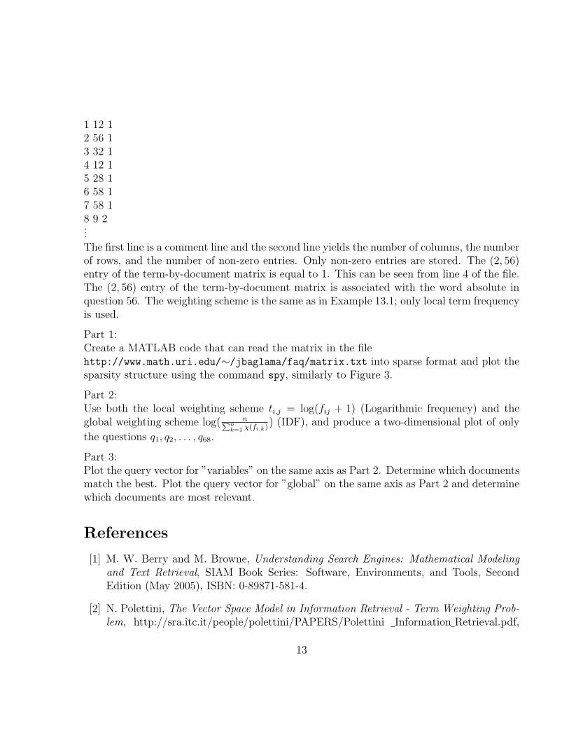
1 12 12 56 13 32 14 12 15 28 16 58 17 58 18 9 2...The first line is a comment line and the second line yields the number of columns, the numberof rows, and the number of non-zero entries. Only non-zero entries are stored. The (2, 56)entry of the term-by-document matrix is equal to 1. This can be seen from line 4 of the file.The (2, 56) entry of the term-by-document matrix is associated with the word absolute inquestion 56. The weighting scheme is the same as in Example 13.1; only local term frequencyis used.

Part 1:Create a MATLAB code that can read the matrix in the filehttp://www.math.uri.edu/∼/jbaglama/faq/matrix.txt into sparse format and plot thesparsity structure using the command spy, similarly to Figure 3.

Part 2:Use both the local weighting scheme ti,j = log(fij + 1) (Logarithmic frequency) and theglobal weighting scheme log( nPn

k=1 χ(fi,k)) (IDF), and produce a two-dimensional plot of only

the questions q1, q2, . . . , q68.

Part 3:Plot the query vector for ”variables” on the same axis as Part 2. Determine which documentsmatch the best. Plot the query vector for ”global” on the same axis as Part 2 and determinewhich documents are most relevant.

References

[1] M. W. Berry and M. Browne, Understanding Search Engines: Mathematical Modelingand Text Retrieval, SIAM Book Series: Software, Environments, and Tools, SecondEdition (May 2005), ISBN: 0-89871-581-4.

[2] N. Polettini, The Vector Space Model in Information Retrieval - Term Weighting Prob-lem, http://sra.itc.it/people/polettini/PAPERS/Polettini Information Retrieval.pdf,

13

2004.

14