13 Categorical data

First of all, a brief reminder of your first encounter with categorical data.

You have already looked at tests of association of categorical data.

Example Gender and smoking

Suppose we are interested in whether there is an association between genderand smoking in the cotton industry? (Well, why not?)

SmokerYes No

Male 2059 857 2916Gender

Female 1130 1373 25033189 2230 5419

Can you remember how to test for an association between gender and smok-ing?

You used one of two statistics: either Pearson’s statistic or the likelihoodratio statistic.

The former is

P =∑i,j

(Oij − Eij)2

Eij

whereOij is the observed number in cell (i, j) and Eij is the expected number.

The likelihood ratio statistic is

Λ = 2r∑

i=1

c∑j=1

nij log

(nijn

ni.n.j

)

where nij is the number in cell (i, j), ni. is the ith row total and n.j is thejth column total. Both statistics have χ2(r−1)(c−1) distributions.To carry out a Pearson test of association between gender and smoking, firstcalculate the Eij.

Eij =(ith row total)× (jth column total)

overall total.

236

The Eij are given in braces in the table below.

SmokerYes No

Male 2059 857 2916(1716.02) (1199.98)

GenderFemale 1130 1373 2503

(1472.98) (1030.02)3189 2230 5419

Then calculate

P =∑i,j

(Oij −Eij)2

Eij

= 361.

This is highly significant against χ2(1) and we reject the null hypothesis ofno association between gender and smoking.

237

13.1 Testing for heterogeneity

There is another situation in which you might want a test of association.Consider the following small study involving 60 consecutive deliveries in ahospital obstetrics ward. The outcome of interest was whether there is a linkbetween babies developing colic and the mother having a spinal painkiller(or epidural). The results are in the table below.

EpiduralYes No

Yes 20 12 32Colic

No 10 18 2830 30

Can you see why this is different from the previous example?

It is different because one of the variables has its marginal totals pre-selected.The investigator has deliberately given 30 epidurals out of a total of 60. Doesthis affect the analysis?A general statement of this situation is:

Take n1 individuals from population 1, and n2 from population2. For each of them an observation is recorded, in the simplestcase, say, a binary observation 1 or 0. Then the correspondingcontingency table will be as below.

Population1 2

1 r1 r2Characteristic

0 n1 − r1 n2 − r2n1 n2

Clearly r1 and r2 are observations on independent random variables R1 andR2.

i.e.

R1 ∼ B(n1, θ1), R2 ∼ B(n2, θ2),

238

and the hypothesis of no association between population and response maybe written

H0 : θ1 = θ2.

The likelihood function is

L(θ1, θ2) =

(n1r1

)θr11 (1− θ1)

n1−r1

(n2r2

)θr22 (1 − θ2)

n2−r2 ,

giving a log-likelihood

l(θ1, θ2) = r1 log θ1 + (n1 − r1) log (1 − θ1) + log(n1r1

)+r2 log θ2 + (n2 − r2) log (1 − θ2) + log

(n2r2

).

∂l

∂θ1=

r1θ1−n1 − r11 − θ1

andθ̂1 =

r1n1.

Similarly

θ̂2 =r2n2,

and, under H0 : θ1 = θ2 = θ,

θ̂ =r1 + r2n1 + n2

.

The likelihood ratio statistic is

Λ = 2

[supθ∈Θ

l(θ)− supθ∈Θ0

l(θ)

],

so, in this case, Λ is given by

2∑2

i=1

[ri log

(rini

)+ 2(ni − ri) log

((ni−ri)

ni

)]−2(r1 + r2) log

((r1+r2)

n

)− 2 (n− (r1 + r2)) log

((n−(r1+r2))

n

),

where n = n1 + n2.

We saw before that the likelihood ratio statistic for contingency tables hadthe form

Λ′ = 2r∑

i=1

c∑j=1

nij log

(nijn

ni.n.j

).

239

In the notation used here,

n11 = r1, n12 = r2,, n21 = n1 − r1, n22 = n2 − r2,

so that

n1. = r1 + r2, n2. = n − (r1 + r2), n.1 = n1, n.2 = n2.

After a little manipulation, we see that

Λ = Λ′.

Thus the test statistic is calculated in exactly the same way as before. Wemay either use the likelihood ratio statistic or the Pearson statistic, since thetwo are asymptotically equivalent.

240

13.2 The odds ratio

We used, as a straightforward reminder of the χ2-test, some data on genderand smoking for workers in the cotton industry in 1973, and we found ahighly significant association.

But the analysis did not tell us whether men tended to be heavier smokersthan women or vice versa. We had to look at the table itself for that − whichwas pretty easy in this case.

The next thing we are going to do is derive an alternative to the χ2-test.I doing this we shall derive a statistic which will tell us the nature of theassociation.

For a 2× 2 table, under the null hypothesis H0 : θAB = θAθB , we have

θAB × θAB = θAB × θAB

or

ψ =θABθABθABθAB

= 1.

ψ is called the odds ratio.It is easy to see why. The odds of an event happening is the ratio of theprobability of it happening to the probability of it not happening. Re-writethe odds ratio as

ψ =θAB/θABθAB/θAB

and the numerator is the odds on level A in preference to not-A for anindividual at level B; the denominator is the odds on level A in preference tonot-A for an individual at level not-B. For the case of no association, ψ = 1.

The odds ratio can be estimated by

ψ̂ =OAB/OAB

OAB/OAB

,

where the observed numbers in the cells have been used.

241

Example Gender and smoking

The table for the cotton workers is

SmokerYes No

Male 2059 857Gender

Female 1130 1373

and the corresponding estimate of the odds ratio is

ψ =2059 × 1373

1130 × 857= 2.92,

which seems to be somewhat larger than 1.

You can interpret this as ‘the odds of a man in the cotton industry turningout to be a smoker are 2.92 times those of a woman’, or equivalently, ‘theodds of a woman in the cotton industry turning out to be a non-smoker are2.92 times those of a man’.

Example Epidurals and colic

What about our example with fixed marginal totals?We are asking the question ‘are 20/30 and 12/30 close or not? We mightjust as well ask the same question about the odds of 20:10 and 12:18, or, ingeneral, θ1 : (1 − θ1) and θ2 : (1− θ2). The odds ratio is

ψ =θ1(1 − θ2)

θ2(1 − θ1)

which takes the value 1 under H0 : θ1 = θ2. This is estimated as

ψ̂ =r1(n2 − r2)

r2(n1 − r1)=

20 × 18

10 × 12= 3.00.

It looks as if babies whose mothers have epidurals have three times the oddsof developing colic.

Once again, although the arguments are different in the two types of table,the odds ratio is a sensible thing to look at and is constructed in exactly thesame way.

242

Having said this, the odds ratio is not terribly useful to us unless we candetermine how far from 1 the estimate ψ̂ can be before we can conclude thatit is significantly far from 1.

As we shall shortly see, it turns out that log ψ̂, the so-called log-odds-ratio,has the properties that, under H0 : θ1 = θ2,

E(log ψ̂

)� 0,

V(log ψ̂

)�

∑1/(observed),

and, furthermore, the test statistic log ψ̂ has approximately a normal distri-bution.

Example Gender and smoking

For the cotton workers, ψ̂ = 2.92 and log ψ̂ = 1.07.

The variance of the log-odds-ratio statistic is

V(log ψ̂

)�

1

2059+

1

1373+

1

1130+

1

857= 0.003266.

So √log ψ̂ � 0.057

andlog ψ̂ − E

(log ψ̂

)√V(log ψ̂

) �1.07

0.057= 18.8.

Sincelog ψ̂ −E

(log ψ̂

)√V(log ψ̂

) D→ N(0, 1),

this is highly significant.

Proof of asymptotic normality

Consider the general 2 × 2 table

B BA a bA c d

243

and let θ1 = P (A | B), θ2 = P (A | B) and let the log-odds-ratio be

ψ = log

(θ1(1− θ2)

θ2(1− θ1)

).

If we write the log-odds of A given B as

ω = log

(θ2

1 − θ2

),

then

ω + ψ = log

(θ1

1 − θ1

)and, re-arranging,

θ1 =eω+ψ

1 + eω+ψ, θ2 =

eω

1 + eω

The likelihood is, therefore,

L(ω,ψ) =

(eω+ψ

1 + eω+ψ

)a(1

1 + eω+ψ

)c( eω

1 + eω

)b( 1

1 + eω

)d

and the log-likelihood, l(ω,ψ), is

a(ω + ψ) + bω − (a+ c) log(1 + eω+ψ

)− (b+ d) log (1 + eω ) .

∂l

∂ψ= a−

(a+ c)eω+ψ

1 + eω+ψ= 0,

∂l

∂ω= a+ b−

(a+ c)eω+ψ

1 + eω+ψ−

(b+ d)eω

1 + eω= 0.

Substitution results in

b−(b+ d)eω

1 + eω= 0 ⇒ eω =

b

d.

Similarly

eω+ψ =a

c⇒ eψ =

ad

bc.

∂2l

∂ψ2 = −(a+ c)∂

∂ψ

(1 −

1

1 + eω+ψ

)= −

(a+ c)

(1 + eω+ψ)2,

244

∂2l

∂ω2= −

(a+ c)

(1 + eω+ψ)2−

(b+ d)

(1 + eω )2,

∂2l

∂ω∂ψ= −

(a+ c)

(1 + eω+ψ)2.

Now substitute for eω+ψ and eω and

∂2l

∂ψ2 =∂2l

∂ω∂ψ= −

ac

a+ c,

∂2l

∂ω2= −

ac

a+ c−

bd

b+ d.

The observed information is, therefore,

J =

(ac/(a+ c) ac/(a+ c)ac/(a+ c) ac/(a+ c) + bd/(b+ d)

).

detJ =abcd

(a+ c)(b+ d)

giving

(J−1)ψψ =

(ac

a+ c+

bd

b+ d

)(a+ c)(b+ d)

abcd

=1

a+

1

b+

1

c+

1

d.

From the result for the asymptotic distribution of a maximum likelihoodestimator, we have

ψ̂D→ N

(E(ψ̂), 1/I(ψ)

).

Since J(ψ̂)P→ I(ψ), ψ̂ has an approximately normal distribution with esti-

mated variance1

a+

1

b+

1

c+

1

d.

245

13.3 Fisher’s exact test

So far all of our analyses have involved some kind of approximation. Certainrules (e.g. each Eij should not be less than 5) have been stated, but theso-called rules are woolly and not every statistician agrees on what is appro-priate.

Happily there is, in the case of 2× 2 tables, a way out of the problem.

Example Infants’ teeth

Armitage (1971) reported data on dental malocclusion in infants. (This isdefective overlapping of upper and lower teeth.)

Breast-fed Bottle-fedNormal teeth 4 1 5Defective teeth 16 21 37

20 22 42

In the exact test, we work out the distribution of the random variable Xused below.

Breast-fed Bottle-fedNormal teeth X 5 −X 5Defective teeth 20−X 17 +X 37

20 22 42

In general terms, we are looking at the following table

r1 n1 − r1 n1r2 n2 − r2 n2

r1 + r2 (n1 + n2)− (r1 + r2) n1 + n2

Under the null hypothesis of no association,

P (R1 = r1 | marginal totals) =P (R1 = r1)P (R2 = r2)

P (R1 +R2 = r1 + r2).

Now

P (R1 = r1) =

(n1r1

)θr1(1 − θ)n1−r1 ,

P (R2 = r2) =

(n2r2

)θr2(1− θ)n2−r2

246

and

P (R1 +R2 = r1 + r2) =

(n1 + n2r1 + r2

)θr1+r2(1 − θ)(n1+n2)−(r1+r2)

so that

P (R1 = r1 | marginal totals) =

(n1r1

)(n2r2

)(n1+n2r1+r2

) .In the case of the example on infants’ teeth,

P (X = x | marginal totals) =

(5x

)(37

20−x

)(4220

)We can therefore calculate the probability of the outcome below and othersmore extreme.

Breast-fed Bottle-fedNormal teeth 4 1 5Defective teeth 16 21 37

20 22 42

This observation and those more extreme satisfy the inequality∣∣∣∣x5 − 20 − x

37

∣∣∣∣ ≥∣∣∣∣45 − 16

37

∣∣∣∣ = 68

185,

giving x = 0, 4 and 5. Hence

p-value = 0.0310 + 0.1253 + 0.0182 = 0.1745.

There is no evidence from this trial of differences between breast-fed andbottle-fed babies with respect to development of dental malocclusion.

247

13.4 Examining residuals

For 2 × 2 tables the explanation of a significant χ2 value is easy, but it canbe tricky when dealing with r × c tables.

Example A bit of ecclesiastical history

The Daily Telegraph of 4 July, 1967 carried a report (by Our EcclesiasticalCorrespondent) about the Church Assembly’s rejection of a motion by MissValerie Pitt that individual women who felt called to exercise ‘the office andwork of a priest in the church’ should now be considered on the same basisas men, as candidates for Holy Orders.

The vote on the motion is shown below.

VoteAye No Abstained

House of Bishops 1 8 8House House of Clergy 14 96 20

House of Laity 45 207 52

Here we have a set of fixed marginal totals and we can test for consistencyof distribution over one factor.

We can use Pearson’s statistic. The complete table showing marginals andexpected frequencies is given below.

VoteAye No Abstained Total

Bishops 1 8 8 17(2.26) (11.72) (3.02)

House Clergy 14 96 20 130(17.29) (89.85) (23.06)

Laity 45 207 52 304(40.45) (209.63) (53.92)

Total 60 311 80 451

The value of Pearson’s χ2-statistic is 12.19 and, tested as χ2(4), we obtaina p-value of about 0.02. We conclude there are significant differences in the

248

way the Houses voted on the motion.

But who or what is responsible for the differences?

If we look at the deviations, Dij = Oij − Eij we see the following.

Aye No AbstainedBishops −1.26 −3.72 4.98Clergy −3.29 6.35 −3.06Laity 4.55 −2.63 −1.92

From this we could be forgiven for thinking that more members of the Houseof Clergy said No than we might have expected, but this is quite misleading.The Dij are affected by the marginal totals and what we ought to do is lookat the standardised residuals Dij/

√Eij or, equivalently, their squares. If we

look at (Oij − Eij)2/Eij we obtain

Aye No AbstainedBishops 0.70 1.18 8.21Clergy 0.63 0.45 0.41Laity 0.51 0.03 0.07

The greatest contribution to the χ2-value comes from the abstaining bishops.

249

13.5 Logistic regression

We are going to look at dichotomous outcomes, which are measured on abinary scale. For example, outcomes may be alive or dead, colic or no colic,vote yes or vote no. It is usual to use the terms success and failure forthe two catgories and, if Y is the number of successes in n trials, each withprobability of success p, Y ∼ B(n, p).

But suppose we have n independent random variables, Yi, i = 1, . . . , n, suchthat Yi ∼ B(ni, pi) corresponding to the numbers of successes in n differentsubgroups. Furthermore, suppose we want to extend this to a regressionmodel by modelling the Bernoulli probabilities as

g(pi) = xTi β,

where x is a vector of explanatory variables and β is a vector of parameters.The function g is known in statistical jargon as the link function.

Obviously we have to be sure that g is such that pi lies in the interval [0, 1].It is for this reason that we often use a c.d.f. and write

p = g−1(xTβ) = F (x).

There are many such models which are useful. For example, one of the modelsused for bioassay is the probit model, where the normal c.d.f. Φ is used and

Φ−1(p) = xTβ.

Another common model uses the extreme value distribution

F (x) = 1 − exp (− expx)

so thatlog (− log(1− p)) = xTβ.

But the particular model that we shall be interested in is the logistic model,where

p =exp(xTβ)

1 + exp(xTβ).

This gives the link function as

log

(p

1− p

)= xTβ,

250

so that we are modelling the log-odds with a linear function of the parametersβ.

Let us look first at the simplest case of one explanatory variable, so that

log

(pi

1− pi

)= α+ βxi,

log (1 − pi) = − log [1 + exp(α+ βxi)] .

Since the likelihood is

n∏i=1

(n

yi

)[pi

(1 − pi)

]yi(1 − pi)

n,

the log likelihood is

n∑i=1

[yi(α + βxi)− ni log [1 + exp(α+ βxi)] + log

(niyi

)].

The scores are, therefore,

U1 =∑[

yi −ni exp(α+ βxi)

1 + exp(α+ βxi)

]=∑

(yi − nipi) ,

U2 =∑[

yixi −nixi exp(α+ βxi)

1 + exp(α + βxi)

]=∑

xi (yi − nipi) .

Further differentiation with respect to α and β leads to the informationmatrix

I =

( ∑nipi(1 − pi)

∑nixipi(1− pi)∑

nixipi(1 − pi)∑

nix2i pi(1− pi)

).

First order Taylor expansion is used to expand the equation

U =

(U1

U2

)= 0,

about β0 so that0 � U(β0) + I(β0) (β − β0)

and we obtain the Newton-Raphson iteration

Ik−1βk = Ik−1βk−1 +Uk−1.

251

Successive approximations can be made to βT = (α, β).

Example Gender and smoking

SmokerYes No

Male 2059 857Gender

Female 1130 1373

We have already looked at this simple example taken from the cotton indus-try and estimated the odds-ratio for a man versus a woman turning out tobe a smoker as 2.92.

A logistic regression approach to the problem involves defining an explana-tory variable

x =

{1, for a smoker,0, for a non-smoker.

The model is then

log

(p

1− p

)= α+ βx.

Clearly, for a smoker we have log-odds

log

(ps

1− ps

)= α+ β,

and for a non-smoker

log

(pns

1− pns

)= α,

so that the log of the odds-ratio is simply β.

Fitting the model to these data results in the following estimates.

Response: GenderVariable Coefficient s.e. p-value Odds 95% c.i.Constant α −0.471 0.044 0Smoker β 1.071 0.057 0 2.92 2.61 3.27

The odds ratio is obtained by calculating

OR = eβ = e1.071 = 2.92.

252

This corresponds exactly with the answer we obtained previously.

Example Infant survival and prenatal care

The following table shows the survival of infants whose mothers receivedeither less than one month or 1 or more months of prenatal care in one oftwo clinics.

Prenatal care < 1 monthYes No

Yes 20 6Death

No 373 316

The estimated odds-ratio of infant death for less than one month of prenatalcare versus at least one month is 2.82 with a 95% confidence interval of (1.12,7.11). On the face of it this seems to provide a fairly good case for more thanone month of prenatal care.

However, it is interesting to look at the separated data for the two clinics.

Prenatal care < 1 monthClinic A Clinic BYes No Yes No

Yes 3 4 17 2Death

No 176 293 197 23

We can fit a logistic model

log

(p

1 − p

)= α + β1x1 + β2x2,

where

x1 =

{1, prenatal care < 1 month,0, prenatal care ≥ 1 month

x2 =

{1, clinic B,0, clinic A.

The data layout is

Death Total < 1 month Clinic B3 179 1 04 297 0 017 214 1 12 25 0 1

253

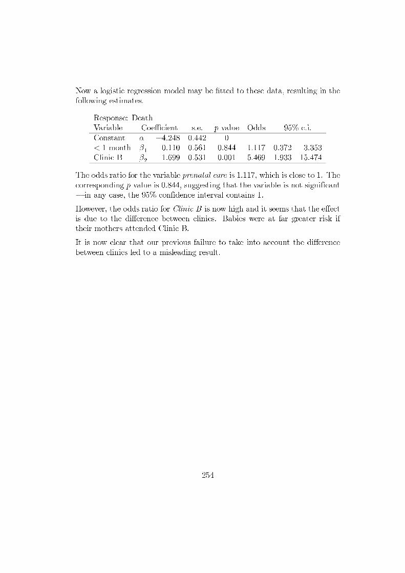
Now a logistic regression model may be fitted to these data, resulting in thefollowing estimates.

Response: DeathVariable Coefficient s.e. p-value Odds 95% c.i.Constant α −4.248 0.442 0< 1 month β1 0.110 0.561 0.844 1.117 0.372 3.353Clinic B β2 1.699 0.531 0.001 5.469 1.933 15.474

The odds ratio for the variable prenatal care is 1.117, which is close to 1. Thecorresponding p-value is 0.844, suggesting that the variable is not significant− in any case, the 95% confidence interval contains 1.

However, the odds ratio for Clinic B is now high and it seems that the effectis due to the difference between clinics. Babies were at far greater risk iftheir mothers attended Clinic B.

It is now clear that our previous failure to take into account the differencebetween clinics led to a misleading result.

254

13.5.1 Multiple risk factors

The power of logistic regression as a technique is well demonstrated by thefollowing example. The data were collected by Tuyns (1977) and come from acase-control study investigating risk factors for oesophagal cancer. Two riskfactors were considered.: average daily consumption of a) tobacco (g/day)and b) alcohol (g/day). The data were also classified into 10-year age groups.

Tobacco 0-9 Tobacco 10-19 Tobacco 20+Alcohol: 0-39 40-79 80+ 0-39 40-79 80+ 0-39 40-79 80+

Age Case 0 0 0 0 0 1 0 0 025-34 Cont 40 27 3 10 7 1 11 11 5Age Case 0 0 2 1 3 0 0 1 235-44 Cont 60 35 12 13 20 9 15 21 5Age Case 1 6 7 0 4 9 0 10 945-54 Cont 45 32 13 18 17 9 14 12 7Age Case 2 9 14 3 6 14 7 10 1455-64 Cont 47 31 14 19 15 8 11 28 5Age Case 5 17 9 4 3 5 2 5 565-74 Cont 43 17 8 10 7 9 7 4 1Age Case 1 2 3 2 1 2 1 1 075+ Cont 17 3 0 4 2 0 2 3 0

The risk factors are replaced by indicator variables before fitting the logisticregression model, giving a data array with 14 columns in all. One indicatorvariable is omitted from each of the three sets. The following was obtainedas a result of fitting the model after omitting the indicator variables corre-sponding to the lowest consumption levels of tobacco and alcohol and theage group 25-34 years.

255

Response: Oesophagal cancer

Variable Coefficient StErr p-value O.R.Constant α −6.269 1.037 0.000Tob 10− 19 β1 0.404 0.225 0.073 1.497Tob 20+ β2 0.861 0.223 0.000 2.367Alc 40− 79 β3 1.352 0.248 0.000 3.866Alc 80+ β4 2.486 0.261 0.000 12.011Age 35− 44 β5 1.550 1.070 0.148 4.713Age 45− 54 β6 3.205 1.028 0.002 24.647Age 55− 64 β7 3.701 1.023 0.000 40.501Age 65− 74 β8 4.181 1.031 0.000 65.436Age 75+ β9 4.350 1.080 0.000 77.470

The logistic model may be used to calculate an odds ratio for any two expo-sure groups. Such an odds ratio is

exp[∑

bj

(x(1)j − x(0)j

)]where the superscripts (1) and (0) designate the values of the predictorvariables in the two exposure groups.

It is easy to see why. Remember the way of modelling log-odds.

log

(p

1 − p

)= a+

∑bjxj,

so, for two groups designated by superscripts (1) and (0),

log

(p(1)

1− p(1)

)− log

(p(0)

1 − p(0)

)=∑

bj(x(1)j − x

(0)j

),

which is the log of the odds-ratio.

Suppose, for example, based on the output just obtained, you wish to com-pare the odds of disease for subjects consuming 10-19 grams/day of tobaccoand 40-79 grams/day of alcohol with those in the baseline group (0-9 gramsof tobacco and 0-39 grams of alcohol). The odds-ratio is

exp[∑

bj

(x(1)j − x

(0)j

)]256

and, with age accounted for, the only predictors contributing are x1 and x3,and the formula reduces to exp(b1 + b3), that is, exp(0.404 + 1.352) = 5.79.(This result may also be obtained by multiplying together the odds ratios1.497 and 3.866.)

The effect of two risk factors is thus obtained by adding their contributionsto the linear term in the model, which corresponds to multiplying their oddsratios, since the odds ratio is obtained by exponentiating the coefficient in thelinear term. The odds ratios for the various exposure groups (compared withthe baseline exposure group having the lowest tobacco and alcohol consump-tion) may thus be estimated using the model, and are given in the followingtable.

Alcohol Tobacco ConsumptionConsumption 0-9 g/day 10-19 g/day 20+ g/day0-39 g/day (1.0) 1.497 2.36740-79 g/day 3.866 5.787 9.15180+ g/day 12.011 17.980 28.430

As you have seen, the oesophagal cancer study provides a good illustrationof the fitting of a logistic regression model to data involving multiple riskfactors.

13.5.2 Continuous covariates

The models we have fitted up to now have all had explanatory variables whichare indicators. However, there is no reason why a continuous explanatoryvariable should not be fitted. In the previous example we had the variable agein six categories and used indicators. This, of course, loses the informationthat the age variable is ordered and it may be better to treat it as continuous.Furthermore, it will reduce the number of explanatory variables as age willneed only one rather than five.

Suppose we repeat the logistic regression for the oesophagal cancer data usinga single covariate for age, this being the middle of each age group (i.e. lowerend of age interval +5).

257

Response: Oesophagal cancer

Variable Coefficient StErr p-value O.R.Constant α −7.064 0.570 0.000Tob 10− 19 β1 0.416 0.224 0.063 1.516Tob 20+ β2 0.883 0.220 0.000 2.418Alc 40− 79 β3 1.404 0.248 0.000 4.071Alc 80+ β4 2.588 0.259 0.000 13.300Age β5 0.072 0.008 0.000 1.074

The standard errors have all been slightly reduced. The odds ratio for Agecan be interpreted as an odds ratio for a difference in age of one year. Theodds ratios for the various exposure groups are therefore as below.

Alcohol Tobacco ConsumptionConsumption 0-9 g/day 10-19 g/day 20+ g/day0-39 g/day (1.0) 1.516 2.41840-79 g/day 4.071 6.172 9.84480+ g/day 13.300 20.163 32.159

These have all come out a little higher than before.

258

13.6 Deviance

The estimates of β, and therefore of the probabilities

pi = g−1(xTi β

)were obtained by maximising the log-likelihood function l(p;y).

The goodness-of-fit of a model of this kind is assessed by looking at thelog-likelihood-ratio statistic

D = 2 [l(p̂s;y)− l(p̂;y)]

where p̂s is the vector of maximum likelihood estimates corresponding to thesaturated model and p̂ is the vector of maximum likelihood estimates for themodel of interest.This statistic is called the deviance.

For the saturatedmodel we take the pi’s to be the parameters to be estimated.Since Yi is binomially distributed,

∂l

∂pi=

yipi−ni − yi1 − pi

, giving pi =yini.

Then

D = 2n∑i=1

[yi log

(yinip̂i

)+ (ni − yi) log

(ni − yini − nip̂i

)].

D has the familiar form

2n∑i=1

ni log

(ninπ̂i

)

which we met when we first looked at goodness-of-fit of distributions todata, where the ni here represent cell frequencies. We are tempted to think,therefore, thatD has asymptotically a χ2-distribution. There are no nuisanceparameters and so goodness-of-fit ought to be assessed directly using theapproximation

DD→ χ2(n− p),

where p is the number of β parameters estimated.

DIRE WARNING! Alas this is not true for binary data and, contrary toanything you may read in the literature, D may not be used for assessing

259

goodness-of-fit. For a detailed discussion of the inadequacy of this statistic,see Generalized Linear Models by McCullagh and Nelder, page 118.

However, the deviance is extremely useful for comparing two nested models.If we wish to test whether the addition of a further covariate significantlyimproves the fit, the reduction in deviance is distributed as χ2(1) indepen-

dently of β̂. In order for this to be the case, D itself does not need to havean approximate χ2-distribution; neither need it be independent of β̂. Theχ2 approximation is quite accurate for differences in deviances, even thoughinaccurate for the deviances themselves.

Let us see how this works in practice by doing an example.

Example Depression in adolescents

The data come from a study by Maag and Behrens (1989) of seriously emo-tionally disturbed (SED) and learning disabled (LD) adolescents. The dataare given as a four-way contingency table.

DepressionAge Label Sex Low High

LD Male 79 1812-14 Female 34 14

SED Male 14 5Female 5 8

LD Male 63 1015-16 Female 26 11

SED Male 32 3Female 15 7

LD Male 36 1317-18 Female 16 1

SED Male 36 5Female 12 2

There is no chance of a purely main effects model fitting these data, so wemight as well put in interactions from the start. For example, we know thatgirls and boys mature at different rates, so it makes sense to have a Sex-Age

260

interaction. Suppose we set up the data with the following variables:

1. Depressed Number with high depression in group2. Total Total number in group4. Female Female = 1, Male = 06. SED SED = 1, LD = 07. 12-148. 15-16 Age indicator variables9. 17-18

Variables representing interactions are created by multiplying together corre-sponding entries of the individual variables. That is, if the variable Female isrepresented by a vector of indicator variables {fi} and if SED is representedby {si}, then the vector representing the interaction of the variables is {fisi}.

Using learning disabled males aged 12-14 as the reference group, the outputfrom fitting the full model is given below.

Variable Coefficient StErr p-value O.R.Constant α −1.473 0.254 0.000Female β1 0.576 0.385 0.134 1.779SED β2 0.417 0.506 0.409 1.518Age 15-16 β3 −0.320 0.400 0.424 0.726Age 17-18 β4 0.399 0.404 0.323 1.491Fem/SED β5 0.980 0.577 0.089 2.664Fem/15-16 β6 0.301 0.556 0.588 1.351Fem/17-18 β7 −1.826 0.773 0.018 0.161SED/15-16 β8 −1.157 0.637 0.069 0.314SED/17-18 β9 −1.206 0.689 0.080 0.299

The deviance is 0.644.

Now we shall try dropping variables, in turn according to the p-value of thecoefficient.

See what happens to the deviance each time we drop a variable.

Dropped None 6 3,6 2,3,6 2,3,4,6 2,3,4,6,9Deviance 0.644 0.938 1.298 2.200 3.838 5.172

The largest difference is 1.638. Tested as χ2(1) the p-value is 0.201, so thatno significant difference is seen each time a variable is dropped. Dropping

261

the 5 variables has only changed the deviance by 4.528.

However, dropping one more variable does make a difference. The variablewhich causes the smallest change when dropped is variable 8, which resultsin a deviance of 10.437 when the reduced model is fitted. The difference is5.265. Tested as χ2(1) the p-value is 0.022.

You can play around with other models and interactions, but eventually youwill come down to the following model.

Variable Coefficient StErr p-value O.R.Constant α −1.489 0.152 0.000Female β1 0.621 0.279 0.026 1.860Fem/SED β5 1.189 0.482 0.014 3.283Fem/17-18 β7 −2.042 0.690 0.003 0.130SED/15-16 β8 −1.011 0.475 0.033 0.364

How should you interpret these results?

Clearly Age and SED do not, of themselves, have a significant effect on therisk of severe depression, but there is a significant difference between theeffect of serious emotional disturbance and learning disability in certain age

and sex groups. Whilst females from the serious emotionally disturbed groupare at very much greater risk (OR = 3.28), the reverse is true for femalesaged 17-18 (OR = 0.13) and for both sexes aged 15-16 (OR = 0.36).

We conclude that females with learning disability from the 12-14 age groupand males from the 17-18 age group are more likely to experience severedepressive symptomatology.

A cricketing controversyIn December 1991 the Indian cricket team was comprehensively defeated byAustralia in the first two test matches at Brisbane and Melbourne. Theformer captain of India, Sunil Gavaskar, subsequently wrote a newspapercolumn in which he claimed that Australian umpires were biased in favour ofthe home team, particularly with regard to controversial LBW (leg-before-wicket) decisions. A major media row followed and on January 5, 1992 theSydney Sun-Herald newspaper entered the lists by producing figures for LBWdecisions against top-order batsmen in Australian tests from 1977 onwards.

262

The figures published in the Sun-HeraldJanuary 5, 1992

LBW decisions against top-order batsmenin Australian tests from 1977 onwards

Australia OtherLBW dismissals 95 121Number of innings 855 874

Gavaskar’s response to the Sun-Herald was “the figures speak for them-selves”. Can a statistician shed any light upon the issue?

Australia (x = 0) Other (x = 1)LBW dismissals (y = 1) 95 121Other dismissals (y = 0) 760 753

Fitting a logistic regression,

Coefficient Odds Ratioα −2.079β 0.251 1.285

Gavaskar’s claim looks a bit shaky.

But the plot thickens. As the row with Gavaskar developed, the Sun-Heraldsubsequently went on to give a more complete listing of the LBW decisionsin test matches held in Australia.

263

No. of No. ofTest Series Australia Innings Other Inningsvs India 1977-78 7 60 3 54vs England 1978-79 5 72 18 68vs Pakistan 1978-79 2 22 1 24vs England 1979-80 3 34 6 36vs W. Indies 1980-81 6 36 3 31vs N. Zealand 1980-81 2 30 5 36vs India 1980-81 1 30 6 36vs Pakistan 1981-82 3 32 5 30vs W. Indies 1981-82 4 36 4 56vs England 1982-83 6 56 3 60vs Pakistan 1983-84 6 38 5 53vs W. Indies 1984-85 6 54 5 52vs N. Zealand 1985-86 4 36 3 30vs India 1985-86 3 32 1 22vs England 1986-87 7 59 8 51vs N. Zealand 1987-88 6 27 4 36vs England 1987-88 0 10 0 6vs Sri lanka 1987-88 1 6 4 12vs W. Indies 1988-89 6 59 8 57vs N. Zealand 1989-90 1 6 3 12vs Sri lanka 1989-90 3 24 4 18vs Pakistan 1989-90 6 28 7 30vs England 1990-91 6 50 13 60vs India 1991-92 1 18 2 24

If we fit a logistic model with the variables shown below,

i xi = 1 xi = 01 England Other2 India Other3 Pakistan Other4 New Zealand Other5 West Indies Other6 Sri Lanka Other

we obtain the following.

264

Coefficient Odds RatioConstant α −2.079England β1 0.716 2.046India β2 −0.256 0.774Pakistan β3 0.191 1.211NZ β4 0.192 1.212WI β5 −0.095 0.909SL β6 1.068 2.910

Conclusion

� There is no justification for Gavaskar’s claim, unless he is making it onbehalf of Sri Lanka.

Note that the Australians have not played a large number of gamesagainst Sri lanka. However, it can be shown that the odds ratio issignificantly different from 1.

� But what about decisions against England. With a sample of size 47 itis hardly surprising that the odds ratio can be shown to be significantlydifferent from 1. We conclude that Pommies have double the odds ofbeing given out LBW.

Psychological Momentum

There is a widespread belief in many sports that “success breeds success andfailure breeds failure.”

To put it another way, does winning one trial improve a player’s chances ofwinning the next?

Sports commentators refer to this as momentum or psychological momentum

and nowhere is the expression used more than in the sport of tennis.

So let us ask the question: “In a best of five sets tennis match, does the prob-ability of winning change as the match progresses and is there any evidencefor the existence of psychological momentum?”

265

The data and the model

The data comprise 501 matches between top ranking players which cover1847 sets. All matches were played in the 1987 and 1988 Wimbledon andU.S. Open Tournaments.

The model is an odds model which assesses the odds O that a player rankedr in the World Rankings beats, in the first set, a player ranked s as

O =(sr

)α

or, equivalently

log(Odds) = α log(sr

)where α is to be determined from the data.

Psychological momentum

A possible model for this is to define Oij to be the odds of winning the nextset when the score is (i, j) in sets and use the idea that winning a set increasesthe odds of winning the next set by a factor of k.

In such a model,Oij = ki−jO00

where O00 are the odds in the first set.

O

kO

k−1O

O

k2O

k−2O

Odds

win

lose

win

lose

win

lose

266

Comparing the models

Model 1.log(Odds) = α log

(sr

)Fitting the model to the data we find α = 0.510.

Model 2.log(Odds) = α log

(sr

)+ (i− j) log k

We find α = 0.441 and k = 1.48.

Results for the higher ranked player of 501 matches in the1987

and 1988 Wimbledon and U.S. Open Tournaments

Result Observed Model 1 Model 23− 0 191 158.3 193.73− 1 104 132.8 112.33− 2 57 87.2 58.82− 3 36 52.7 36.71− 3 54 44.6 49.10− 3 59 25.5 50.5

The expected values in this table are given using the estimates obtainedabove.

Conclusion

The fit of Model 2 is very good indeed. This would seem to be compellingevidence for the existence of psychological momentum.

267