26 February 2006Eric Rasmusen, Erasmuse@indiana.edu, Http://www.rasmusen.org.

13 Auctions

13.1 Values Private and Common, Continuous and Discrete

Bargaining and auctions are two extremes in the many ways to sell goods, as Bulow & Klem-perer (1996) explain. In typical bargaining, one buyer faces one seller and they make offersand counteroffers free from the formal rules we impose in theoretical modelling (though asin Bulow and Klemperer, it is worth considering what happens if the bargaining does haverules to which the players commit). In typical auctions, many bidders face one seller andmake offers according to formal rules as rigid as those of the theorist. Bargaining is slowbut flexible; auctions are fast but rigid.

Bargaining models generate different results with different assumptions, but since itis usually hard to match the assumptions with particular real situations, the practicalimplications come from the simplest models– ideas such as the importance of avoidingmisunderstanding, determining and then concealing one’s own reservation price, bluffing,and manipulating the timing of offers.

Auction models, on the other hand, may also generate different results with differentassumptions but it is easier to match the assumptions with particular real situations, oreven to create a real situation to match the model. That is because auctions vary notonly in the underlying preferences of the players, as in bargaining, but in the specific rulesused to play the game, and those rules are chosen by one of the players, usually with legalcommitment to them. Thus, auction theory lends itself to what Alvin Roth (2002) calls“the economist as engineer”: the use of technical economic theory to design institutionsfor specific situations. As with other engineering, the result may not be of general interest,but tailoring the model to the situation is both tricky and valuable, requiring the samekind of talent and care as developing the general theory.

Because auctions are stylized markets with well-defined rules, modelling them withgame theory is particularly appropriate. Moreover, several of the motivations behind auc-tions are similar to the motivations behind the asymmetric information contracts of Part IIof this book. Besides the mundane reasons such as speed of sale that make auctions impor-tant, auctions are useful for a variety of informational purposes. Often bidders know morethan the seller about the value of what is being sold, and the seller, not wanting to suggesta price first, uses an auction as a way to extract information. Art auctions are a goodexample, because the value of a painting depends on the bidder’s tastes, which are knownonly to himself. Efficient allocation of resources is a goal different from profit maximization,but auctions are useful for that too. A good example is told in Boyes and Happel’s 2001article, “Auctions as an Allocation Mechanism in Academia: The Case of Faculty Offices.”At their business school, the economics department used an auction to allocate new offices,whereas the management department used seniority, the statistics department used dice,

404

and the finance department posted a first-come first-serve sign-up sheet without warning.The auction has the best chance of coming up with an immediate efficient allocation. (Whydo I say “immediate”? Why would the long-run probably stay the same?)

Auctions are also useful for agency reasons, because they hinder dishonest dealing.If the mayor were free to offer a price for building the new city hall and accept the firstcontractor who showed up, the lucky contractor would probably be the one who made thebiggest political contribution. If the contract is put up for auction, cheating the public ismore costly, and the difficulty of rigging the bids may outweigh the political gain.

We will spend most of this chapter on the effectiveness of different kinds of auctionrules in extracting surplus from bidders, which will require finding the strategies with whichbidders respond to the rules. Section 13.1 classifies auctions based on the relationshipsbetween different bidders’ estimates of the value of what is being auctioned. Section 13.2,a necessarily very long section, explains the possible auction rules and the bidding strategiesoptimal for each rule. Section 13.3 compares the outcomes under the various rules, provingthe Revenue Equivalence Theorem and showing how it becomes invalid if bidders are riskaverse. Section 13.4 shows how to choose an optimal reserve price using the similaritybetween optimal auctions and monopoly pricing. Section 13.5 analyzes common-valueauctions, which can lead bidders into “the winner’s curse” if they are not careful. Section13.6 discusses asymmetric equilibria (The Wallet Game) and information affiliation.

Private-Value and Common-Value Auctions

Auctions differ enough for an intricate classification to be useful. One way to classifyauctions is based on differences in the values bidders put on what is being auctioned. Wewill call the dollar value of the utility that bidder i receives from an object its value tohim, vi, and we will denote his estimate of the value by vi.

In a private-value auction, a bidder can learn nothing about his value from knowingthe values of the other bidders. An example is the sale of antique chairs to people whowill not resell them. Usually a bidder’s value equals his value estimate in private-valueauction models. If an auction is to be private- value, it cannot be followed by costlessresale of the object. If there were resale, a bidder’s value would depend on the price atwhich he could resell, which would depend on the other bidders’ values. What is specialabout a private- value auction is that a bidder cannot extract any information about hisown value from the value estimates of the other bidders. Knowing all the other values inadvance would not change his estimate. It might well change his bidding strategy, however,so we distinguish between the independent private-value auction, in which knowinghis own value tells him nothing about other bidders’ values, and other situations such asthe affiliated private-value auction (affiliation being a concept which will be explainedlater) in which he might be able to use knowledge of his own value to deduce somethingabout other players’ values.

In a pure common-value auction, the bidders have identical values, but each bidderforms his own estimate on the basis of his own private information. An example is biddingfor U. S. Treasury bills. A bidder’s estimate would change if he could sneak a look at theother bidders’ estimates, because they are all trying to estimate the same true value.

405

The values in most real-world auctions are a combination of private value and commonvalue, because the value estimates of the different bidders are positively correlated but notidentical. As always in modelling, we trade off descriptive accuracy against simplicity. Itis common for economists to speak of mixed auctions as “common-value” auctions, sincetheir properties are closer to those of common-value auctions. Krishna (2002) has used theterm interdependent value for the mixed case.

The private-value/common-value dichotomy is about what a bidder knows about hisown value, but a separate dimension of auctions is what a bidder knows about other bidders’values. One possibility is that the values are common knowledge. This makes optimalbidding simple. In a private-value auction, the highest- valuing bidder can bid just above thesecond-highest value. In a common-value auction, the bidders will take into account eachothers’ information and their value estimates will instantly converge to a single commonestimate, the best one given all available information. In either case, bidders don’t haveto worry about cleverly deducing each others’ information by observing how the biddingproceeds.

It would be odd, however, to observe an auction in the real world in which the sellerknew the value estimates. In that case, the seller shouldn’t be using an auction. He shouldjust charge a price equal to the highest value estimate, a price he knows will be acceptedby one of the bidders.

More commonly, only the bidder himself knows his value, not other bidders or theseller. Most simply, the estimated values are statistically independent, the independentprivate- value case that we will be analyzing for the first half of this chapter. If theestimates are independent, then a bidder’s only source of information about his value is hisprivate information and his only source of information about other bidders’ value estimatesis what he observes of their bidding. If the value estimates are not independent, a biddercan use his private information to help estimate other bidders’ values (and thus how theywill bid), and if he does not know his own value perfectly he can use observations of theirvalue estimates to improve his estimate of his own value— which takes us to the commonvalue case.

Lack of statistical independence can be present even in private-value auctions, however.Smith might know his own value perfectly, and so would not be able to learn anything aboutit by learning Jones’s value. That is what makes the auction a private-value auction. Butif the values are not independent— if, say they are positively correlated— then if Smithknows that his own value is unusually high he could predict that Jones’s value was also high.This would affect Smith’s bidding strategy, even though it would not affect the maximumhe would be willing to pay for the object being sold. I will not be analyzing private-valueauctions with correlated values here, but as explained in Riley (1989) the difference canbe important. Although bidding in the ascending and second-price auction rules that wewill soon discuss is unchanged when values are correlated, bidding becomes lower in thedescending and first-price auctions. In contrast, we will see that bidding in a common-valueauction is generally more cautious than in a private-value auction even in ascending andsecond-price auctions.

To look at these various auction rules, we will use the following two games, which I

406

have set up using the language of mechanism design since choosing auction rules fits wellinto that paradigm. The Ten-Sixteen Auction will be our running example for when valuesare discrete (v = 10 or v = 16), and the Continuous-Value Auction will be our example forwhen they are on a continuum (v ∼ f(v) on [v, v]).

The Ten-Sixteen Auction

Players: One seller and two bidders.

Order of Play:0. Nature chooses Bidder i’s value for the object to be either vi = 10 or vi = 16, with equalprobability. (The seller’s value is zero.)1. The seller chooses a mechanism [G(vi, v−i)vi− t(vi, v−i)] that takes payments t and givesthe object with probability G to player i (including the seller) if he announces that hisvalue is vi and the other players announce v−i. He also chooses the procedure in whichbidders select vi (sequentially, simultaneously, etc.).2. Each bidder simultaneously chooses to participate in the auction or to stay out.3. The bidders and the seller choose v according to the mechanism procedure.4. The object is allocated and transfers are paid according to the mechanism.

Payoffs:The seller’s payoff is

πs =n∑

i=1

t(vi, v−i) (1)

Bidder i’s payoff is zero if he does not participate, and otherwise is

πi(vi) = G(vi, v−i)vi − t(vi, v−i) (2)

To get around the open-set problem, we will assume for any auction rule that tiesare broken in favor of whoever has the highest value, or randomly if the values are equal.Otherwise, if, for example, we said that ties simply split the probability of winning, thenif v1 = 10 and v2 = 16 and this were known to both bidders, it would not be even a weakequilibrium to have them bid p1 = 10 and p2 = 10, because Bidder 2 would deviate toa slightly higher bid– but the smallest bid strictly greater than 10 does not exist if bidincrements can be infinitesimal.

The second game will be our example for when values lie on a continuum.

The Continuous-Value Auction

Players: One seller and two bidders.

Order of Play:0. Nature chooses Bidder i’s value for the object, vi, using the strictly positive, atomless

407

density f(v) on the interval [v, v].1. The seller chooses a mechanism [G(vi, v−i)vi− t(vi, v−i)] that takes payments t and givesthe object with probability G to player i (including the seller) if he announces that hisvalue is vi and the other players announce v−i. He also chooses the procedure in whichbidders select vi (sequentially, simultaneously, etc.).2. Each bidder simultaneously chooses to participate in the auction or to stay out.3. The bidders and the seller choose v according to the mechanism procedure.4. The object is allocated and transfers are paid according to the mechanism, if it wasaccepted by all bidders.

Payoffs:The seller’s payoff is

πs =n∑

i=1

t(vi, v−i) (3)

Bidder i’s payoff is zero if he does not participate, and otherwise is

πi(vi) = G(vi, v−i)vi − t(vi, v−i) (4)

Many possible auction procedures fit the mechanism paradigm, even ones that arenever used in practice. The mechanism could allocate the good with 70% probability tothe high bidder and with 30% probability to the lowest bidder, for example; or each biddercould be made to pay the amount he bids, even if he loses; or t could include an entry fee;or there could be a “reserve price,” a minimum bid for which the seller will surrender thegood. In this analysis, the seller will choose a direct mechanism that satisfies a participationconstraint for each bidder type vi (Bidder i will join the auction, so, for example, the entryfee is not too large), and an incentive compatibility constraint (the bidder will truthfullyreveal his type; vi = vi).

13.2 Optimal Strategies under Different Rules in Private-Value Auctions

Auctions have the same bewildering variety of rules as poker does. We will look at fivedifferent auction rules, using the private-value setting since it is simplest. In teaching thismaterial, I ask each student to pick a value between 80 and 100, after which we conductthe various kinds of auctions. I advise the reader to try this. Pick two values and try outsample strategy profiles for the different auctions as they are described. Even though thevalues are private, it will immediately become clear that the best-response bids still dependon the strategies the bidder thinks other bidders have adopted.

The five auction rules we will consider (with common synonyms for them) are :

1 Ascending (English, open-cry, open-exit);2 First-Price (first-price sealed-bid);3 Second-Price (second-price sealed-bid, Vickrey);4 Descending (Dutch)5 All-Pay

408

Ascending (English, open-cry, open-exit)

RulesEach bidder is free to revise his bid upwards. When no bidder wishes to revise his bidfurther, the highest bidder wins the object and pays his bid.

StrategiesA bidder’s strategy is his series of bids as a function of (1) his value, (2) his prior estimateof other bidders’ values, and (3) the past bids of all the bidders. His bid can therefore beupdated as his information set changes.

PayoffsThe winner’s payoff is his value minus his highest bid (t = p for him and t = 0 for everyoneelse). The losers’ payoffs are zero.

DiscussionA bidder’s dominant strategy in a private-value ascending auction is to stay in the biddinguntil bidding higher would require him to exceed his value and then to stop. This is optimalbecause he always wants to buy the object if the price is less than its value to him, but hewants to pay the lowest price possible. All bidding ends when the price reaches the second-highest value of any bidder present at the auction. The optimal strategy is independentof risk neutrality if bidders know their own values with certainty rather than having toestimate them, although risk-averse bidders who must estimate their values should bemore conservative in bidding.

The optimal private-value strategy is simple enough that details of the ascendingauction usually do not make much difference, but there are a number of possibilities.

(1) The bidders offer new prices using pre-specified increments such as dollars or thousandsof dollars.(2) The open-exit auction, in which the price rises continuously and bidders show theirwillingness to pay the price by not dropping out, where a bidder’s dropping out is publiclyannounced to the other bidders.(3) The silent-exit auction (my neologism), in which the price rises continuously and bid-ders show their willingness to pay the price by not dropping out, but a bidder’s droppingout is not known to the other bidders.(4) The Ebay auction, in which a bidder submits his “bid ceiling,” the maximum pricehe is willing to pay. During the course of the auction the seller uses the bid ceilings to raisethe current winning bid only as high as necessary, and the winner is the player whose bidis highest at a prespecified ending time.(5) The Amazon auction, in which a bidder submits his bid ceiling. During the courseof the auction the seller uses the bid ceilings to raise the current winning bid only ashigh as necessary, and the winner is the player whose bid is highest at a prespecified end-ing time or ten minutes after the last increase in the current winning bid, whichever is later.

409

The precise method can be quite important in common-value auctions, where knowingwhat other players are doing alters a bidder’s own value estimate. If the auction is open-exit, for example, a bidder who observed that most of the other bidders dropped out ata low price would probably revise his own value estimate downwards, something he wouldnot know to do in a silent-exit auction.

The ascending auction can be seen as a mechanism in which each bidder announceshis value (which becomes his bid), the object is awarded to whoever announces the highestvalue (that is, bids highest), and he pays the second-highest announced value (the second-highest bid). In the Continuous-Value Auction, denote the highest announced value byv(1), the second-highest by v(2), and so forth. the highest bidder gets the object withprobability G(v(1), v−1) = 1 at price t(v(1), v−1) = v(2), and for i 6= 1, G(v(i), v−i) = 0 andt(v(1), v−1) = 0. This is incentive compatible, since a player’s value announcement onlymatters if his value is highest, and he then wants to win if and only if the price is less thanor equal to his value. It satisfies the participation constraint because his lowest possiblepayoff following that strategy is zero, and his payoff is higher if he wins and v(1) > v(2).

Since each bidder’s expected payoff is strictly positive, the optimal mechanism for theseller would be more complicated. As we will discuss later, it would include a reserve pricep∗ below which the object would remain unsold, changing the first part of the mechanismto G(v(1), v−1) = 1 and t(v(1), v−1) = Max{v(2), p

∗} if v(1) ≥ p∗ but G(v(1), v−1) = 0 ifv(1) < p∗. We have seen in Chapter 10 that optimal mechanisms are not always efficient,and this is an example: the object will go unsold if v(1) < p∗.

In the Ten-Sixteen Auction, the seller’s value is vs = 0, and each of two bidders’ privatevalues v1 and v2 is either 10 or 16 with equal probability, known only to the bidder himself.A bidder’s optimal strategy in the ascending auction would be to set his bid or bid ceilingto p(v = 10) = 10 and p(v = 16) = 16. His expected payoff would be

π(v = 10) = 0

π(v = 16) = 0.5(16− 10) + 0.5(16− 16) = 3(5)

The expected price, the payoff to the seller, is

πs = 0.52(10) + 0.52(16) + 2(0.5)2(10) = 2.5 + 4 + 5 = 11.5 (6)

First-Price (first-price sealed-bid)

RulesEach bidder submits one bid, in ignorance of the other bids. The highest bidder pays hisbid and wins the object.

StrategiesA bidder’s strategy is his bid as a function of his value.

PayoffsThe winner’s payoff is his value minus his bid. The losers’ payoffs are zero.

410

DiscussionIn the first-price auction what the winning bidder wants to do is to have submitted a sealedbid just enough higher than the second-highest bid to win. If all the bidders’ values arecommon knowledge and he can predict the second- highest bid perfectly, this is a simpleproblem. If the values are private information, then he has to guess at the second-highestbid, however, and take a gamble. His tradeoff is between bidding high–thus winning moreoften–and bidding low–thus benefiting more if the bid wins. His optimal strategy dependson his degree of risk aversion and beliefs about the other bidders, so the equilibrium is lessrobust to mistakes in the assumptions of the model than the equilibria of ascending andsecond-price auctions. As we will see later, however, there are good reasons why sellers sooften choose to use first-price auctions.

The First-Price Auction with a Continuous Distribution of Values

Suppose Nature independently assigns values to n risk-neutral bidders using the con-tinuous density f(v) > 0 (with cumulative probability F (v)) on the support [0, v].

A bidder’s payoff as a function of his value v and his bid function p(v) is, lettingG(p(v)) denote the probability of winning with a particular p(v):

π(v, p(v)) = G(p(v))[v − p(v)]. (7)

Let us first prove a lemma.

Lemma: If player’s equilibrium bid function is differentiable, it is strictly increasing in hisvalue: p′(v) > 0.

Proof: The first-order condition from payoff (7) is

dπ(v)

dp= G′(v − p)−G = 0. (8)

The optimum is an interior solution because at pi = 0 the payoff is increasing and if pi

becomes large enough, π is negative. Thus, d2π(vi)

dp2i≤ 0 at the optimum. Using the implicit

function theorem and the fact that d2π(vi)dpidvi

= G′ ≥ 0 because a higher bid does not yield a

lower probability of winning, we can conclude that dpi

dvi≥ 0, at least if the bid function is

differentiable. But it cannot be that dpi

dvi= 0, because then there would be values v1 and v2

such that p1 = p2 = p and then

dπ(v1)

dp1

= G′(p)(v1 − p)−G(p) = 0 =dπ(v2)

dp2

= G′(p)(v2 − p)−G(p), (9)

which cannot be true. So the bidder bids more if his value is higher. Q.E.D.

Now let us try to find an equilibrium bid function. From equation (7), it is

p(v) = v − π(v, p(v))

G(p(v)). (10)

That is not very useful in itself, since it has p(v) on both sides. We need to find ways torewrite π and G in terms of just v.

411

First, tackle G(p(v)). Monotonicity of the bid function (from Lemma 1) implies thatthe bidder with the greatest v will bid highest and win. Thus, the probability G(p(v)) thata bidder with price pi will win is the probability that vi is the highest value of all n bidders.The probability that a bidder’s value v is the highest is F (v)n−1, the probability that eachof the other (n− 1) bidders has a value less than v. Thus,

G(p(v)) = F (v)n−1. (11)

Next think about π(v, p(v)). The Envelope Theorem says that if π(v, p(v)) is the valueof a function maximized by choice of p(v) then its total derivative with respect to v equalsits partial derivative, because ∂π

∂p= 0:

dπ(v,p(v))dv

= ∂π(v,p(v))∂p

∂p∂v

+ ∂π(v,p(v))∂v

= ∂π(v,p(v))∂v

. (12)

We can apply the Envelope Theorem to equation (7) to see how π changes with v assumingp(v) is chosen optimally, which is appropriate because we are characterizing not just anybid function, but the optimal bid function. Thus,

dπ(v, p(v))

dv= G(p(v)). (13)

Substituting from equation (11) gives us π’s derivative, if not π, as a function of v:

dπ(v, p(v))

dv= F (v)n−1. (14)

To get π(v, p(v)) from its derivative, (14), integrate over all possible values from zero to vand include the a base value of π(0) as the constant of integration:

π(v, p(v)) = π(0) +

∫ v

0

F (x)n−1dx =∫ v

0F (x)n−1dx. (15)

The last step is true because a bidder with v = 0 will never bid a positive amount and sowill have a payoff of π(0, p(0)) = 0.

412

We can now return to the bid function in equation (10) and substitute for G(p(v)) andπ(v, p(v)) from equations (11) (15):

p(v) = v −∫ v

0F (x)n−1dx

F (v)n−1. (16)

Suppose F (v) = v/v, the uniform distribution. Then (16) becomes

p(v) = v −∫ v

0

(xv

)n−1dx(

vv

)n−1

= v −

∣∣∣∣vx=0

(1v

)n−1 ( 1n

)xn(

vv

)n−1

= v −(

1v

)n−1 ( 1n

)vn − 0(

vv

)n−1

= v − vn

=(

n−1n

)v.

(17)

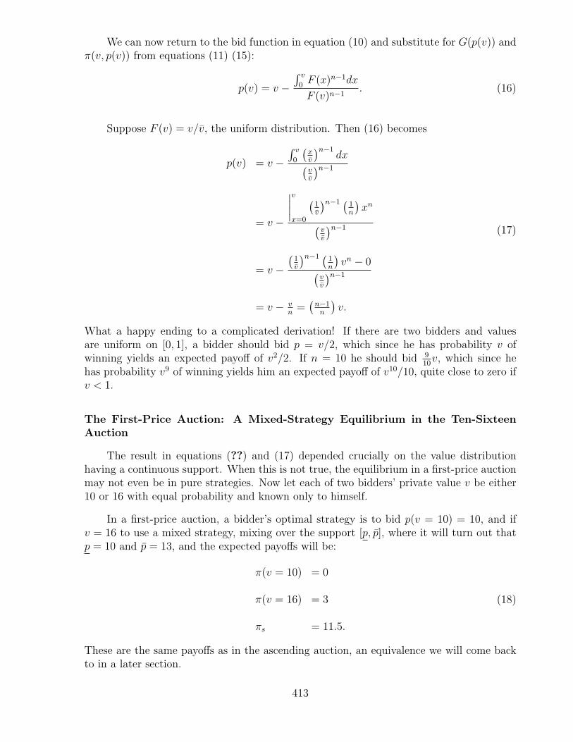
What a happy ending to a complicated derivation! If there are two bidders and valuesare uniform on [0, 1], a bidder should bid p = v/2, which since he has probability v ofwinning yields an expected payoff of v2/2. If n = 10 he should bid 9

10v, which since he

has probability v9 of winning yields him an expected payoff of v10/10, quite close to zero ifv < 1.

The First-Price Auction: A Mixed-Strategy Equilibrium in the Ten-SixteenAuction

The result in equations (??) and (17) depended crucially on the value distributionhaving a continuous support. When this is not true, the equilibrium in a first-price auctionmay not even be in pure strategies. Now let each of two bidders’ private value v be either10 or 16 with equal probability and known only to himself.

In a first-price auction, a bidder’s optimal strategy is to bid p(v = 10) = 10, and ifv = 16 to use a mixed strategy, mixing over the support [p, p], where it will turn out thatp = 10 and p = 13, and the expected payoffs will be:

π(v = 10) = 0

π(v = 16) = 3

πs = 11.5.

(18)

These are the same payoffs as in the ascending auction, an equivalence we will come backto in a later section.

413

This will serve as an illustration of how to find an equilibrium mixed strategy whenbidders mix over a continuum of pure strategies rather than just between two. The firststep is to see why the equilibrium cannot be in pure strategies (though some portions of theequilibrium strategy can be pure, e.g. if v = 10, a bidder will bid p = 10 with probabilityone).

First, there is no equilibrium in pure strategies, either symmetric or asymmetric. Inany equilibrium, p(v = 10) = 10, because if either bidder used the bid p < 10, it wouldcause the other player to deviate to (p + ε), and a bid above 10 exceeds the object’s value.

If v = 16, however, a player will randomize his bid, as I will now show. Supposethe two bidders are using the pure strategies p1(v1 = 16) = z1 and p2(v2 = 16) = z2.The values of z1 and z2 would lie in (10, 16] because a bid of exactly 10 would lose to thepositive-probability bid of p(v = 10) = 10 given our tie-breaking assumption and a bidover 16 would exceed the object’s value. yield a negative payoff. Either z1 = z2, or z1 6= z2.If z1 = z2, then each bidder has incentive to deviate to (z1 − ε) and win with probabilityone instead of tying. If z1 < z2, then Bidder 2 will deviate to bid (z1 + ε). If he does that,however, Bidder 1 would deviate to bid (z1 + 2ε), so he could win with probability one attrivially higher cost. The same holds true if z2 < z1. Thus, there is no equilibrium in purestrategies.

The second step is to figure out what pure strategies will be mixed between by abidder with v = 16. It turns out that they form the interval [10, 13]. As just explained,the bid p(v = 16) will be no less than 10 (so the bidder can win if his rival’s value is 10)and no greater than 16 (which would always win, but unprofitably). The pure strategy of(p = 10)|(v = 16) will win with probability of at least 0.50 (when the other bidder happensto have v = 10, given our tie-breaking rule), yielding a payoff of 0.50(16 − 10) = 3. Thisrules out bids in (13, 16], since even if they always win, their payoff is less than 3. Thus,the upper bound p must be no greater than 13.

The lower bound p must be exactly 10. If it were at (10 + ε) then a bid of (10 − 2ε)would have an equal certainty of winning the auction, but would have ε higher payoff.Thus, p = 10.

The upper bound p must be exactly 13. If it were any less, then the other playerwould respond by using the pure strategy of (p + ε), which would win with probabilityone and yield a payoff of greater than the payoff of 3 (= 0.5(16 − 10)) from p = 10. In amixed-strategy equilibrium, though, the payoff from any of the strategies mixed betweenmust be equal. Thus, p cannot be less than 13.

We are not quite done looking at the strategies mixed between. When a player mixesover a continuum, the modeller must be careful to check for (a) atoms (some particularpoint which has positive probability, not just positive density), and (b) gaps (intervalswithin the mixing range with zero probability of bids). Are there any atoms or gaps withinthe interval [10,13]? No, it turns out.

414

(a) Bidder 2’s mixing density does not have an atom at any point a in [10, 13]– no point ahas positive probability, as opposed to positive density. An example of such an atom wouldbe if the mixing distribution were the density m(p) = 1/6 over the interval [10, 13] plusan atom of probability 1/2 at p = 13, so the cumulative probability would be M(p) = p/6over [10, 13) and M(13) = 1. Using M(p), a point such as 11 would have zero probabilityeven though the interval, say, of [10.5, 12.5] would have probability 2/6.

If there were an atom at a, Bidder 1 would respond by putting positive probabilityon (a + ε) and zero probability on a. But then Bidder 2 would respond by putting zeroprobability on a and shifting that probability to (a + 2ε).

(b) Bidder 2’s mixing density does not have a gap [g, h] anywhere with g > 10 and h < 13.If it did, then Bidder 1’s payoff from bidding g and h would be

π1(g) = Prob(p2 < g)v1 − g (19)

andπ1(h) = Prob(p2 < h)v1 − h = Prob(p2 < g)v1 − h, (20)

where the second equality in π1(h) is true because there is zero probability that p2 isbetween g and h. Bidder 1 will put zero probability on p1 = h, since its payoff is lower thanthe payoff from p1 = g and will put zero probability on slightly larger values of p1 too, sinceby continuity their payoffs will also be less than the payoff from p1 = g. This creates a gap[h, h∗] in which p1 = 0. But then Bidder 2 will want to put zero probability on p2 = h∗ andslightly higher values, by the same reasoning, which means that our original hypothesis ofonly a gap [g, h] is false.

Thus, we can conclude that the mixing density m(p) is positive over the entire interval[10, 13], with no atoms. What will it look like? Let us confine ourselves to looking for asymmetric equilibrium, in which both bidders use the same function m(p). We know theexpected payoff from any bid p in the support must equal the payoff from p = 10 or p = 13,which is 3. Therefore, since if our player has value v = 16 there is probability 0.5 of winningbecause the other player has v = 10 and probability 0.5M(p) of winning because the otherplayer has v = 16 too but bid less than p, the payoff is

0.5(16− p) + 0.5M(p)(16− p) = 3. (21)

This implies that (16− p) + M(p)(16− p) = 6, so

M(p) =6

16− p− 1, (22)

which has the density

m(p) =6

(16− p)2(23)

on the support [10, 13], rising from m(10) = 16

to m(13) = 46.

Since each bidder type has the same expected payoff in this first-price auction as in theascending auction, and the object is sold with probability one, it must be that the seller’spayoff is the same, too, equal to 11.5, as we found in equation (6).

415

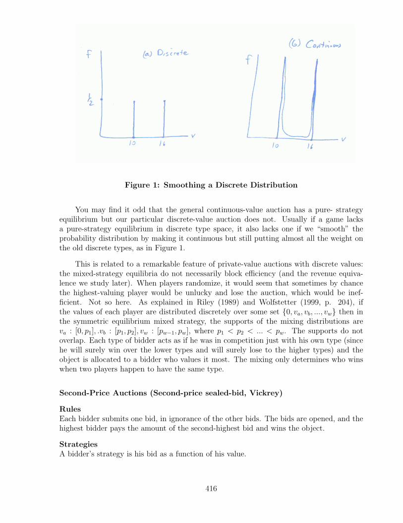
Figure 1: Smoothing a Discrete Distribution

You may find it odd that the general continuous-value auction has a pure- strategyequilibrium but our particular discrete-value auction does not. Usually if a game lacksa pure-strategy equilibrium in discrete type space, it also lacks one if we “smooth” theprobability distribution by making it continuous but still putting almost all the weight onthe old discrete types, as in Figure 1.

This is related to a remarkable feature of private-value auctions with discrete values:the mixed-strategy equilibria do not necessarily block efficiency (and the revenue equiva-lence we study later). When players randomize, it would seem that sometimes by chancethe highest-valuing player would be unlucky and lose the auction, which would be inef-ficient. Not so here. As explained in Riley (1989) and Wolfstetter (1999, p. 204), ifthe values of each player are distributed discretely over some set {0, va, vb, ..., vw} then inthe symmetric equilibrium mixed strategy, the supports of the mixing distributions areva : [0, p1], .vb : [p1, p2], vw : [pw−1, pw], where p1 < p2 < ... < pw. The supports do notoverlap. Each type of bidder acts as if he was in competition just with his own type (sincehe will surely win over the lower types and will surely lose to the higher types) and theobject is allocated to a bidder who values it most. The mixing only determines who winswhen two players happen to have the same type.

Second-Price Auctions (Second-price sealed-bid, Vickrey)

RulesEach bidder submits one bid, in ignorance of the other bids. The bids are opened, and thehighest bidder pays the amount of the second-highest bid and wins the object.

StrategiesA bidder’s strategy is his bid as a function of his value.

416

PayoffsThe winning bidder’s payoff is his value minus the second-highest bid. The losing bidders’payoffs are zero. The seller’s payoff is the second-highest-bid.

DiscussionSecond-price auctions are similar to ascending auctions. They are rarely used in reality,but are useful for modelling. Bidding one’s value is a weakly dominant strategy: a bidderwho bids less is no more likely to win the auction (and probably less likely, depending onf(v)), but he pays the same price— the second-highest-valuing player’s bid— if he doeswin. The structure of the payoffs is reminiscent of the Groves Mechanism of Section 10.4,because in both games a bidder’s strategy affects some major event (who wins the auction,or whether the project is undertaken), but his strategy affects his own payoff only via thatevent. In the auction’s symmetric equilibrium, each bidder bids his value and the winnerends up paying the second-highest value. If bidders know their own values, the outcomedoes not depend on risk neutrality.

One difference between ascending and second-price auctions is that second- price auc-tions have peculiar asymmetric equilibria because the actions in them are simultaneous.Consider a variant of the Ten-Sixteen Auction, in which each of two bidders’ values canbe 10 or 16, but where the realized values are common knowledge. Bidding one’s valueis a symmetric equilibrium, meaning that the bid function p(v) is the same for bothbidders: {p(v = 10) = 10, p(v = 16) = 16}. But there are asymmetric equilibria.

Consider the following equilibrium.

p1(v = 10) = 10 p1(v = 16) = 16

p2(v = 10) = 1 p2(v = 16) = 10(24)

Since Bidder 1 never bids less than 10, Bidder 2 knows that if v2 = 10 he can neverget a positive payoff, so he is willing to choose p2(v = 10) = 1. Doing so results in a saleprice of 1, for any p1 > 1, which is better for Bidder 1 and worse for the seller than a priceof 10, but Bidder 2 doesn’t care about their payoffs. In the same way, if v2 = 16, Bidder 2knows that if he bids 10 he will win if v1 = 10, but if v2 = 16 he would have to pay 16 towin and would earn a payoff of zero. He might as well bid 10 and earn his zero by losing. 1

Perhaps the seller’s fear of asymmetric equilibria like this is why Second- price auctionsare so rare. They have actually been used, though, in a computer operating system. Anoperating system must assign a computer’s resources to different tasks, and researchersat Xerox Corporation designed the Spawn system, under which users allocate “money”in a second-price auction for computer resources. See “Improving a Computer Network’sEfficiency,” The New York Times, p. 35 (29 March 1989).

Descending Auctions (Dutch)

1Trembling-hand perfectness, however, would rule out this kind of equilibrium. If Bidder 1 mighttremble and bid, for example, 4 by accident, Bidder 2 would not want to ever bid less than 4. Bidding lessthan one’s value is weakly dominated by bidding exactly one’s value– but Nash equilibrium strategies canbe weakly dominated, as we saw with the Bertrand Game in Chapter 3.

417

RulesThe seller announces a bid, which he continuously lowers until some bidder stops him andtakes the object at that price.

StrategiesA bidder’s strategy is when to stop the bidding as a function of his value.

PayoffsThe winner’s payoff is his value minus his bid. The losers’ payoffs are zero.

Discussion

The typical descending auction is strategically equivalent to the first-price auction,which means there is a one-to-one mapping between the strategy sets and the equilibriaof the two games. The reason for the strategic equivalence is that no relevant informationis disclosed in the course of the auction, only at the end, when it is too late to changeanybody’s behavior. In the first-price auction a bidder’s bid is irrelevant unless it is thehighest, and in the descending auction a bidder’s stopping price is irrelevant unless it isthe highest. The equilibrium price is calculated the same way for both auctions.

A descending auction does not have to be like a first-price auction as a matter of logic,though. Vickrey (1961) notes that a descending auction could be set up as a second-priceauction. When the first bidder presses his button, he primes an auction-ending buzzer thatdoes not goes off until a second bidder presses his button. In that case, the descendingauction would be strategically equivalent to a second-price auction. Economists almostalways mean “first- price descending auctions” when they use the term, however.

Descending–“Dutch”–auctions have been used in the Netherlands to sell flowers– seethe Aalsmeer auction website at http://www.vba.nl for information and photos. They havealso been used in Ontario to sell tobacco using a clock four feet in diameter marked withquarter-cent gradations. Each of six or so bidders has a stop button. The clock hand dropsa quarter-cent at a time, and the stop buttons are registered so that ties cannot occur(tobacco bidders need reflexes like race-car drivers). The farmer sellers watch from anadjoining room and can later reject the bids if they feel they are too low (a form of reserveprice) The clock is fast enough to sell 2,500,000 lb. per day (Cassady [1967, p. 200]).

Descending auctions are common in less obvious forms. Filene’s is one of the biggeststores in Boston, and Filene’s Basement is its most famous department. In the basementare a variety of marked-down items formerly in the regular store, each with a price anddate attached. The price customers pay at the register is the price on the tag minus adiscount which depends on how long ago the item was dated. As time passes and the itemremains unsold, the discount rises from 10 to 50 to 70 percent. The idea of predictabletime discounting has also been used by bookstores too (“Waldenbooks to Cut Some BookPrices in Stages in Test of New Selling Tactic,” The Wall Street Journal, March 29, 1988,p. 34).

All-Pay Auctions

418

RulesEach bidder places a bid simultaneously. The bidder with the highest bid wins, and eachbidder pays the amount he bid.

StrategiesA bidder’s strategy is his bid as a function of his value.

PayoffsThe winner’s payoff is his value minus his bid. The losers’ payoffs are the negative of theirbids.

DiscussionThe winning bid will be lower in the all-pay auction than under the other rules, becausebidders need a bigger payoff when they do win to make up for their negative payoffs whenthey lose. At the same time, since even the losing bidders pay something to the seller itis not obvious that the seller does badly (and in fact, it turns out to be just as good anauction rule as the others, in this simple risk-neutral context).

I do not know of the all-pay rule ever being used in a real auction, but it is a usefulmodelling tool because it models rent-seeking very well. When a number of companies lobbya politician for a privilege, they are in an all-pay auction because even the losers have paidby incurring the cost of lobbbying. When a number of companies pursue a patent, it is anall-pay auction because even the losers have incurred the cost of doing research.

The Equal-Value All-Pay Auction

Suppose each of the n bidders has the same value, v. That is not a very interestinggame for most of the auction rules, though it is true that for the second-price auction thereexists the strange asymmetric equilibrium {v, 0, 0, ....0}. Under the all-pay auction rule,however, this game is quite interesting. The equilibrium is in mixed strategies. This iseasy to see, because in any pure-strategy profile, either the maximum bid is less than v,in which case someone could deviate to p = v and increase his payoff; or one bidder bidsv and the rest bid at most p′ < v, in which case the high bidder will deviate to bid justabove p′.

419

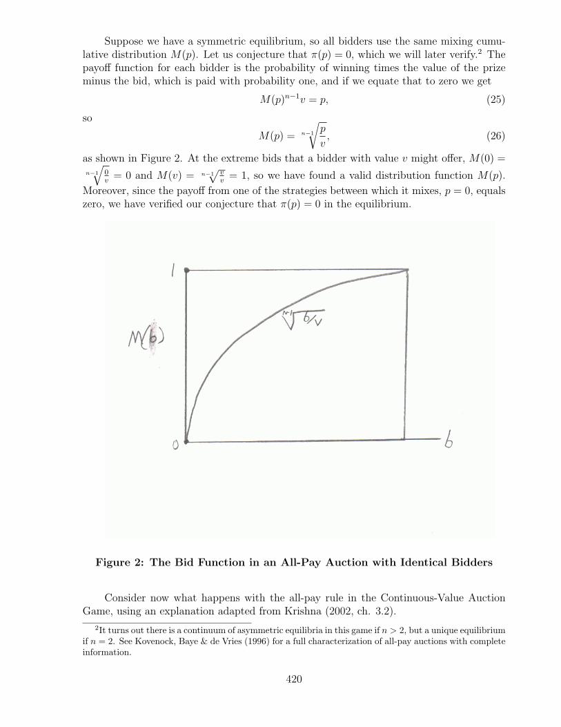
Suppose we have a symmetric equilibrium, so all bidders use the same mixing cumu-lative distribution M(p). Let us conjecture that π(p) = 0, which we will later verify.2 Thepayoff function for each bidder is the probability of winning times the value of the prizeminus the bid, which is paid with probability one, and if we equate that to zero we get

M(p)n−1v = p, (25)

so

M(p) = n−1

√p

v, (26)

as shown in Figure 2. At the extreme bids that a bidder with value v might offer, M(0) =n−1

√0v

= 0 and M(v) = n−1√

vv

= 1, so we have found a valid distribution function M(p).

Moreover, since the payoff from one of the strategies between which it mixes, p = 0, equalszero, we have verified our conjecture that π(p) = 0 in the equilibrium.

Figure 2: The Bid Function in an All-Pay Auction with Identical Bidders

Consider now what happens with the all-pay rule in the Continuous-Value AuctionGame, using an explanation adapted from Krishna (2002, ch. 3.2).

2It turns out there is a continuum of asymmetric equilibria in this game if n > 2, but a unique equilibriumif n = 2. See Kovenock, Baye & de Vries (1996) for a full characterization of all-pay auctions with completeinformation.

420

The Continuous-Value All-Pay Auction

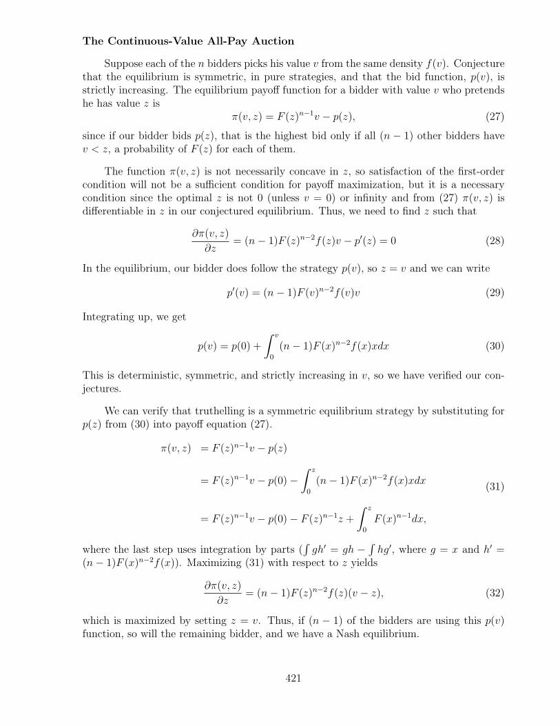
Suppose each of the n bidders picks his value v from the same density f(v). Conjecturethat the equilibrium is symmetric, in pure strategies, and that the bid function, p(v), isstrictly increasing. The equilibrium payoff function for a bidder with value v who pretendshe has value z is

π(v, z) = F (z)n−1v − p(z), (27)

since if our bidder bids p(z), that is the highest bid only if all (n − 1) other bidders havev < z, a probability of F (z) for each of them.

The function π(v, z) is not necessarily concave in z, so satisfaction of the first-ordercondition will not be a sufficient condition for payoff maximization, but it is a necessarycondition since the optimal z is not 0 (unless v = 0) or infinity and from (27) π(v, z) isdifferentiable in z in our conjectured equilibrium. Thus, we need to find z such that

∂π(v, z)

∂z= (n− 1)F (z)n−2f(z)v − p′(z) = 0 (28)

In the equilibrium, our bidder does follow the strategy p(v), so z = v and we can write

p′(v) = (n− 1)F (v)n−2f(v)v (29)

Integrating up, we get

p(v) = p(0) +

∫ v

0

(n− 1)F (x)n−2f(x)xdx (30)

This is deterministic, symmetric, and strictly increasing in v, so we have verified our con-jectures.

We can verify that truthelling is a symmetric equilibrium strategy by substituting forp(z) from (30) into payoff equation (27).

π(v, z) = F (z)n−1v − p(z)

= F (z)n−1v − p(0)−∫ z

0

(n− 1)F (x)n−2f(x)xdx

= F (z)n−1v − p(0)− F (z)n−1z +

∫ z

0

F (x)n−1dx,

(31)

where the last step uses integration by parts (∫

gh′ = gh −∫

hg′, where g = x and h′ =(n− 1)F (x)n−2f(x)). Maximizing (31) with respect to z yields

∂π(v, z)

∂z= (n− 1)F (z)n−2f(z)(v − z), (32)

which is maximized by setting z = v. Thus, if (n − 1) of the bidders are using this p(v)function, so will the remaining bidder, and we have a Nash equilibrium.

421

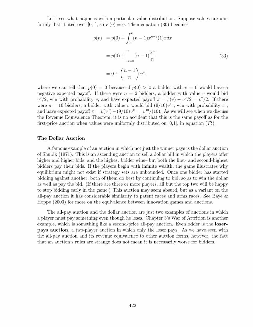
Let’s see what happens with a particular value distribution. Suppose values are uni-formly distributed over [0,1], so F (v) = v. Then equation (30) becomes

p(v) = p(0) +

∫ v

0

(n− 1)xn−2(1)xdx

= p(0) +

∣∣∣∣vx=0

(n− 1)xn

n

= 0 +

(n− 1

n

)vn,

(33)

where we can tell that p(0) = 0 because if p(0) > 0 a bidder with v = 0 would have anegative expected payoff. If there were n = 2 bidders, a bidder with value v would bidv2/2, win with probability v, and have expected payoff π = v(v) − v2/2 = v2/2. If therewere n = 10 bidders, a bidder with value v would bid (9/10)v10, win with probability v9,and have expected payoff π = v(v9)− (9/10)v10 = v10/(10). As we will see when we discussthe Revenue Equivalence Theorem, it is no accident that this is the same payoff as for thefirst-price auction when values were uniformly distributed on [0,1], in equation (??).

The Dollar Auction

A famous example of an auction in which not just the winner pays is the dollar auctionof Shubik (1971). This is an ascending auction to sell a dollar bill in which the players offerhigher and higher bids, and the highest bidder wins– but both the first- and second-highestbidders pay their bids. If the players begin with infinite wealth, the game illustrates whyequilibrium might not exist if strategy sets are unbounded. Once one bidder has startedbidding against another, both of them do best by continuing to bid, so as to win the dollaras well as pay the bid. (If there are three or more players, all but the top two will be happyto stop bidding early in the game.) This auction may seem absurd, but as a variant on theall-pay auction it has considerable similarity to patent races and arms races. See Baye &Hoppe (2003) for more on the equivalence between innovation games and auctions.

The all-pay auction and the dollar auction are just two examples of auctions in whicha player must pay something even though he loses. Chapter 3’s War of Attrition is anotherexample, which is something like a second-price all-pay auction. Even odder is the loser-pays auction, a two-player auction in which only the loser pays. As we have seen withthe all-pay auction and its revenue equivalence to other auction forms, however, the factthat an auction’s rules are strange does not mean it is necessarily worse for bidders.

422

All-pay auctions are a standard way to model rentseeking: imagine that n players eachexert e in effort simultaneously to get a prize worth V , the winner being whoever’s effort ishighest. Another common way to model rentseeking is as an auction in which the highestbidder has the best chance to win but lower bidders might win instead. Tullock (1980)started a literature on this in an article which was valuable despite a mistaken claim thatthe expected amount paid by the bidders might exceed the value of the prize. (See Baye,Kovenock & de Vries (1999) for a more recent analysis of this rent dissipation). Thereis no obvious way to model contests, and the functional form does matter to behavior, asJack Hirshleifer (1989) tells us. In the most popular functional form, P1 and P2 are theprobabilities of winning of the two players, e1 and e2 are their efforts, and R and θ areparameters which can be used to increase the probability that the high bidder wins or togive one player an advantage over the other. The victory function is then assumed to be

P1 =θeR

1

θeR1 + eR

2

and P2 =eR2

θeR1 + eR

2

(34)

If θ = 1 and R becomes large, this becomes close to the simple all-pay auction, becauseneither player has an advantage and the highest bidder wins with probability near one.

Once we depart from true auctions, however, the modeller must be careful about someseemingly obvious assumptions. Two bidders can simply refuse to enter the dollar auction,for example, but two countries have a harder time refusing to enter a situation in whichan arms race is tempting, though they can try to collude in keeping the bids small. It isalso often plausible that the size of the prize rises or falls with the bids– for example, whenthe contest is a mechanism used by a team to motivate its members to produce more (seeChung [1996]) or when the prize shrinks with effort because rent-seeking hurts the economy(see Alexeev & Leitzel [1996]).

13.3 Revenue Equivalence, Risk Aversion, and Uncertainty

We can now collect together the outcomes of these various auction rules and comparethem. We have seen that the first-price and descending auctions are strategically equivalent,so the payoffs to the bidders and seller will be the same under each rule regardless of whethervalues are private or common and whether the players are risk neutral or risk averse.

423

When values are private and independent, the second-price and ascending auctions arethe same in the sense that the bidder who values the object most highly wins and pays thesecond-highest of the values of all the bidders present, but the strategies are different inthe two auctions. In all five kinds of auctions, however, the seller’s expected revenue is thesame. This is the biggest result in auction theory: the Revenue Equivalence Theoremof Vickrey (1961). This has been variously generalized from Vickrey’s original statement(e.g., Klemperer (2004, p. 40), so there is no single Revenue Equivalence Theorem, butthey all share the same idea of payoffs being the same under various auction rules. Wewill look at two versions, a general one for auctions with particular properties and a morespecific one– a corollary, really– for the five auction rules just analyzed.

THE REVENUE EQUIVALENCE THEOREM. Let all players be risk-neutral with privatevalues drawn independently from the same atomless, strictly increasing distribution F (v)on [v, v]. If under either Auction Rule A1 or Auction Rule A2 it is true that:(a) The winner of the object is the player with the highest value; and(b) The lowest bidder type, v = v, has an expected payment of zero;then the symmetric equilibria of the two auction rules have the same expected payoffs foreach type of bidder and for the seller.

Proof. Let us represent the auction as the truthful equilibrium of a direct mechanism inwhich each bidder sends a message z of his type v and then pays an expected amount p(z).(The Revelation Principle says that we can do this.) By assumption (a), the probability thata player wins the object given that he chooses message z equals F (z)n−1, the probabilitythat all (n− 1) other players have values v < z. Let us denote this winning probability byG(z), with density g(z). Note that g(z) is well defined because we assumed that F (v) isatomless and everywhere increasing.

424

The expected payoff of any player of type v is the same, since we are restrictingourselves to symmetric equilibria. It equals

π(z, v) = G(z)v − p(z). (35)

The first-order condition with respect to the player’s choice of type message z (which wecan use because neither z = 0 nor z = v is the optimum if condition (a) is to be true) is

dπ(z; v)

dz= g(z)v − dp(z)

dz= 0, (36)

sodp(z)

dz= g(z)v. (37)

We are looking at a truthful equilibrium, so we can replace z with v:

dp(v)

dv= g(v)v. (38)

Next, we integrate (38) over all values from zero to v, adding p(v) as the constant ofintegration:

p(v) = p(v) +

∫ v

v

g(x)xdx. (39)

We can use (39 to substitute for p(v) in the payoff equation (35), which becomes, afterreplacing z with v and setting p(v) = 0 because of assumption (b),

π(v, v) = G(v)v −∫ v

v

g(x)xdx. (40)

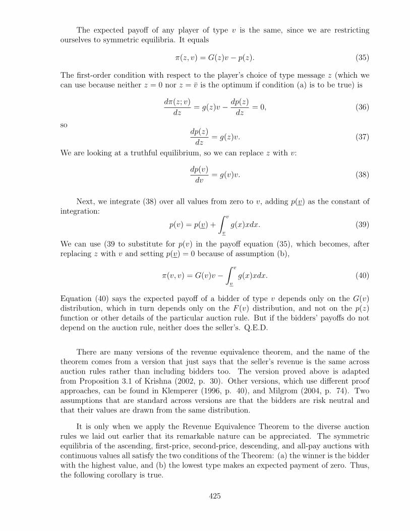
Equation (40) says the expected payoff of a bidder of type v depends only on the G(v)distribution, which in turn depends only on the F (v) distribution, and not on the p(z)function or other details of the particular auction rule. But if the bidders’ payoffs do notdepend on the auction rule, neither does the seller’s. Q.E.D.

There are many versions of the revenue equivalence theorem, and the name of thetheorem comes from a version that just says that the seller’s revenue is the same acrossauction rules rather than including bidders too. The version proved above is adaptedfrom Proposition 3.1 of Krishna (2002, p. 30). Other versions, which use different proofapproaches, can be found in Klemperer (1996, p. 40), and Milgrom (2004, p. 74). Twoassumptions that are standard across versions are that the bidders are risk neutral andthat their values are drawn from the same distribution.

It is only when we apply the Revenue Equivalence Theorem to the diverse auctionrules we laid out earlier that its remarkable nature can be appreciated. The symmetricequilibria of the ascending, first-price, second-price, descending, and all-pay auctions withcontinuous values all satisfy the two conditions of the Theorem: (a) the winner is the bidderwith the highest value, and (b) the lowest type makes an expected payment of zero. Thus,the following corollary is true.

425

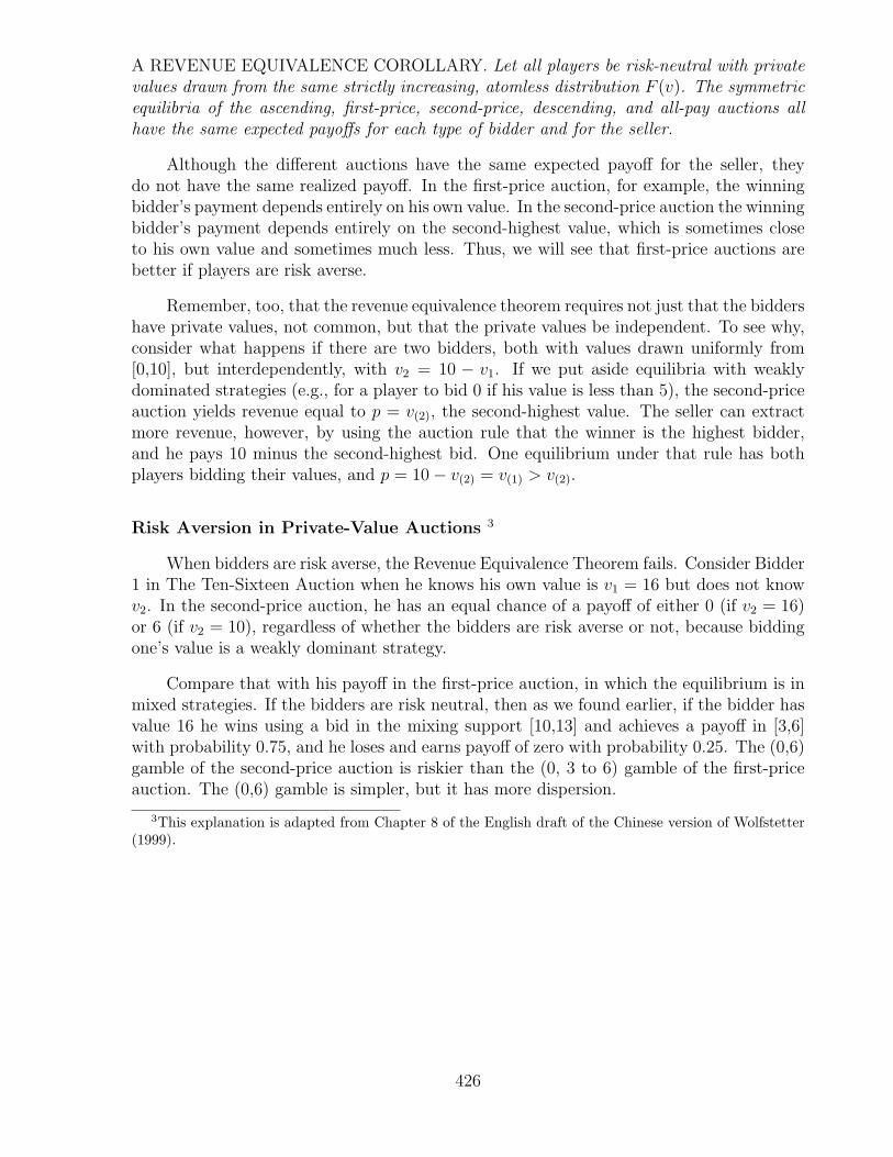
A REVENUE EQUIVALENCE COROLLARY. Let all players be risk-neutral with privatevalues drawn from the same strictly increasing, atomless distribution F (v). The symmetricequilibria of the ascending, first-price, second-price, descending, and all-pay auctions allhave the same expected payoffs for each type of bidder and for the seller.

Although the different auctions have the same expected payoff for the seller, theydo not have the same realized payoff. In the first-price auction, for example, the winningbidder’s payment depends entirely on his own value. In the second-price auction the winningbidder’s payment depends entirely on the second-highest value, which is sometimes closeto his own value and sometimes much less. Thus, we will see that first-price auctions arebetter if players are risk averse.

Remember, too, that the revenue equivalence theorem requires not just that the biddershave private values, not common, but that the private values be independent. To see why,consider what happens if there are two bidders, both with values drawn uniformly from[0,10], but interdependently, with v2 = 10 − v1. If we put aside equilibria with weaklydominated strategies (e.g., for a player to bid 0 if his value is less than 5), the second-priceauction yields revenue equal to p = v(2), the second-highest value. The seller can extractmore revenue, however, by using the auction rule that the winner is the highest bidder,and he pays 10 minus the second-highest bid. One equilibrium under that rule has bothplayers bidding their values, and p = 10− v(2) = v(1) > v(2).

Risk Aversion in Private-Value Auctions 3

When bidders are risk averse, the Revenue Equivalence Theorem fails. Consider Bidder1 in The Ten-Sixteen Auction when he knows his own value is v1 = 16 but does not knowv2. In the second-price auction, he has an equal chance of a payoff of either 0 (if v2 = 16)or 6 (if v2 = 10), regardless of whether the bidders are risk averse or not, because biddingone’s value is a weakly dominant strategy.

Compare that with his payoff in the first-price auction, in which the equilibrium is inmixed strategies. If the bidders are risk neutral, then as we found earlier, if the bidder hasvalue 16 he wins using a bid in the mixing support [10,13] and achieves a payoff in [3,6]with probability 0.75, and he loses and earns payoff of zero with probability 0.25. The (0,6)gamble of the second-price auction is riskier than the (0, 3 to 6) gamble of the first-priceauction. The (0,6) gamble is simpler, but it has more dispersion.

3This explanation is adapted from Chapter 8 of the English draft of the Chinese version of Wolfstetter(1999).

426

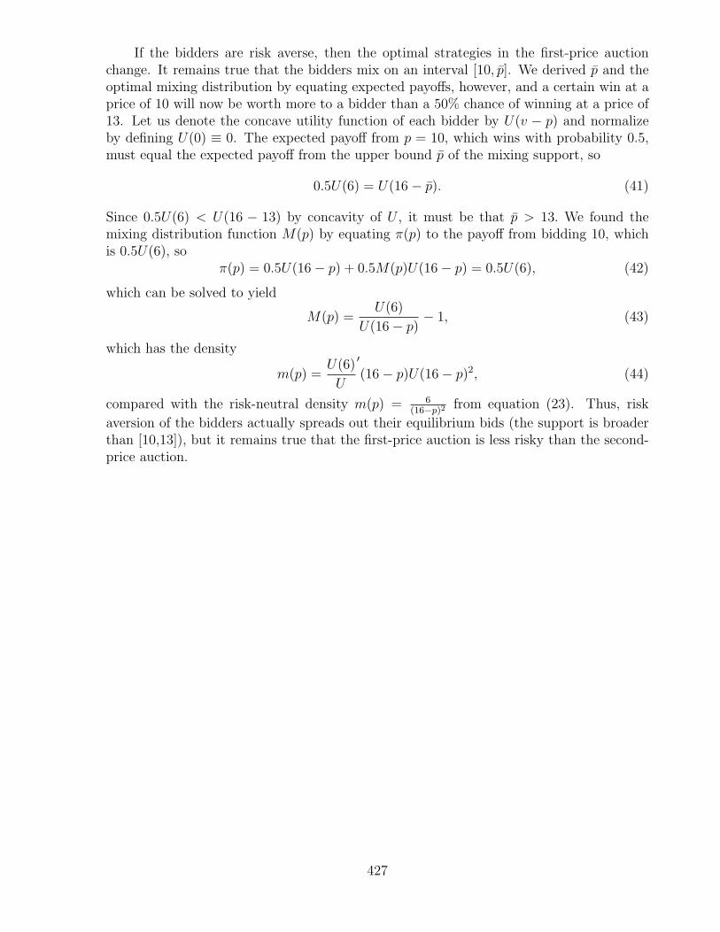
If the bidders are risk averse, then the optimal strategies in the first-price auctionchange. It remains true that the bidders mix on an interval [10, p]. We derived p and theoptimal mixing distribution by equating expected payoffs, however, and a certain win at aprice of 10 will now be worth more to a bidder than a 50% chance of winning at a price of13. Let us denote the concave utility function of each bidder by U(v − p) and normalizeby defining U(0) ≡ 0. The expected payoff from p = 10, which wins with probability 0.5,must equal the expected payoff from the upper bound p of the mixing support, so

0.5U(6) = U(16− p). (41)

Since 0.5U(6) < U(16 − 13) by concavity of U , it must be that p > 13. We found themixing distribution function M(p) by equating π(p) to the payoff from bidding 10, whichis 0.5U(6), so

π(p) = 0.5U(16− p) + 0.5M(p)U(16− p) = 0.5U(6), (42)

which can be solved to yield

M(p) =U(6)

U(16− p)− 1, (43)

which has the density

m(p) =U(6)

U

′

(16− p)U(16− p)2, (44)

compared with the risk-neutral density m(p) = 6(16−p)2

from equation (23). Thus, risk

aversion of the bidders actually spreads out their equilibrium bids (the support is broaderthan [10,13]), but it remains true that the first-price auction is less risky than the second-price auction.

427

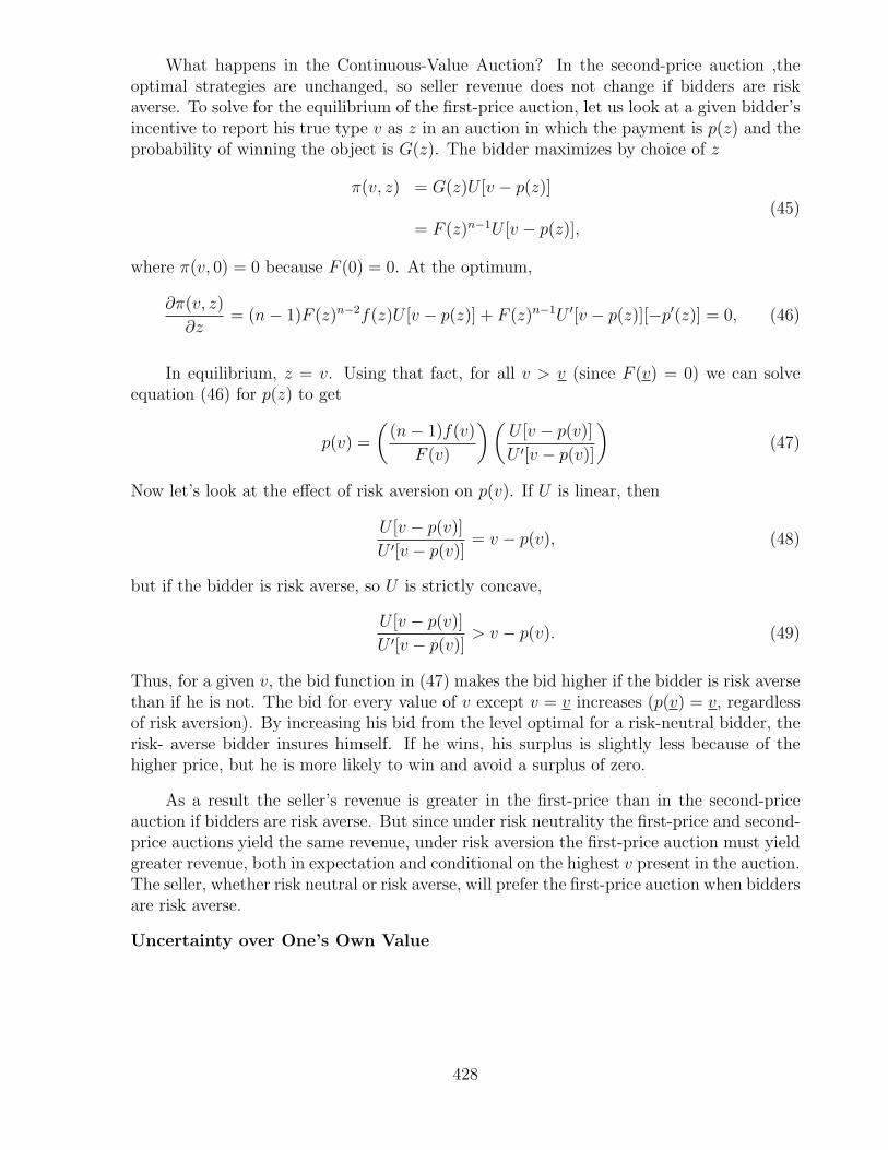
What happens in the Continuous-Value Auction? In the second-price auction ,theoptimal strategies are unchanged, so seller revenue does not change if bidders are riskaverse. To solve for the equilibrium of the first-price auction, let us look at a given bidder’sincentive to report his true type v as z in an auction in which the payment is p(z) and theprobability of winning the object is G(z). The bidder maximizes by choice of z

π(v, z) = G(z)U [v − p(z)]

= F (z)n−1U [v − p(z)],(45)

where π(v, 0) = 0 because F (0) = 0. At the optimum,

∂π(v, z)

∂z= (n− 1)F (z)n−2f(z)U [v − p(z)] + F (z)n−1U ′[v − p(z)][−p′(z)] = 0, (46)

In equilibrium, z = v. Using that fact, for all v > v (since F (v) = 0) we can solveequation (46) for p(z) to get

p(v) =

((n− 1)f(v)

F (v)

)(U [v − p(v)]

U ′[v − p(v)]

)(47)

Now let’s look at the effect of risk aversion on p(v). If U is linear, then

U [v − p(v)]

U ′[v − p(v)]= v − p(v), (48)

but if the bidder is risk averse, so U is strictly concave,

U [v − p(v)]

U ′[v − p(v)]> v − p(v). (49)

Thus, for a given v, the bid function in (47) makes the bid higher if the bidder is risk aversethan if he is not. The bid for every value of v except v = v increases (p(v) = v, regardlessof risk aversion). By increasing his bid from the level optimal for a risk-neutral bidder, therisk- averse bidder insures himself. If he wins, his surplus is slightly less because of thehigher price, but he is more likely to win and avoid a surplus of zero.

As a result the seller’s revenue is greater in the first-price than in the second-priceauction if bidders are risk averse. But since under risk neutrality the first-price and second-price auctions yield the same revenue, under risk aversion the first-price auction must yieldgreater revenue, both in expectation and conditional on the highest v present in the auction.The seller, whether risk neutral or risk averse, will prefer the first-price auction when biddersare risk averse.

Uncertainty over One’s Own Value

428

We have seen that when bidders are risk averse, revenue equivalence fails because thesecond-price auction is riskier than the first-price auction. By the same reasoning, theascending auction is riskier, and by strategic equivalence the descending auction is the sameas the first-price. Risk aversion matters for different reasons if the bidders do not knowtheir values precisely. As we will see later, in the context of common values, uncertaintyover one’s own value will generate conservative bidding behavior for the strategic reasonof the “Winner’s Curse”— a reason which applies whether bidders are risk averse or not—and because of the “Linkage Principle” of Milgrom & Weber (1982). Value uncertaintyalso has a simpler effect that is driven by risk aversion and applies even in independentprivate-value auctions: buying a good of uncertain value is instrinsically risky, whetherbuying it by auction or by a posted price.

Consider the following question:

If the seller can reduce bidder uncertainty over the value of the object being auctioned,should he do so?

Let us assume that the seller can precommit to reveal both favorable information andunfavorable information, since of course he would like best to reveal only information thatraises bidder estimates of the object’s value (though the unravelling effect of Chapter 10might undo such a strategy). It is often plausible that the seller can set up an auctionsystem which reduces uncertainty – say, by a regular policy of allowing bidders to examinethe goods before the auction begins. Let us build a model to show the effect of such apolicy.

Suppose there are n bidders, each with a private value, in an ascending auction. Eachmeasures his private value v with an independent error ε > 0. This error is with equalprobability −x, +x or 0. The bidders have diffuse priors, so they take all values of v tobe equally likely, ex ante. Let us denote a bidder’s measured value by v = v + ε, which isan unbiased estimate of v. In the ascending auctions we have been studying so far, whereε = 0, the optimal bid ceiling was v. Now, when ε > 0, what bid ceiling should be used bya bidder with utility function U(v − p)?

If the bidder wins the auction and pays p for the object, his expected utility at thatpoint is

π(p) =U([v − x]− p)

3+

U(v − p)

3+

U([v + x]− p)

3(50)

If he is risk neutral, this yields him a payoff of zero if p = v, and winning at any lowerprice would yield a positive payoff. This is true because we can write U(v− p) = v− p and

π(risk neutral, p = v) =([v − x]− v)

3+

(v − v)

3+

(v + x− v)

3= 0. (51)

Thus, under risk neutrality uncertainty over one’s own value does not affect the optimalstrategy, except that the bidder’s bid ceiling is his expected value for the object rather thanhis value. Adverse selection aside, there is no reason for the seller to try to improve bidderinformation.

429

If the bidder is risk averse, however, then the utility function U is concave and

U([v − x]− p)

3+

U([v + x]− p)

3<

(2

3

)U(v − p), (52)

so his expected payoff in equation (50) is less than U(v − p), and if p = v his payoff is lessthan U(0). A risk-averse bidder will have a negative expected payoff from paying his bidceiling unless it is strictly less than his estimated value.

Notice that the seller does not have control over all the elements of the model. Theseller can often choose the auction rules unilaterally. This includes not just how bids aremade, but such things as whether the bidders get to know how many potential bidders arein the auction, whether the seller himself is allowed to bid, and so forth. Also, the sellercan decide how much information to release about the goods. The seller cannot, however,decide whether the bidders are risk averse or not, or whether they have common or privatevalues, no more than he can choose what their values are for the good he is selling. All ofthose assumptions concern the utility functions of the bidders. At best, the seller can dothings such as choose to produce goods to sell at the auction which have common valuesinstead of private values.

An error I have often seen is to think that the presence of uncertainty over one’s valuealways causes the Winner’s Curse that we will shortly examine. It does not, unless theauction is in common values; uncertainty over one’s value is a necessary but not sufficientcondition for the Winner’s Curse. It is true that risk-averse bidders should not bid ashigh as their value estimates if they are uncertain about them, even if the auction is inprivate values. That sounds a lot like a Winner’s Curse, but the reason for the discountedbids is completely different, depending as it does on risk aversion. If bidders are uncertainabout value estimates but they are risk neutral, their dominant strategy is still to bid upto their value estimates. If the Winner’s Curse is present, even if a bidder is risk-neutralhe discounts his bid because if he wins, on average his estimate will be greater than thevalue.

13.4 Reserve Prices and the Marginal Revenue Approach

A reserve price p∗ is a bid put in by the seller, secretly or openly, before the auctionbegins, which commits him not to sell the object if nobody bids more than p∗. The sellerwill often find that a reserve price can increase his payoff. If he does, it turns out that hewill choose a reserve price strictly greater than his own value: p∗ > vs. To see this, wewill use the marginal revenue approach to auctions, an approach developed in Bulow &Roberts (1989) for risk-neutral private values, and Bulow & Klemperer (1996) for commonvalues and risk aversion. This approach compares the seller in an auction to an ordinarymonopolist who sells using a posted price. We start with an auction to just one bidder, thenextend the idea to an auction with multiple bidders, and finally return to the surprisingsimilarity between an auction with one bidder and a monopoly selling to a continuum ofbidders using a posted price.

1. One Bidder. If there is just one bidder, the seller will do badly in any of the auctionrules we have discussed so far. The single bidder would bid p1 = 0 and win.

430

The situation is really better suited to bargaining or simple monopoly than to anauction. The seller could use an auction, but a standard auction yields him zero revenue.so posting a price offer to the bidder makes more sense. If the auction has a reserve price,however, it can be equivalent to posting a price, just as in bargaining the making of a singletake-it-or-leave-it offer of p∗ is equivalent to posting a price.

What should the offer p∗ be? Let the bidder have value distribution F (v) on [v, v] which isdifferentiable and strictly increasing, so the density f(v) is always positive. Let the sellervalue the object at vs ≥ v. The seller’s payoff is

π(p∗) = Pr(p∗ < v)(p∗ − vs) + Pr(p∗ > v)(0)

= [1− F (p∗)](p∗ − vs).(53)

This has first-order-condition

dπ(p∗)

dp∗= [1− F (p∗)]− f(p∗)[p∗ − vs] = 0. (54)

On solving (54) for for p∗ we get

p∗ = vs +

(1− F (p∗)

f(p∗)

). (55)

The optimal take-it-or-leave-it offer, the “reserve price” p∗ satisfies equation (55). Thereserve price is strictly greater than the seller’s value for the object (p∗ > vs) unless thesolution is such that F (p∗) = 1 because the optimal reserve price is the greatest possiblebidder value, in which case the object has probability zero of being sold. One reason to usea reserve price is so the seller does not sell an object for a price worth less than its valueto him, but that is not all that is going on.4

2. Multiple Bidders. Now let there be n bidders, all with values distributed indepen-dently by F (v). Denote the bidders with the highest and second-highest values as Bidders1 and 2. The seller’s payoff in a second-price auction is

π(p∗) = Pr(p∗ > v1)(0) + Pr(v2 < p∗ < v1)(p∗ − vs) + Pr(p∗ < Ev2 < v1)(v2 − vs)

=

∫ p∗

v1=v

f(v1)(0)dv1 +

∫ v

v1=p∗

(∫ p∗

v2=v

(p∗ − vs)f(v2)dv2 +

∫ v1

v2=p∗(v2 − vs)f(v2)dv2

)f(v1)dv1

(56)This expression integrates over two random variables. First, it matters whether v1 is greaterthan or less than p∗, the outer integrals. Second, it matters whether v2 is less than p∗ ornot, the inner integrals.

4The second-order condition for the problem is d2π(p∗)dp∗2 = −2f(p∗)+f ′(p∗)[p∗−vs] ≤ 0. This might well be

false, and in any case several values of p∗ might satisfy equation (55) so it is only a necessary condition, not asufficient one. Another way to see that p∗ > vs is to observe that dπ(p∗=vs)

dp∗ = [1−F (vs)−f(vs)[vs−vs] > 0,so p∗ should be increased beyond vs.

431

Now differentiate equation (56) to find the optimal reserve price p∗ using Leibniz’sintegral rule (given in the Mathematical Appendix):

dπ(p∗)

dp∗= 0 +−f(p∗)

(∫ p∗

v2=v

(p∗ − vs)f(v2)dv2 +

∫ p∗

v2=p∗(v2 − vs)f(v2)dv2

)

+

∫ v

v1=p∗

((p∗ − vs)f(p∗)− (p∗ − vs)f(p∗) +

∫ p∗

v2=v

f(v2)dv2

)f(v1)dv1

= −f(p∗)

(∫ p∗

v2=v

(p∗ − vs)f(v2)dv2 + 0

)+

∫ v

v1=p∗

(∫ p∗

v2=v

f(v2)dv2

)f(v1)dv1

= −f(p∗)F (p∗)(p∗ − vs) + (1− F (p∗))F (p∗) = 0(57)

Dividing by F , the last line of expression (57) implies that

p∗ = vs +1− F (p∗)

f(p∗), (58)

just what we found in equation (55) for the one-bidder case. Remarkably, the optimalreserve price is unchanged! Moreover, equation (58) applies to any number of bidders, notjust n = 2. Only Bidders 1 and 2 show up in the equations we used in the derivation, butthat is because they are the only ones to affect the result in a second-price auction.

In fact, only the highest-valuing bidder matters to the optimal reserve price. Thereserve price only affects the winning price if the second-highest- valuing bidder happensto have a rather low value. Conditioning on that, Bidder 1 would bid low if there were noreserve price– it is almost as if he faced no competition. But the seller, conditioning onthat value being low, would want to set a reserve price so that Bidder 1 must pay more.Since the reserve price only matters if all but one of the bidders have low values, it doesn’tmatter whether “all but one” is 99 or 0. Conditioning on all but one bidder having lowvalues, the seller is conditioning on the game having only one bidder who matters.

432

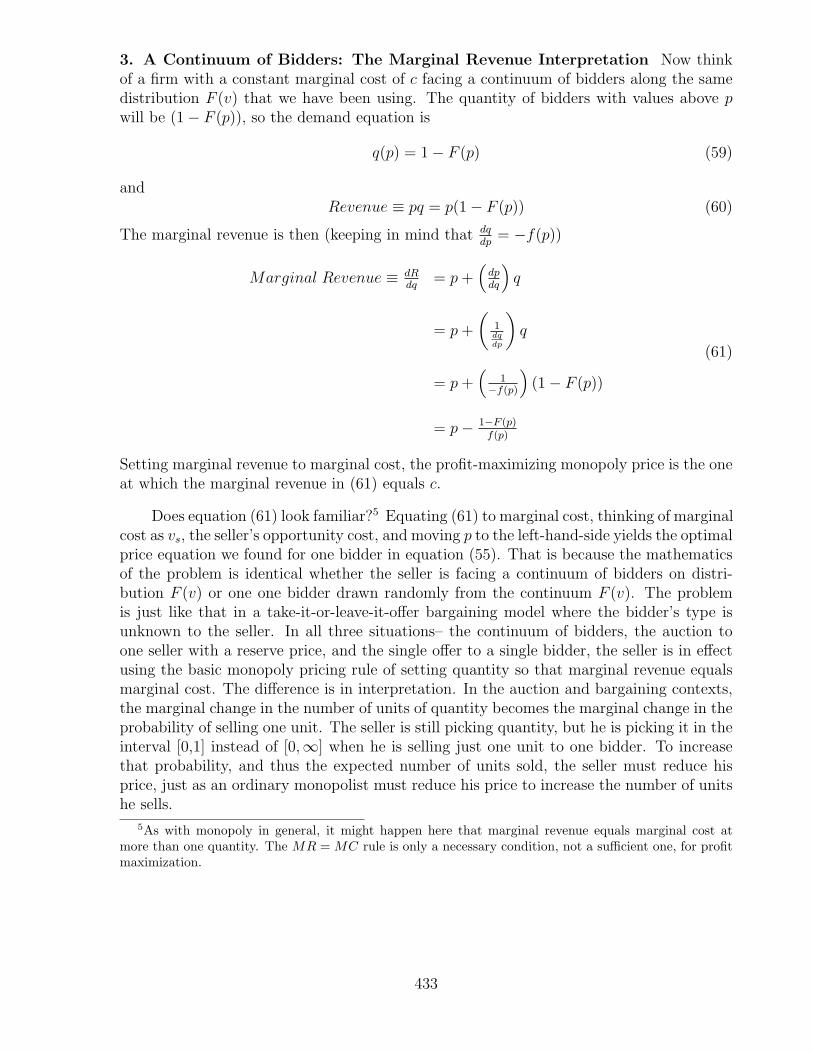
3. A Continuum of Bidders: The Marginal Revenue Interpretation Now thinkof a firm with a constant marginal cost of c facing a continuum of bidders along the samedistribution F (v) that we have been using. The quantity of bidders with values above pwill be (1− F (p)), so the demand equation is

q(p) = 1− F (p) (59)

andRevenue ≡ pq = p(1− F (p)) (60)

The marginal revenue is then (keeping in mind that dqdp

= −f(p))

Marginal Revenue ≡ dRdq

= p +(

dpdq

)q

= p +

(1dqdp

)q

= p +(

1−f(p)

)(1− F (p))

= p− 1−F (p)f(p)

(61)

Setting marginal revenue to marginal cost, the profit-maximizing monopoly price is the oneat which the marginal revenue in (61) equals c.

Does equation (61) look familiar?5 Equating (61) to marginal cost, thinking of marginalcost as vs, the seller’s opportunity cost, and moving p to the left-hand-side yields the optimalprice equation we found for one bidder in equation (55). That is because the mathematicsof the problem is identical whether the seller is facing a continuum of bidders on distri-bution F (v) or one one bidder drawn randomly from the continuum F (v). The problemis just like that in a take-it-or-leave-it-offer bargaining model where the bidder’s type isunknown to the seller. In all three situations– the continuum of bidders, the auction toone seller with a reserve price, and the single offer to a single bidder, the seller is in effectusing the basic monopoly pricing rule of setting quantity so that marginal revenue equalsmarginal cost. The difference is in interpretation. In the auction and bargaining contexts,the marginal change in the number of units of quantity becomes the marginal change in theprobability of selling one unit. The seller is still picking quantity, but he is picking it in theinterval [0,1] instead of [0,∞] when he is selling just one unit to one bidder. To increasethat probability, and thus the expected number of units sold, the seller must reduce hisprice, just as an ordinary monopolist must reduce his price to increase the number of unitshe sells.

5As with monopoly in general, it might happen here that marginal revenue equals marginal cost atmore than one quantity. The MR = MC rule is only a necessary condition, not a sufficient one, for profitmaximization.

433

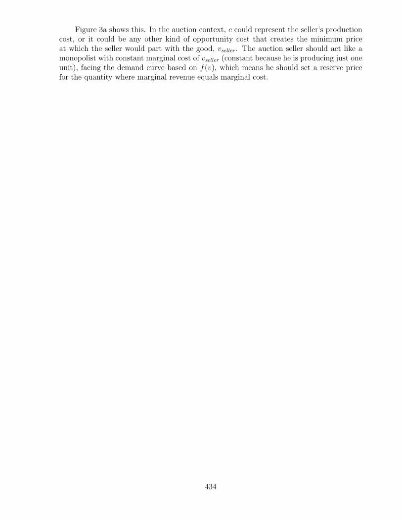
Figure 3a shows this. In the auction context, c could represent the seller’s productioncost, or it could be any other kind of opportunity cost that creates the minimum priceat which the seller would part with the good, vseller. The auction seller should act like amonopolist with constant marginal cost of vseller (constant because he is producing just oneunit), facing the demand curve based on f(v), which means he should set a reserve pricefor the quantity where marginal revenue equals marginal cost.

434

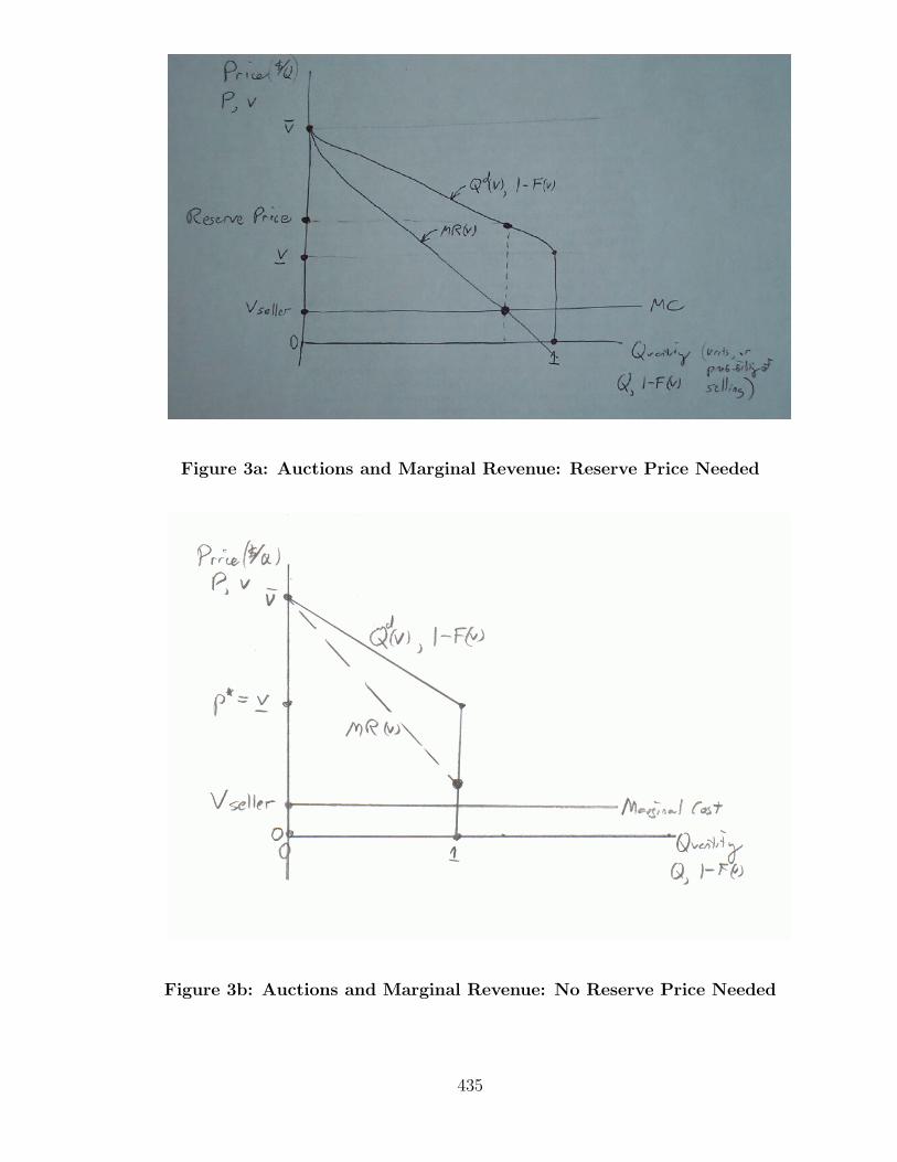
Figure 3a: Auctions and Marginal Revenue: Reserve Price Needed

Figure 3b: Auctions and Marginal Revenue: No Reserve Price Needed

435

The optimal reserve price will always be positive. In Figure 3a, even if vs were zeroinstead of positive, the curves are such that the reserve price should be positive, eventhough the probability of making a sale would then equal one. This corresponds to theidea that a monopolist will always raise the price above marginal cost, even though incertain situations (such as the curves in Figure 3b) he will not reduce output below thecompetitive level and a reserve price is redundant.

If output is reduced below the competitive level, the outcome is inefficient, somethingtrue both in conventional monopoly and here. Here, output is inefficiently low if no saletakes place of the one unit even though v > vs for some bidder. In that case, what theseller has done is to inefficiently reduce the expected output to below the one unit he hasavailable, resulting in an expected welfare loss equal to the area of a triangle, just as inconventional monopoly.

Unlike a conventional monopoly, there is a possibility of inefficient “overproduction”in an auction. That happens if the sale takes place even though no bidder values the goodas much as the seller: v < vs for the winning bidder. A positive reserve price, therefore, canhelp efficiency rather than hurt it. All the five auction forms — first-price, second-price,descending, ascending, and all-pay— can be efficient in a private-value setting, but onlyif the reserve price is set not at the profit-maximizing level but at p∗ = vs. We have alsoshown, however, that without a reserve price greater than vs, none of the five auction rulesis optimal for the seller. With the addition of an optimal reserve price, though, it can beshown (though we will not do so here) that in simple settings the seller need use no morecomplicated auction rules than one of the five we have studied.

In more complicated settings, of course, things do get more complicated, and thereis the possibility of inefficiency not just because the object is not sold at all, but becauseit might be sold to the “wrong” bidder (that is, not to the bidder who values it most). Ihave already mentioned that this can happen in asymmetric auctions, where the biddershave values drawn from different distributions instead of just one F (v). It could happen

that for two bidders,(

1−F1(v)f1(v)

)>(

1−F2(v)f2(v)

), in which case our rule for setting p∗ becomes

ambiguous– which bidder’s F function should we use? In such cases, the seller does bestif he biases the auction rules in favor of Bidder 2, who will then sometimes win even ifv2 < v1. A similar problem can arise if F is an unusual distribution, for which higher vdoes not imply that (v − 1−F (v)

f(v)) is higher. For more on the intricacies of such situations,

see Myerson (1981) or Bulow & Roberts (1989).

Hindering Bidder Collusion

The choice of auction rule can matter for another reason which comes to mind now thatwe have been discussing the seller as monopolist: the bidders may act as a monopsonist bycolluding. If the bidders can cooperate as if they were one bidder, we are in the situationjust described of an auction to one bidder, where use of a reserve price is critical and wherethe information-eliciting benefit of an auction to the seller evaporates. If the bidders try tocollude but remain selfish, however, the choice of an auction rule can make the differencebetween successful collusion and failure for them. Some auction rules are more vulnerableto collusion than others.

436

Robinson (1985) has pointed out that whether the auction is private-value or common-value, the first-price auction is superior to the second-price or ascending auctions for deter-ring collusion among bidders. (See, too, Graham & Marshall [1987]). Consider a bidder’scartel in which bidder Smith has a private value of 20, the other bidders’ values are each18, and they agree that everybody will bid 5 except Smith, who will bid 6. (We will notconsider the rationality of this choice of bids, which might be based on avoiding legal penal-ties.) In an ascending auction this is self- enforcing, because if somebody cheats and bids7, Smith is willing to go all the way up to 20 and the cheater will end up with no gainfrom his deviation. Enforcement is also easy in a second-price auction, because the cartelagreement can be that Smith bids 20 and everyone else bids 6, and if anyone cheats andbids higher than 6 he still loses unless he bids 20 or more.

Unlike in a ascending or second-price auction, however, in a first-price auction thebidders have a strong temptation to cheat. The bid p′ that the colluders would choose forSmith would be lower than p′ = 20, since he would have to pay his bid, but if p′ is anythingless than the other bidders’ value of 18 any one of them could gain by deviating to bidmore than p′ and win.

Thus, the seller should use a first-price auction if he fears collusion. Even then, cheatingwill be a problem if the game is repeated, and where collusive “bidding rings” are mostoften found is in markets where the same bidders meet over and over in auctions forsimilar objects. Thus, antique auctions are notorious for collusion among bidders who areprofessional antique dealers (and thus are “regulars” at the auctions and meet repeatedly).A similar problem arises when the same highway contractors repeatedly compete with eachother in bidding for who will carry out a government job at the lowest cost. A similarexample, described in the book by Sultan (1974), is the Electric Conspiracy of the 1950’s,in which antitrust authorities found and prosecuted collusion among executives in a fewlarge companies in bidding for electrical generating equipment contracts.

13.5 Common-Value Auctions and the Winner’s Curse

In Section 13.1 we distinguished private-value auctions from common-value auctions, inwhich the bidders all have the same value for the object but their value estimates may differ.All five sets of rules discussed there can be used for common-value auctions, but the optimalstrategies change. In common- value auctions, each bidder can extract useful informationabout the object’s value to himself from the bids of the other bidders. Surprisingly enough,a bidder can use the information from other bidders’ bids even in a sealed-bid auction, aswill be explained below.

437

A common-value auction in which all the bidders knew the value would not be veryinteresting–or very different from a private-value auction— but more commonly the biddersmust estimate the common value. The obvious strategy, especially following our discussionof private-value auctions, is for a risk- neutral bidder to bid up to his unbiased estimateof the value. But this strategy makes the winner’s payoff negative, because the winneris the bidder who has made the largest positive error in his estimate. The bidders whounderestimated the number of pennies lose the auction, but their payoff equals zero, whichthey would receive even if the true value were common knowledge. Only the winner suffersfrom his estimation error: he has stumbled into the Winner’s Curse, a phenomenon firstdescribed in Rothkopf (1969) and Wilson (1969).

When some bidders are better informed than others, the Winner’s Curse becomeseven more severe. Naturally if a bidder knows that he is the worst informed, he should becautious. Anyone, for example, who outbids 50 experts on the value of an object to win anauction should worry about why all the experts bid less. But the presence of the poorlyinformed bidder also increases the danger for the experts. Any experts who wins not justagainst 49 equally well-informed experts but also against a naive bidder who might wellhave made a large overestimation error and bid too high should worry too.

Once bidders recognize the possibility of the Winner’s Curse and adjust their biddingstrategies, the winner will no longer have to regret his victory. Having adjusted by scalingdown their bids to be lower than their unbiased estimates, the winner may still be thebidder with the biggest overestimation error, but the winning bid can still be less than thetrue value. Thus, the problem is to decide how much less than one’s value estimate to bid.

The mental process is a little like deciding how much to bid in a private- value, first-price auction. There, a bidder wants to bid less than his value, but he also wants to win ifhe can do so cheaply enough. He therefore tries to estimate the value of the second-highestbid conditional upon himself having the highest value and winning. In a common-valueauction a bidder’s first step is to use similar mathematics, but to estimate his own valueconditional upon winning the auction, not the second-highest value.

One way to think about a bidder’s conditional estimate is to think about it as aconditional bid. The bidder knows that if he wins using his unbiased estimate, he probablybid too high, so after winning with such a bid he would like to retract it. Intead, he wouldlike to submit a bid of [X if I lose, but (X − Y ) if I win], where X is his value estimateconditional on losing and (X−Y ) is his estimate conditional on winning— a lower estimate,since winning implies his overestimation error was the biggest of anybody’s. If he still wonwith a bid of (X − Y ) he would be happy. If he lost, he would be relieved. But Smith canachieve the same effect by simply submitting the bid (X−Y ) in the first place, since whenhe loses, the size of his bid is irrelevant.

438

Another way to look at the Winner’s Curse is based on the Milgrom definition of“bad news” (Milgrom [1981b], appendix b). Suppose the government is auctioning off themineral rights to a plot of land with common value v and that bidder i has value estimatevi. Suppose also that the bidders are identical in everything but their value estimates,which are based on the various information sets Nature has assigned them, and that theequilibrium is symmetric, so the equilibrium bid function p(vi) is the same for each bidder.If Bidder 1 wins with a bid p(v1) that is based on his prior value estimate v1, his posteriorvalue estimate v1 is

v1 = E(V |v1, p(v2) < p(v1), . . . , p(vn) < p(v1)). (62)

The news that p(v2) < ∞ would be neither good nor bad, since it conveys no information.The information that p(v2) < p(v1), however, is bad news, since it rules out values of pmore likely to be produced by large values of v2. In fact, the lower the winning value ofp(v1), the worse is the news of having won. Hence,

v1 < E(V |v1) = v1, (63)

and if Bidder 1 had bid p(v1) = v1 he would immediately regret having won. If his winningbid were enough below v1, however, he would be pleased to win.

Deciding how much to scale down the bid is a hard problem because the amount de-pends on how much all the other bidders scale down. In a second-price auction a biddercalculates the value of v1 using equation (62), but that equation hides considerable com-plexity under the disguise of the term p(v2), which is itself calculated as a function of p(v1)using an equation like (62).

Oil Tracts and the Winner’s Curse

The best known example of the Winner’s Curse is from bidding for offshore oil tracts.Offshore drilling can be unprofitable even if oil is discovered, because something mustbe paid to the government for the mineral rights. Physicists Capen, Clapp & Campbellsuggested in a 1971 paper in the Journal of Petroleum Engineering that bidders’ ignoranceof what they termed “the Winner’s Curse” caused overbidding in US government auctionsof the 1960s. If the oil companies had bid close to what their engineers estimated the tractswere worth, rather than scaling down their bids, the winning companies would have loston their investments. The hundredfold difference in the sizes of the bids in the sealed-bidauctions shown in Table 1 lends some plausibility to the view that this is what happened.

Table 1 Bids by Serious Competitors in Oil Auctions

439

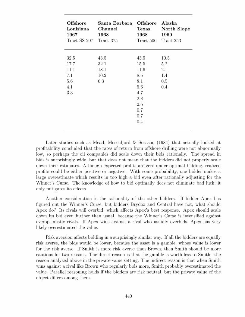
Offshore Santa Barbara Offshore AlaskaLouisiana Channel Texas North Slope1967 1968 1968 1969Tract SS 207 Tract 375 Tract 506 Tract 253

32.5 43.5 43.5 10.517.7 32.1 15.5 5.211.1 18.1 11.6 2.17.1 10.2 8.5 1.45.6 6.3 8.1 0.54.1 5.6 0.43.3 4.7

2.82.60.70.70.4

Later studies such as Mead, Moseidjord & Sorason (1984) that actually looked atprofitability concluded that the rates of return from offshore drilling were not abnormallylow, so perhaps the oil companies did scale down their bids rationally. The spread inbids is surprisingly wide, but that does not mean that the bidders did not properly scaledown their estimates. Although expected profits are zero under optimal bidding, realizedprofits could be either positive or negative. With some probability, one bidder makes alarge overestimate which results in too high a bid even after rationally adjusting for theWinner’s Curse. The knowledge of how to bid optimally does not eliminate bad luck; itonly mitigates its effects.

Another consideration is the rationality of the other bidders. If bidder Apex hasfigured out the Winner’s Curse, but bidders Brydox and Central have not, what shouldApex do? Its rivals will overbid, which affects Apex’s best response. Apex should scaledown its bid even further than usual, because the Winner’s Curse is intensified againstoveroptimistic rivals. If Apex wins against a rival who usually overbids, Apex has verylikely overestimated the value.

Risk aversion affects bidding in a surprisingly similar way. If all the bidders are equallyrisk averse, the bids would be lower, because the asset is a gamble, whose value is lowerfor the risk averse. If Smith is more risk averse than Brown, then Smith should be morecautious for two reasons. The direct reason is that the gamble is worth less to Smith– thereason analyzed above in the private-value setting. The indirect reason is that when Smithwins against a rival like Brown who regularly bids more, Smith probably overestimated thevalue. Parallel reasoning holds if the bidders are risk neutral, but the private value of theobject differs among them.

440

In fact, Capen, Clapp, and Campbell all worked for the oil company Arco, and devel-oped a bidding strategy for oil leases that took into account the Winner’s Curse. Companyexecutives realized that they were bidding too high, but were not clear about whether thesolution was to reduce the geological estimates, raise the discount rate, or something else,before the three worked out their strategy. There was debate within the company as towhether to make the idea of the Winner’s Curse public. The idea was a private advan-tage for Arco– but other oil company’s ignorance of it meant that they were bidding toohigh, which may have hurt them most, but hurt Arco too. After some years, the com-pany decided to let them reveal the secret (See “The Tale of the ’Winner’s Curse’ ” athttp://www.aapg.org/explorer/2004/12dec/capen.cfm)

The Winner’s Curse crops up in situations seemingly far removed from auctions. Anemployer should beware of hiring a worker passed over by other employers. Someonerenting an apartment should worry that he is the first potential renter who arrived when theneighboring trumpeter was asleep. A firm considering a new project should be concernedthat the project has been considered and rejected by competitors. The Winner’s Cursecan even be applied to political theory; certain proposals for innovations keep reappearingin the political arena over time. Will the first electorate to adopt them fall prey to theWinner’s Curse?

On the other hand, if information is revealed in the course of an auction, the fact thatvalues are common can lead to higher bidding, not lower. “Getting carried away” may be arational feature of a common-value auction. Suppose that the setting is not pure commonvalue, but a mix of a common value and private values. If a bidder has a high privatevalue and then learns in the course of the bidding that the common value is larger than hethought, he may well end up bidding more than he had planned and winning, but he wouldnot regret it afterwards. Especially in these mixed situations, when bidders have differentprivate values and when some but not all of each bidder’s information is revealed by hisbidding, common-value auctions can become very complicated indeed.

Strategies in Common-Value Auctions

Milgrom & Weber (1982) found that when there is a common-value element in anauction and signals are “affiliated” then revenue equivalence fails. The first-price anddescending auctions are still identical, but they raise less revenue than the ascending orsecond-price auctions. If there are more than two bidders, the ascending auction raisesmore revenue than the second-price auction. (In fact, if signals are affiliated then evenin a private value auction, in which each bidder knows his own value with certainty, thefirst-price and descending auctions will do worse.)

We will not prove the ranking of revenues by auction generally, but we will go throughan example with estimation errors that are uniformly distributed. This example will betractable because of some special properties of optimal estimates when errors are uniformlydistributed, so let’s start with discussion of those properties.

441

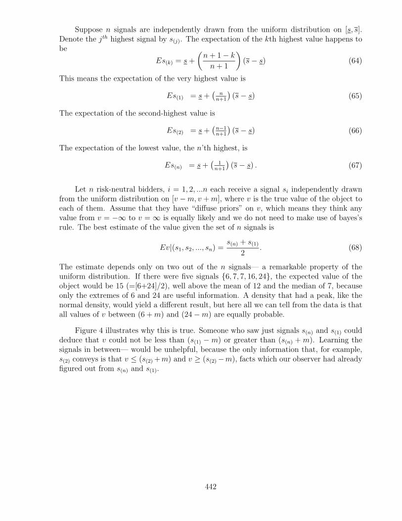
Suppose n signals are independently drawn from the uniform distribution on [s, s].Denote the jth highest signal by s(j). The expectation of the kth highest value happens tobe

Es(k) = s +

(n + 1− k

n + 1

)(s− s) (64)

This means the expectation of the very highest value is

Es(1) = s +(

nn+1

)(s− s) (65)

The expectation of the second-highest value is

Es(2) = s +(

n−1n+1

)(s− s) (66)

The expectation of the lowest value, the n’th highest, is

Es(n) = s +(

1n+1

)(s− s) . (67)

Let n risk-neutral bidders, i = 1, 2, ...n each receive a signal si independently drawnfrom the uniform distribution on [v −m, v + m], where v is the true value of the object toeach of them. Assume that they have “diffuse priors” on v, which means they think anyvalue from v = −∞ to v = ∞ is equally likely and we do not need to make use of bayes’srule. The best estimate of the value given the set of n signals is

Ev|(s1, s2, ..., sn) =s(n) + s(1)

2. (68)

The estimate depends only on two out of the n signals— a remarkable property of theuniform distribution. If there were five signals {6, 7, 7, 16, 24}, the expected value of theobject would be 15 (=[6+24]/2), well above the mean of 12 and the median of 7, becauseonly the extremes of 6 and 24 are useful information. A density that had a peak, like thenormal density, would yield a different result, but here all we can tell from the data is thatall values of v between (6 + m) and (24−m) are equally probable.

Figure 4 illustrates why this is true. Someone who saw just signals s(n) and s(1) coulddeduce that v could not be less than (s(1) −m) or greater than (s(n) + m). Learning thesignals in between— would be unhelpful, because the only information that, for example,s(2) conveys is that v ≤ (s(2) +m) and v ≥ (s(2)−m), facts which our observer had alreadyfigured out from s(n) and s(1).

442

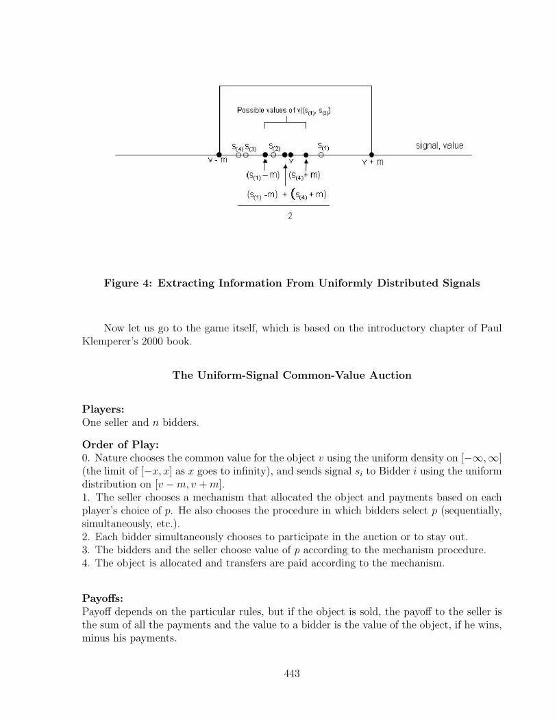
Figure 4: Extracting Information From Uniformly Distributed Signals

Now let us go to the game itself, which is based on the introductory chapter of PaulKlemperer’s 2000 book.

The Uniform-Signal Common-Value Auction

Players:One seller and n bidders.

Order of Play:0. Nature chooses the common value for the object v using the uniform density on [−∞,∞](the limit of [−x, x] as x goes to infinity), and sends signal si to Bidder i using the uniformdistribution on [v −m, v + m].1. The seller chooses a mechanism that allocated the object and payments based on eachplayer’s choice of p. He also chooses the procedure in which bidders select p (sequentially,simultaneously, etc.).2. Each bidder simultaneously chooses to participate in the auction or to stay out.3. The bidders and the seller choose value of p according to the mechanism procedure.4. The object is allocated and transfers are paid according to the mechanism.

Payoffs:Payoff depends on the particular rules, but if the object is sold, the payoff to the seller isthe sum of all the payments and the value to a bidder is the value of the object, if he wins,minus his payments.

443

What are the strategies in symmetric equilibria for the different auction rules? (we willignore possible asymmetric equilibria.)

The Ascending Auction (open-exit)

Equilibrium: If no bidder has quit yet, Bidder i should drop out when the price rises tosi. Otherwise, he should drop out when the price rises to pi =

p(n)+si

2, where p(n) is the

price at which the first dropout occurred.

Explanation: If no other bidder has quit yet, Bidder i is safe in agreeing to pay his signal,si. Either (a) he has the lowest signal, or (b) everybody else has the same signal value si

too, and they will all drop out at the same time. In case (a), having the lowest signal, hewill lose anyway. In case (b), the best estimate of the value is si, and that is where heshould drop out.

Once one bidder has dropped out at p(n), the other bidders can deduce that he had thelowest signal, so they know that signal s(n) must equal p(n). Suppose Bidder i has signalsi > s(n). Either (a) someone else has a higher signal and Bidder i will lose the auctionanyway and dropping out too early does not matter, or (b) everybody else who has not yetdropped out has signal si too, and they will all drop out at the same time, or (c) he wouldbe the last to drop out, so he will win. In cases (b) and (c), his estimate of the value is

p(i) =p(n)+si

2, since p(n) and si are the extreme signal values and the signals are uniformly

distributed, and that is where he should drop out.

The price paid by the winner will be the price at which the second-highest bidderdrops out, which is

s(n)+s(2)

2. The expected values are, from equations (66) and (67),

Es(n) = (v −m) +(

n+1−nn+1

)((v + m)− (v −m))

= v +(

1−nn+1

)m

(69)

andEs(2) = (v −m) +

(n+1−2

n+1

)((v + m)− (v −m))

= v +(

n−3n+1

)m.

(70)

Averaging them yields the expected winning price,

Ep(2) =[v+( 1−n

n+1)m]+[v+(n−3n+1)m]

2

= v −(

12

) (1

n+1

)2m.

(71)

If m = 50 and n = 4, then

Ep(2) = v −(

1

10

)(100) = v − 10. (72)

Expected seller revenue increases in n, the number of bidders (and thus of independentsignals) and falls in the uncertainty m (the inaccuracy of the signals). This will be true forall three auction rules we examine here.

444

It is not always true that the bidders can deduce the lowest signal in an ascendingauction and use that to form their bid. Their ability to discover s(n) depended crucially onthe open-exit feature of the auction— that the player with the lowest signal had to openlydrop out, rather than lurk quietly in the background. A secret-exit ascending auction wouldbehave like a second-price auction instead.

The Second-Price Auction

Equilibrium: Bid pi = si −(

n−2n

)m.

Explanation: In forming his strategy, Bidder i should think of himself as being tied forwinner with one other bidder, and so having to pay exactly his bid. Thus, he imagineshimself as the highest of (n−1) bidders drawn from [v−m, v +m] and tied with one other.On average, if this happens,

si = (v −m) +(

([n−1]+1−1)[n−1]+1

)([v + m]− [v −m])

= (v −m) +(

n−1n

)(2m)

= v +(

n−2n

)(m).

(73)

He will bid the value v which solves equation (73), yielding the optimal strategy, pi =si −

(n−2

n

)(m).

On average, the second-highest bidder actually has the signal Es(2) = v+(

n−3n+1

)m, from

equation (70). So the expected price, and hence the expected revenue from the auction, is

Ep(2) = [v +(

n−3n+1

)m]−

(n−2

n

)(m)

= v +(

n(n−3)−(n+1)(n−2)(n+1)n

)m,

= v −(

n−1n

) (1

n+1

)2m.

(74)

If m = 50 and n = 4, then

Ep(2) = v −(

3

4

)(1

5

)(100) = v − 15. (75)

If there are at least three bidders, expected revenue is lower in the second- priceauction. (We found revenue of (v − 10) with n = 4 in the ascending auction.) If n = 2,however, the expected price is the same in the second- price and ascending auctions. Then,v(n) = v(2), so the winning price is based on the same information in both auctions.

The First-Price Auction

Equilibrium: Bid (si −m).

445

Explanation: This is the simplest strategy of the three, but the hardest to derive. Bidderi bids (si − z) for some amount z that does not depend on his signal, because given theassumption of diffuse priors, he does not know whether his signal is a high one or a lowone. Define Ti to be how far the signal si is above its minimum possible value, (v−m), so

Ti ≡ si − (v −m) (76)

and si ≡ v−m+Ti. Bidder i has the highest signal and wins the auction if Ti is big enough,

which has probability(

Ti

2m

)n−1, which we will define as G(Ti), because it is the probability

that the (n − 1) other signals are all less than si = v −m + Ti. He earns v minus his bidof (si − z) if he wins, which equals (z + m− Ti).

If, instead, Bidder i deviated and bid a small amount ε higher, he would win with ahigher probability, G(Ti + ε), but he would lose ε whenever he would have won with thelower bid. Using a Taylor expansion, G(Ti + ε) ≈ G(Ti) + G′(Ti)ε, so

G(Ti + ε)−G(Ti) ≈ (n− 1)T n−2i

(1

2m

)n−1

ε. (77)

The benefit from bidding higher is the higher probability, [G(Ti + ε) − G(Ti)] times thewinning surplus (z +m−Ti). The loss from bidding higher is that the bidder would pay an

additional ε in the(

Ti

2m

)n−1cases in which he would have won anyway. In equilibrium, he

is indifferent about this infinitesimal deviation, taking the expectation across all possiblevalues of his “signal height” Ti, so∫ 2m

Ti=0

[((n− 1)T n−2

i

(1

2m

)n−1

ε

)(z + m− Ti)− ε

(Ti

2m

)n−1]

dTi = 0. (78)

This implies that

ε

(1

2m

)n−1 ∫ 2m

Ti=0

[((n− 1)T n−2

i

)(z + m)− (n− 1)T n−1

i − T n−1i

]dTi = 0. (79)

which in turn implies that

ε

(1

2m

)n−1 ∣∣∣∣2m

Ti=0

(T n−1

i (z + m)− T ni

)= 0, (80)

so (2m)n−1(z + m) − (2m)n − 0 + 0 = 0 and z = m. Bidder i’s optimal strategy in thesymmetric equilibrium is to bid pi = si −m.

446

The winning bid is set by the bidder with the highest signal, and that highest signal’sexpected value is

Es(1) = s +(

n+1−1n+1

)(s− s)

= v −m +(

nn+1

)((v + m)− (v −m))

= v −m +(

nn+1

)(2m)

(81)

The expected revenue is therefore

Ep(1) = v − (1)

(1

n + 1

)2m. (82)

If m = 50 and n = 4, then

Ep(1) = v −(

1

5

)(100) = v − 20. (83)

Here, the revenue is even lower than in the second-price auction, where it was (v−15) (andthe revenue is lower even if n = 2).

The revenue ranking is thus that the ascending open-exit auction has the highestexpected revenue for the seller, the second-price auction is in the middle, and the first-price auction is lowest. The revenue depends on how intensely bidders compete up theprice under each auction rule, which in turn depends on how much of an informationaladvantage the highest-signal-bidder has. In the ascending auction, all the bidders come toknow s(n), and the winning price and who wins depends on s(2) and s(1), so the bidder withthe highest signal has a relatively small advantage. In the second-price auction, the winningprice and who wins depends on s(2) and s(1), and that information comes to be known onlyto those two bidders. In the first-price auction, the winning price and who wins dependonly on s(1), so the bidder with the highest signal has the only relevant information. Thus,his informational rent is greatest under that auction rule. Paradoxically, the bidders preferan auction rule which makes it harder for them to pool their information and accuratelyestimate v. Or perhaps this is not paradoxical. What the seller would like best would befor every bidder to truthfully announce his signal publicly, because then every bidder wouldhave the same estimate, that would be the amount each would bid, and the informationalrent would fall to zero.

13.6 Asymmetric Equilibria, Affiliation, and Linkage: The Wallet Game

Asymmetric Equilibria in Common-Value Auctions

447

Besides the symmetric equilibria I have been discussing so far, asymmetric equilibriaare typical, robust, and plausible in common-value auctions. That is because the severityof the winner’s curse facing Bidder i depends on the bidding behavior of the other bidders.If other bidders bid aggressively, then if i wins anyway, he must have a big overestimate ofthe value of the object. So the more aggressive are the other bidders, the more conservativeought Bidder i to be— which in turn will make the other bidders more aggressive. TheWallet Game of Klemperer (1998) illustrates this.

The Wallet Game

PlayersSmith and Jones.

Order of Play(0) Nature chooses the amounts s1 and s2 of the money in each player’s wallet using densityfunctions f1(s1) and f2(s2). Each player observes only his own wallet’s contents.(1) Each player chooses a bid ceiling p1 or p2. An auctioneer auctions off the two walletsby gradually raising the price until either p1 or p2 is reached.

Payoffs:The player who bids less has a payoff of zero. The winning player pays the bid ceiling ofthe loser and hence has a payoff of

s1 + s2 −Min(p1, p2) (84)

A symmmetric equilibrium is for Bidder i to choose bid ceiling pi = 2si. This is anequilibrium because if he wins at exactly that price, Bidder j’s signal must be sj = si andthe value of the wallets is 2si. If Bidder i bids any lower, he might pass up a chance to buythe wallet for less than its value. If he bids any higher, he would only win if p > 2sj too,which implies that p > si + sj.

This equilibrium clearly illustrates how bidders should base their strategy on the strat-egy they expect the other bidders to use. Note that Bidder’s i’s strategy is unrelated tohis prior beliefs about Bidder j’s value. It might be, for example, that using f2(s2), theexpected value of s2 is 100, but if Bidder 1’s wallet contains s1 = 8, he should just bid 16.So doing, he will probably lose, but if he bids 108 and wins, it will only be because Bidder2’s wallet contains 54 or less. That is fine if it contains 8 or less, but if it contains, forexample, s2 = 9, then Bidder 2 will bid up to 18 and stop, Bidder 1 will win with his bidceiling of 108, and his payoff will be 8 + 9− 18 = −1.

The Wallet Game has both independent values and pure common values, a curiouscombination. The value of the two wallets is the same for both bidders, but the signaleach receives is independent. Knowing s1 is useless in predicting s2, though it is useful inpredicting the common value.

448

The independence of the signals makes a bidder’s optimal strategy particularly sensi-tive to what he thinks the other bidder’s strategy is, since his own signal tells him noth-ing about the other player’s signal and he must rely on the other player’s bidding forany information about it. Thus, there are many asymmetric equilibria. One of them is(p1 = 10s1, p2 = 10

9s2). If the two players tie, having choosen p = p1 = p2, then 10s1 = 10

9s2,

which implies that s1 = 19s2, so s1 + s2 = 10s1 = p, and v = p. This is a bad equilibrium

for Bidder 2 because he hardly ever wins and when he does win it’s because s1 was verylow— so there is hardly any money in Bidder 1’s wallet. Being the aggressive bidder inan equilibrium is valuable. If there is a sequence of auctions, this means establishing areputation for aggressiveness can be worthwhile, as shown in Bikhchandani (1988).

Asymmetric equilibria can even arise when the players are identical. Second- price,two-person, common-value auctions usually have many asymmetric equilibria besides thesymmetric equilibrium we have been discussing (see Milgrom [1981c] and Bikhchandani[1988]). Suppose that Smith and Brown have identical payoff functions, but Smith thinksBrown is going to bid aggressively. The winner’s curse is intensified for Smith, who wouldprobably have overestimated if he won against an aggressive bidder like Brown, so Smithbids more cautiously. But if Smith bids cautiously, Brown is safe in bidding aggressively,and there is an asymmetric equilibrium. For this reason, acquiring a reputation for aggres-siveness is valuable.

Oddly enough, if there are three or more bidders the second-price, common- valueauction has a unique equilibrium, which is also symmetric. The open-exit ascending auctionis different: it has asymmetric equilibria, because after one bidder drops out, the tworemaining bidders know that they are alone together in a subgame which is a two-bidderauction. Regardless of the number of bidders, first-price auctions do not have this kind ofasymmetric equilibrium. Threats in a first-price auction are costly because the high bidderpays his bid even if his rival decides to bid less in response. Thus, a bidder’s aggressivenessis not made safer by intimidation of another bidder.

Affiliation, the Monotone Likelihood-Ratio Property, and the Linkage Princi-ple6

Milgrom & Weber (1982) introduced the idea of affiliation: a formal definition of twovariables tending to move upwards together that is useful in the auction context. Supposebidder 1 has a value v1 which is a increasing function of a private signal x1 that he receives,and which might also depend on the private signal of bidder 2, x2. What we need to knowto analyze the auction is what happens to bidder 1’s estimate of his value as he observesor deduces more about bidder 2’s signal. A simple and plausible situation is that wheneverhe learns that x2 takes a large value, his estimate of his value v1 rises. Thus, if he observesbidder 2 bid more and he deduces that x2 is large, he should increase his estimate of v1.Affiliation is defined so this will happen if the signals x1 and x2 are strongly affiliated, andif they are weakly affiliated, bidder 1’s estimate of v1 at least will not fall as x2 rises. Forsimplicity, I will define affiliation for the case of two signals.

6Much of this discussion is based on Cramton (undated), Klemperer (2004, p. 51) and Wolfstetter(1999).

449

Definition. The signals x1 and x2 are affiliated if for all possible realizations Small < Bigof x1 and Low < High of x2, the joint probability f(x1, x2) is such that z1 and z2,

f(x1 = Small, x2 = Low)f(x1 = Big, x2 = High) ≥ f(x1 = Small, x2 = High)f(x1 = Big, x2 = Low).(85)

Thus, affiliation says that the probability the values of x1 and x2 move in the same direc-tion is greater than the probability they move oppositely. Notice that this allows a jointprobability distribution such as the following, in which even if x2 is Low, x1 is probablyBig.

Prob(x1 = Big, x2 = High) = 0.5Prob(x1 = Small, x2 = Low) = 0.1Prob(x1 = Big, x2 = Low) = 0.2Prob(x1 = Small, x2 = High) = 0.2

Imagine that Bidder 3, who is ignorant of both x1 and x2, can deduce about x1 if helearns that x2 = Low. Bidder 3’s prior is

Prob(x1 = Big) = Prob(x1 = Big, x2 = High) + Prob(x1 = Big, x2 = Low)

= 0.5 + 0.2 = 0.7.(86)

Suppose Bidder 3 finds out that x2 is Low. We will use the same kind of manipulationas in bayes’s rule, though not bayes’s rule itself. Since

Prob(x1 = Big, x2 = Low) = Prob(x1 = Bigh|x2 = Low)Prob(x2 = Low), (87)

we can write Bidder 3’s posterior as

Prob(x1 = Big|x2 = Low) = Prob(x1=Big,x2=Low)Prob(x2=Low)

= 0.2Prob(x1=Big,x2=Low)+Prob(x1=Small,x2=Low)

= 0.20.2+0.1

(88)

Thus, observing x2 = Low leaves Bidder 3 still thinking that probably x1 = Big, but theprobability has fallen from 0.7 to 0.66. x2 = Low is bad news about the value of x1.

The big implication of two signals being affiliated is that the expected value of thewinning bid conditional on the signals is increasing in all the signals. When one signalrises, that has the positive direct effect of increasing the bid of the player who sees it, andnon-negative indirect effects once the other players see his bid increase and deduce that hehad a high signal.

This is very much like the Monotone Likelihood-Ratio Property, which is the samething expressed in terms of the conditional densities, the posteriors.

450

Definition. The conditional probability g(x1|x2) satisfies the Monotone Likelihood RatioProperty if the likelihood ratio is weakly decreasing in x1, that is, for all possible realizationsSmall < Big of x1 and Low < High of x2,

g(Big|Low)

g(Big|High)≤ g(Small|Low)

g(Small|High). (89)

The Monotone Likelihood Ratio Property says that as x2 goes from Low to High, theBig value of x1 becomes relatively more likely. It can be shown that this implies that forany value z, the conditional cumulative distribution of x1 up to x1 = z given x2 weaklyincreases with x2, which is to say that the distribution G(x1|x2) conditional on a largervalue of x2 stochastically dominates the distribution conditional on a smaller value of x2.

This no doubt leaves the reader’s head spinning quite as much as it does the author’s,despite my attempt at simplification. A final, equivalent definition of affiliation, applicablewhen the signals are distributed according to a joint density f(x1, x2) that is continuousand twice differentiable is that x1 and x2 are affiliated if

∂log(f)2

∂x1∂x2

≥ 0. (90)

One of the rewards of establishing that bidders’ signals are affiliated is the linkageprinciple, which says that when the amount of affiliated information available to biddersincreases, the equilibrium sales price becomes greater. Thus, the seller should have apolicy of disclosing any affiliated information he possesses. Also, auction rules which revealaffiliated information in the course of the auction (e.g., open-exit auctions) or use it indetermining the winner’s payment (e.g., the second-price auction) will result in higherprices. We saw this in the Uniform-Signal Common-Value Auction examples. The resultis not restricted to common-value auctions, however; seller revenue rises when affiliatedinformation is released even in an affiliated private value auction, in which the bidders eachknow their own private values but not those of other bidders. The intuition behind thelinkage principle is hard to grasp, because it applies even when there is no winner’s curse(as in the affiliated private value auction), and it does not always apply in common valueauctions (when there are just two bidders, the ascending auction is not superior to thesecond-price auction, as we saw above). The best intuition I have seen is that on page 128of Klemperer (2004): that bidder profits arise from their private information, and releaseof affiliated information reveals something about the private information of each bidder,including, especially, the one who will win, and thus heightens competition.

The linkage principle provides a reason why sellers may wish to extend auctions overtime in multiple rounds, why they should encourage active bidding throughout rather thanlet bidders “lurk” and suddenly bid near the end, why they should lay out their owninformation as clearly and early as possible, and why they should let bidders know eachothers’ identities. The idea is a slippery one, howevever, and Perry & Reny (1999) showthat the linkage principle actually can fail if more than one unit of the good is beingauctioned, so players submit bids for the possible purchase of multiple units. Multiple-unitauctions and “package auctions,” in which not just multiple units but multiple objects aresold in a single auction, are active areas of research.

451

Notes

N13.1 Values Private and Common, Continuous and Discrete

• Milgrom & Weber (1982) is a classic article that covers many aspects of auctions. McAfee& McMillan (1987) is an excellent older survey of auction theory which takes some pains torelate it to models of asymmetric information. More recent is Maskin (2004). Klemperer(2000) collects many of the most important articles in an edited volume. Vijay Krishna’s2002 Auction Theory, Paul Klemperer’s 2004 Auctions: Theory and Practice (which isrelatively nontechnical), and Paul Milgrom’s 2004 Putting Auction Theory to Work (whichis very good on the mathematical assumptions) are good textbook treatments. I particularlylike the auction chapters in Elmar Wolfstetter’s 1999 Topics in Microeconomics: IndustrialOrganization, Auctions, and Incentives. Paul Milgrom’s consulting firm, Agora MarketDesign, has a website with many good working papers that can be found via http:www.market-design.com.

• Cassady (1967) is an excellent source of pre-Web institutional detail. The appendix to hisbook includes advertisements and sets of auction rules, and he cites numerous newspaperarticles. The rise of the Web, an ideal setting for auctions, fortuitously occurred at thesame time as the rise of auction theory. See Bajari & Hortacsu’s 2004 survey, “EconomicInsights from Internet Auctions.”

N13.2 Optimal Strategies under Different Rules in Private-Value Auctions

• Many (all?) leading auction theorists were involved in the seven-billion dollar spectrumauction by the United States government in 1994, either helping the government choosean auction rule to sell spectrum or helping bidders decide how to buy it. Paul Milgrom’s1999 book, Auction Theory for Privatization, tells the story. See also McAfee & McMillan(1996). Interesting institutional details have come in the spectrum auctions and stimulatednew theoretical research. Ayres & Cramton (1996), for example, explore the possibility thataffirmative action provisions designed to help certain groups of bidders may have actuallyincreased the revenue raised by the seller by increasing the amount of competition in theauction.

• One might think that an ascending second-price, open-cry auction would come to the sameresults as an ascending first-price, open-cry auction, because if the price advances by ε ateach bid, the first and second bids are practically the same. But the second-price auctioncan be manipulated. If somebody initially bids $10 for something worth $80, another biddercould safely bid $1,000. No one else would bid more, and he would pay only the secondprice: $10.

• Auctions are especially suitable for empirical study because they are so stylized and generatemasses of data. Hendricks & Porter (1988) is a classic comparison of auction theory withdata. See Bajari, Hong & Ryan (2004) or the Athey & Haile (2005) and Hendricks & Porter(forthcoming) surveys of empirical work on auctions.

• After the last bid of an open-cry art auction in France, the representative of the Louvrehas the right to raise his hand and shout “pre- emption de l’etat,” after which he takes thepainting at the highest price bid (The Economist, May 23, 1987, p. 98). How does thataffect the equilibrium strategies? What would happen if the Louvre could resell?

452

• Share Auctions. In a share auction each bidder submits a bid for both a quantity anda price. The bidder with the highest price receives the quantity for which he bid at thatprice. If any of the product being auctioned remains, the bidder with the second-highestprice takes the quantity he bid for, and so forth. The rules of a share auction can alloweach bidder to submit several bids, often called a schedule of bids. The details of shareauctions vary, and they can be either first-price or second-price. Modelling is complicated;see Wilson (1979).

N13.3 Revenue Equivalence, Risk Aversion, and Uncertainty

• Che & Gale (1998) point out that if bidders differ in their willingness to pay in a privatevalue auction because of budget constraints rather than tastes then the revenue equivalencetheorem can fail. The following example from page 2 of their paper shows this. Supposetwo budget-constrained bidders are bidding for one object. In Auction 1, each bidder has abudget of 2 and knows only his own value, which is drawn uniformly from [0,1]. The budgetconstraints are never binding, and it turns out that the expected price is 1/3 under eithera first-price or a second-price auction. In Auction 2, however, each bidder knows only hisown budget, which is drawn uniformly from [0,1], and both have values for the object of 2.The budget constraint is always binding, and the equilibrium strategy is to bid one’s entirebudget under either set of auction rules. The expected price is still 1/3 in the second- priceauction, but now it is 2/3 in the first-price auction. The seller therefore prefers to use afirst-price auction.

• A Mechanism To Extract All the Surplus. Myerson (1981) shows that if thebidders’ private information is correlated, the seller can construct something akin to aMaskin matching scheme mechanism of the kind discussed in Chapter 10 that extracts allthe information and all the surplus. In the Uniform-Signal Common-Value Auction, wheresignals are uniform in [v −m, v + m] ask Bidder i to bid si, allocate the good to the highbidder at the price s(1)+s(n)

2 , which is an unbiased estimate of v, and ensure truthtellingby the boiling-in-oil punishment of a large negative payment if the reports are such thats(n) < s(1) −m, which cannot possibly occur if all bidders tell the truth.

453

N13.4 Common-Value Auctions and the Winner’s Curse

Rothkopf (1969) and Wilson (1969) seem to the be first published accounts of the Winner’sCurse. An article on Edward Capen, “The Tale of the ’Winner’s Curse’ ” at http://www.aapg.org/explorer/2004/12dec/capen.cfmsays that the term was first published in Capen, Clapp & Campbell (1971). I recommendthe article for its tale of the use of theory in business practice.

• The Winner’s Curse and the idea of common values versus private values have broad appli-cation. The Winner’s Curse is related to the idea of “regression to the mean” discussed inSection 2.4 of this book. Kaplow & Shavell (1996) use the idea to discuss property versusliability rules, one of the standard rule choices in law-and-economics. If someone violatesa property rule, the aggrieved party can undo the violation, as when a thief is required tosurrender stolen property. If someone violates a liability rule, the aggrieved party can onlyget monetary compensation, as when someone who breaches a contract is required to paydamages to the aggrieved party. Kaplow and Shavell argue that if a good has independentvalues, a liability rule is best because it gives efficient incentives for rule violation; but if ithas common value and courts make errors in measuring the common value, a property rulemay be better. See especially page 761 of their article.

N13.6 Asymmetric Equilibria, Affiliation, and Linkage: The Wallet Game

• Even if value estimates are correlated, the optimal bidding strategies can still be the sameas in private-value auctions if the values are independent. If everyone overestimates theirvalues by 10 percent, a bidder can still extract no information about his value by seeingother bidders’ value estimates.

454

Problems

13.1. Rent Seeking (medium)Two risk-neutral neighbors in sixteenth century England, Smith and Jones, have gone to courtand are considering bribing a judge. Each of them makes a gift, and the one whose gift is thelargest is awarded property worth £2,000. If both bribe the same amount, the chances are 50percent for each of them to win the lawsuit. Gifts must be either £0, £900, or £2,000.

(a) What is the unique pure-strategy equilibrium for this game?

(b) Suppose that it is also possible to give a £1500 gift. Why does there no longer exist apure-strategy equilibrium?

(c) What is the symmetric mixed-strategy equilibrium for the expanded game? What is thejudge’s expected payoff?

(d) In the expanded game, if the losing litigant gets back his gift, what are the two equilibria?Would the judge prefer this rule?

13.2. The Founding of Hong Kong (medium)The Tai-Pan and Mr. Brock are bidding in an ascending auction for a parcel of land on a knollin Hong Kong. They must bid integer values, and the Tai-Pan bids first. Tying bids cannot bemade, and bids cannot be withdrawn once they are made. The direct value of the land is 1 toBrock and 2 to the Tai-Pan, but the Tai-Pan has said publicly that he wants it, so if Brock gets it,he receives 5 in “face” and the Tai-Pan loses 10. Moreover, Brock hates the Tai-Pan and receives1 in utility for each 1 that the Tai-Pan pays out to get the land.

(a) First suppose there were no “face” or “hate” considerations, just the direct values. Whatare the equilibria if the Tai-pan bids first?

(b) Continue supposing there were no “face” or “hate” considerations, just the direct values.What are the three possible equilibria if Mr. Brock bids first? (Hint: in one of them, Brockwins; in the other two, the Tai-pan wins.)

(c) Fill in the entries in Table 2, including the “face” and “hate” considerations.

Table 2: The Tai-Pan Game

455

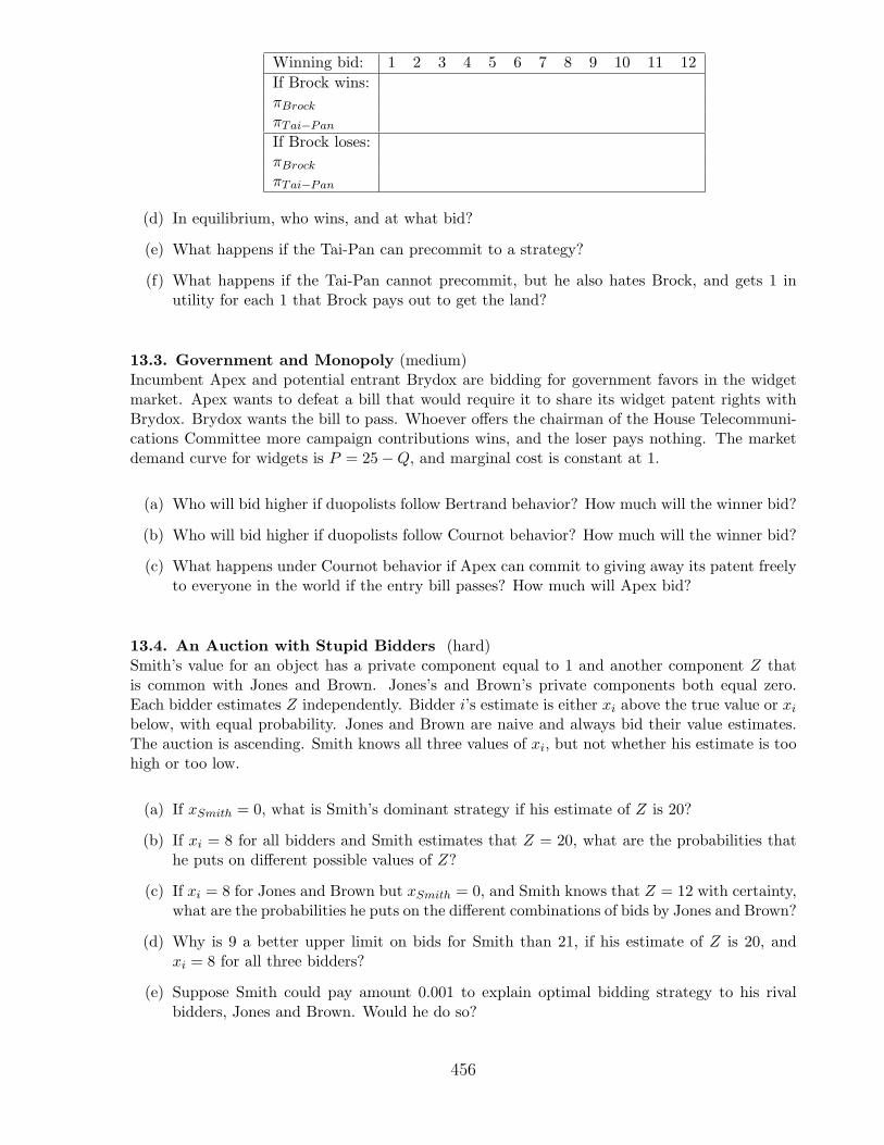
Winning bid: 1 2 3 4 5 6 7 8 9 10 11 12If Brock wins:πBrock

πTai−Pan

If Brock loses:πBrock

πTai−Pan

(d) In equilibrium, who wins, and at what bid?

(e) What happens if the Tai-Pan can precommit to a strategy?

(f) What happens if the Tai-Pan cannot precommit, but he also hates Brock, and gets 1 inutility for each 1 that Brock pays out to get the land?

13.3. Government and Monopoly (medium)Incumbent Apex and potential entrant Brydox are bidding for government favors in the widgetmarket. Apex wants to defeat a bill that would require it to share its widget patent rights withBrydox. Brydox wants the bill to pass. Whoever offers the chairman of the House Telecommuni-cations Committee more campaign contributions wins, and the loser pays nothing. The marketdemand curve for widgets is P = 25−Q, and marginal cost is constant at 1.

(a) Who will bid higher if duopolists follow Bertrand behavior? How much will the winner bid?

(b) Who will bid higher if duopolists follow Cournot behavior? How much will the winner bid?

(c) What happens under Cournot behavior if Apex can commit to giving away its patent freelyto everyone in the world if the entry bill passes? How much will Apex bid?

13.4. An Auction with Stupid Bidders (hard)Smith’s value for an object has a private component equal to 1 and another component Z thatis common with Jones and Brown. Jones’s and Brown’s private components both equal zero.Each bidder estimates Z independently. Bidder i’s estimate is either xi above the true value or xi

below, with equal probability. Jones and Brown are naive and always bid their value estimates.The auction is ascending. Smith knows all three values of xi, but not whether his estimate is toohigh or too low.

(a) If xSmith = 0, what is Smith’s dominant strategy if his estimate of Z is 20?

(b) If xi = 8 for all bidders and Smith estimates that Z = 20, what are the probabilities thathe puts on different possible values of Z?

(c) If xi = 8 for Jones and Brown but xSmith = 0, and Smith knows that Z = 12 with certainty,what are the probabilities he puts on the different combinations of bids by Jones and Brown?

(d) Why is 9 a better upper limit on bids for Smith than 21, if his estimate of Z is 20, andxi = 8 for all three bidders?

(e) Suppose Smith could pay amount 0.001 to explain optimal bidding strategy to his rivalbidders, Jones and Brown. Would he do so?

456

13.5. A Teapot Auction with Incomplete Information (easy)Smith believes that Brown’s value vb for a teapot being sold at auction is 0 or 100 with equalprobability. Smith’s value of vs = 400 is known by both bidders.

(a) What are the bidders’ equilibrium strategies in an open cry auction? You may assume thatin case of ties, Smith wins the auction.

(b) What are the bidders’ equilibrium strategies in a first-price sealed-bid auction? You mayassume that in case of ties, Smith wins the auction.

(c) Now let vs = 102 instead of 400. Will Smith use a pure strategy? Will Brown? You neednot find the exact strategies used.

457

Auctions: A Classroom Game for Chapter 13

The instructor will bring to class a glass jar of pennies to be auctioned off. There are between0 and 100 pennies in the jar, the number being drawn from a uniform distribution. Twenty percentof the students in the class must close their eyes while the jar is being displayed. The instructorwill pass the jar around to the other students in the class to let them try to figure out how manypennies are inside. He will then auction off the jar five times, using five different sets of rules.(The instructor will decide for himself whether to play for real money or not.)

The first auction will be a first-price auction. Each student submits a bid, and also recordhis estimate of the number of pennies.

The second auction will be a second-price auction. Each student submits a bid, and alsorecord his estimate of the number of pennies.

The third auction will be an all-pay auction. Each student submits a bid, and also recordhis estimate of the number of pennies.

The fourth auction will be a descending auction. After the auction, each student submitshis estimate of the number of pennies.

The fifth auction will be an ascending auction. After the auction, each student submits hisestimate of the number of pennies.

At this point, the instructor will announce the number of pennies in the jar, and the resultsof each auction.

458