1

Paper 123-2012

Trend Analysis: An Automated Data Quality Approach for Large Health Administrative Databases

Mahmoud Azimaee, Institute for Clinical Evaluative Sciences (ICES), Toronto, ON, Canada

ABSTRACT

Stability across time is one of the important components in Data Quality Assurance Process. This paper talks about a SAS® macro that has been designed to automate testing of stability across time as part of a larger data quality application package. Outlier analysis has been used for identifying unusual changes over time within large health administrative databases. The macro chooses the most appropriate model for smoothing the data curve/line. Potential outliers will be flagged on the scatterplot as suspicious points. Results will be presented only in a graphic format to be included in a Data Quality Report.

INTRODUCTION

The Manitoba Center for Health Policy (MCHP), a research unit within the Faculty of Medicine, University of Manitoba, has a data repository that includes over 65 health and other administrative databases, which are all linkable using a common encrypted individual identifier. MCHP receives annual updates for most of the databases in this collection. In July 2010 the author was asked to work on designing and implementing a Data Quality Process for MCHP’s Data Management Unit. Considering the growing number of databases and overall volume of data in the Repository, it was clear that any process had to work with the minimum amount of manual activity. Therefore, automation was an important factor in this process. After studying different data quality frameworks from similar data holding organization in Canada

[3, 5, 7], the UK

[8] and Australia

[1, 2], a specific data quality framework for MCHP was

designed. A package of 17 SAS macros was designed to apply this framework to the data in the MCHP repository. The MCHP’s Data Quality Framework consists of 5 major dimensions which are: Accuracy, Internal Validity, External Validity, Timeliness and Interpretability. Each dimension has its own components such as Completeness and Correctness. This paper will introduce a method and a SAS macro to evaluate Stability Across Time which is one of the components of the second dimension, Internal Validity.

STABILITY ACROSS TIME

According to the Canadian Institute for Health Information (CIHI)’s Data Quality Framework, stability across time is one of most important data quality indicators for health administrative databases.

The CIHI Data Quality Framework indicates [3]

:

Trend analysis is used to examine changes in core data elements over time

Changes in methodology or inclusion/exclusion criteria should be taken into account to determine whether the observed changes were real or not

Trend analysis includes comparisons of counts or proportions over time, as well as more sophisticated time series analysis, smoothing or curve fitting.

Graphing data is usually particularly helpful for investigating temporal changes.

When data is expected to naturally trend upward or downward due to policies implemented or social or economic changes, no change across years may also be an indication of a problem

METHOD

Considering CIHI’s guidelines [3]

, outlier analysis was chosen to identify unusual changes over time. To perform an

outlier analysis, the first step is to choose the best model that fits the data and the second step is to find the outliers

based on the selected model. In statistical methods it is usually recommended to use a scatterplot to investigate the

observations’ behavior. However, in order to automate the process and reduce the manual investigations, it is

necessary to find the most appropriate model for smoothing data. To achieve this goal, a set of seven common

models which are appropriate for health administrative data were selected:

Data ManagementSAS Global Forum 2012

Trend Analysis: An Automated Data Quality Approach for Large Health Administrative Databases, continued

2

1. Simple Linear: Y=β0 + β1X

2. Quadratic: Y= β0 + β1X2

3. Exponential: Y= β0 + β1exp(X)

4. Logarithmic: Y= β0 + β1log(X)

5. SQRT: Y= β0 + β1√

6. Inverse: Y= β0 + β1

7. Negative Exponential: Y= β0 + β1Exp(-X)

The models were fitted to the aggregated observations over fiscal years or months (using a date variable coded as 1,

2, 3…). For each model, the root mean square error (RMSE) between the model’s output and observations was

calculated; and the model with minimum RMSE was selected as the optimum model to represent the observations.

Secondly, the chosen model was re-fitted to the data to perform an outlier analysis and to calculate studentized

residuals without current observation. For each observation (fiscal years or months) this statistic was compared with

the t distribution (.95, n-p-1), where n is the number of fiscal years (or months) and p is the number of estimated

parameters (which is always equal to 2 in this analysis.). Significant observations were considered as potential

outliers or data quality problems. These steps were implemented in a SAS macro that flags observations based on

the following rules:

1. Observations with absolute Studentized Residuals greater than +/- t(.95, n-p-1) are flagged as potential outliers.

2. Since no variation over time may be an indication of a problem, the Macro also flags subsequent identical subsequent observations.

3. The macro also checks for small absolute annual number of records (between 1 and 5 inclusive). Majority of Canadian Health research organizations that use administrative data have a privacy policy which requires that no value based on six or fewer observations can be reported. If the Macro finds any cell frequencies of less than six, it replaces them with 3 (the average of all possible small numbers as an estimated value). It is important to notice that modeling and outlier analysis are done based on the actual numbers; but for demonstration of the trend graphs, small numbers are changed to 3 to comply with the privacy policy. (Any publication or presentation of material must represent more than 5 individuals or events

[6])

4. Trend graphs along with the fitted model are generated by the SAS Macro. In the trend graphs, potential outliers, identical subsequent observations and suppressed values are shown in red, orange and green, respectively.

MACRO’S SYNTAX AND PARAMETERS

Syntax: %TREND (DS =, STARTYR =, ENDYR =, BYDATE =, BYVAR =, BYFMT =, PATH = );

Description: For a given dataset, this Macro performs a trend over a specified time range. The results will be only in graphic formats.

Parameters: DS: Name of Dataset STARTYR: Beginning fiscal year (1st part, 4-digit) ENDYR: Ending fiscal year (1st part, 4-digit) BYDATE: Desired Date variable (Must be SAS Date) BYVAR: An optional categorical variable. If omitted only one trend analysis will be done for all the records in the table. BYFMT: An optional Format for BYVAR if there exists any. BYMONTH: Assign value of YES to this optional parameter to force analysis by month instead of fiscal year (default value is NO means fiscal year) PATH: A full path location for saving graphs in PNG format (must be in a double quotation mark)

Data ManagementSAS Global Forum 2012

Trend Analysis: An Automated Data Quality Approach for Large Health Administrative Databases, continued

3

Examples: %TREND (DS = health.med_2003mar, STARTYR = 2003, ENDYR = 2010, BYDATE = admit_dt, BYVAR = HOSP, PATH = “C:\DQ\”); %TREND (DS=health.virustests_19922010, STARTYR=1992, ENDYR=2009, BYDATE=RECEIVEDDT, PATH = “C:\DQ\”); %TREND (DS=health.virustests_19922010, STARTYR=1992, ENDYR=2009, BYDATE=RECEIVEDDT, BYFMT=$HOSPFMTL., PATH = “C:\DQ\”); %TREND (DS=health. virustests_19922010, STARTYR=1992, ENDYR=2009, BYDATE=RECEIVEDDT, MONTHLY=YES, PATH = “C:\DQ\”);

HOW DOES THE MACRO WORK?

The Trend Macro works with three other intermediate macros: GETNOBS, FISCALYR and MONTHLY. These

intermediate macros will be invoked by the TREND Macro and therefore, they must be available; however, the user

does not need to use them directly. GETNOBS returns number of observations in a given dataset; two other macros

create an appropriate fiscal year or monthly format for the given range in STARTYR and ENDYR.

%MACRO GETNOBS(DS) ;

%GLOBAL NO; %LET NO=; data _null_; if 0 then set &DS nobs=nobs;

call symput('NO',nobs); stop; run; %MEND GETNOBS;

Code box 1- GETNOBS Macro, an intermediate macro to return number of observation for a given dataset.

Depending on the user’s choice, all the analyses will be based on fiscal year or month, within the requested range.

Then using PROC FREQ, data are aggregated over the time variable, and optionally over another categorical

variable (as a BY Variable, e.g. by hospitals). Then, the required explanatory variables for each of the seven

mentioned models are created. The first PROC REG runs all the models against the summarized data and generates

RMSE using EDF option:

Data ManagementSAS Global Forum 2012

Trend Analysis: An Automated Data Quality Approach for Large Health Administrative Databases, continued

4

%Macro FISCALYR(startyr,endyr);

data fiscalyr; fmtname ='fy'; startChar='01Apr'; middle='31Mar'; startnum=SYMGETN('startyr'); endnum=SYMGETN('endyr'); yrs=endnum - startnum; do i=0 to yrs;

lcl=startnum + i; ucl=lcl + 1;

valueChar=startChar || put(lcl,$4.); ENDChar= middle || put(ucl,$4.); Start=input(valueChar,date9.); End=input(endChar,date9.); LABEL= compress(put(lcl,$4.) || "/" || substr(put(ucl,$4.),3,2));

output; end; run; data fiscalyr; length label $ 11 ;

set fiscalyr end=eof; output; if eof then do; HLO='O'; label='Other Years'; start=0; end=0;

output; end; keep fmtname start end label HLO; run; proc format cntlin=fiscalyr; run; proc datasets library=work ; delete fiscalyr; run; quit; %Mend FISCALYR;

Code box 2- FISCALYR Macro, an intermediate macro to create a format for fiscal years within the given range.

proc reg data=trend_data outest=parms noprint;

Linear: model COUNT=Time / EDF ;

Quatratic: model COUNT=Time2 / EDF ;

Exponential: model COUNT=exptime / EDF ;

Logaritmic: model COUNT=logtime / EDF ;

SQRT: model COUNT=sqrttime / EDF ;

Inverse: model COUNT=inverstime / EDF ;

Neg_Exponential: model COUNT=negexptime / EDF ;

by trend_by;

run;

Code box 3- Initial Regression Models.

Data ManagementSAS Global Forum 2012

Trend Analysis: An Automated Data Quality Approach for Large Health Administrative Databases, continued

5

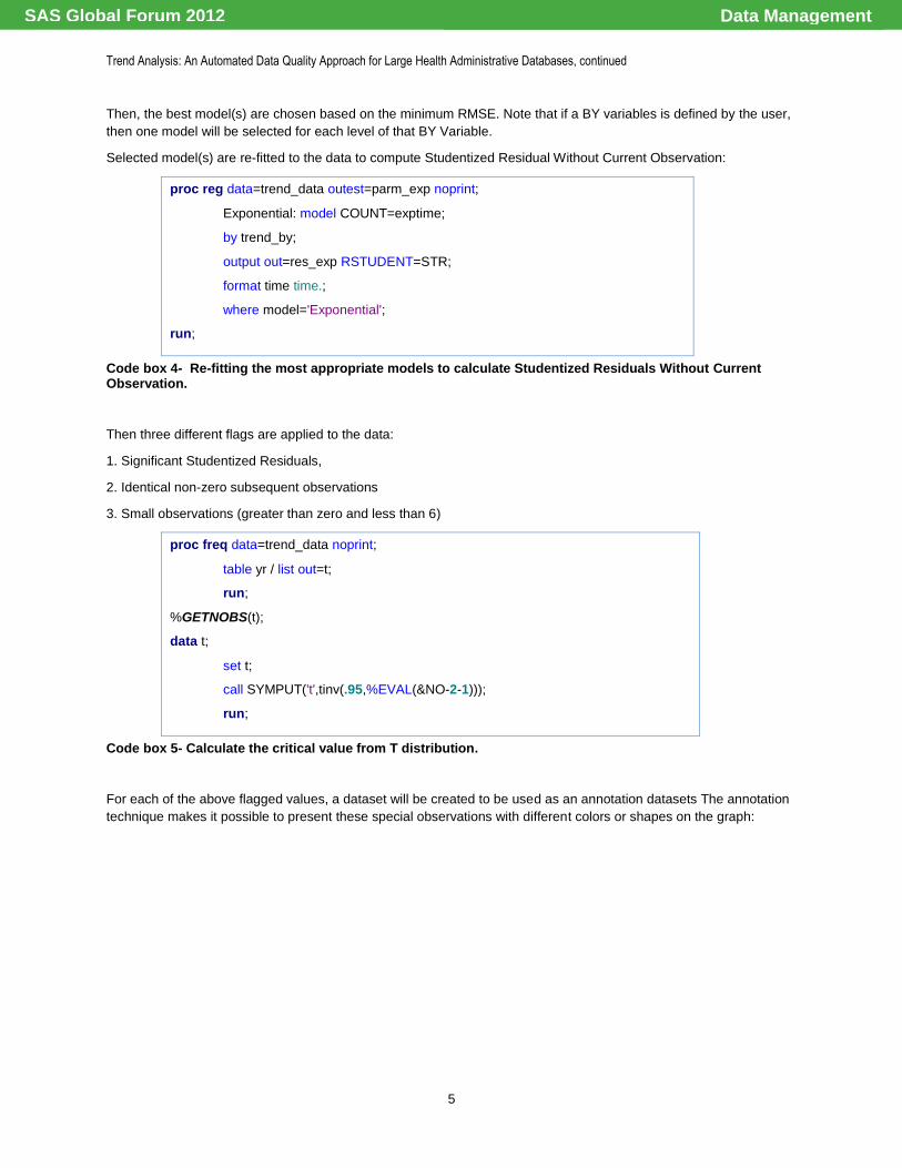
Then, the best model(s) are chosen based on the minimum RMSE. Note that if a BY variables is defined by the user,

then one model will be selected for each level of that BY Variable.

Selected model(s) are re-fitted to the data to compute Studentized Residual Without Current Observation:

proc reg data=trend_data outest=parm_exp noprint;

Exponential: model COUNT=exptime;

by trend_by;

output out=res_exp RSTUDENT=STR;

format time time.;

where model='Exponential';

run;

Code box 4- Re-fitting the most appropriate models to calculate Studentized Residuals Without Current Observation.

Then three different flags are applied to the data:

1. Significant Studentized Residuals,

2. Identical non-zero subsequent observations

3. Small observations (greater than zero and less than 6)

proc freq data=trend_data noprint;

table yr / list out=t;

run;

%GETNOBS(t);

data t;

set t;

call SYMPUT('t',tinv(.95,%EVAL(&NO-2-1)));

run;

Code box 5- Calculate the critical value from T distribution.

For each of the above flagged values, a dataset will be created to be used as an annotation datasets The annotation

technique makes it possible to present these special observations with different colors or shapes on the graph:

Data ManagementSAS Global Forum 2012

Trend Analysis: An Automated Data Quality Approach for Large Health Administrative Databases, continued

6

data graphlabel(keep=function xsys ysys xc y text color position size trend_by

trend_by2);

set trend_data;

by trend_by2;

* Define annotate variable attributes;

length color function $8 text $30;

retain function 'symbol'

xsys ysys '2'

color 'red'

position '2'

size 1.8;

if outlier=1 then do;

* Create a label;

text = 'dot';

%IF &BYMONTH=NO %THEN xc=yr;;

%IF &BYMONTH=YES %THEN xc=monthyr;;

y=count;

output graphlabel;

end;

run;

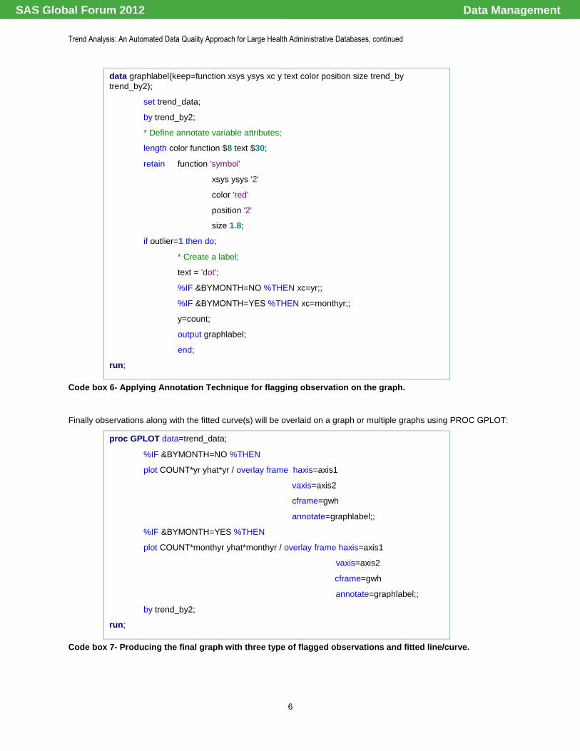
Code box 6- Applying Annotation Technique for flagging observation on the graph.

Finally observations along with the fitted curve(s) will be overlaid on a graph or multiple graphs using PROC GPLOT:

proc GPLOT data=trend_data;

%IF &BYMONTH=NO %THEN

plot COUNT*yr yhat*yr / overlay frame haxis=axis1

vaxis=axis2

cframe=gwh

annotate=graphlabel;;

%IF &BYMONTH=YES %THEN

plot COUNT*monthyr yhat*monthyr / overlay frame haxis=axis1

vaxis=axis2

cframe=gwh

annotate=graphlabel;;

by trend_by2;

run;

Code box 7- Producing the final graph with three type of flagged observations and fitted line/curve.

Data ManagementSAS Global Forum 2012

Trend Analysis: An Automated Data Quality Approach for Large Health Administrative Databases, continued

7

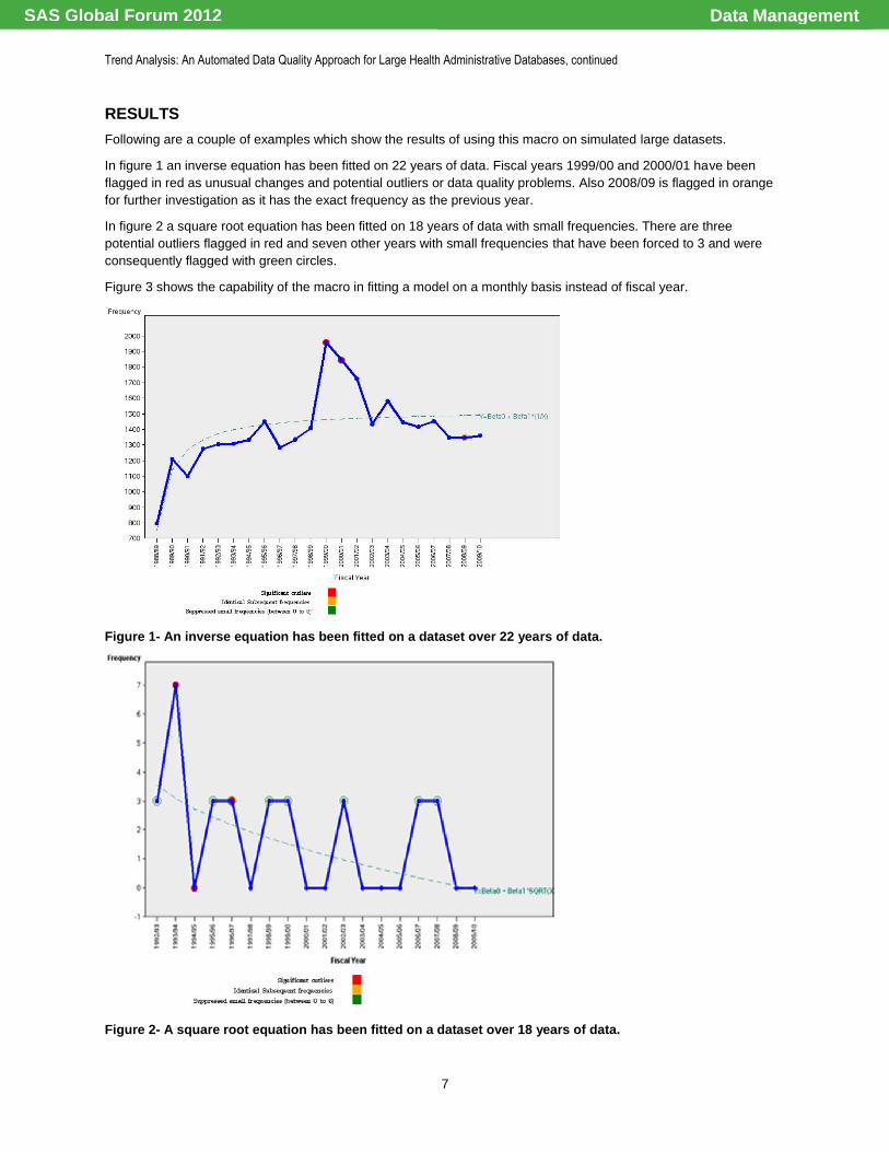
RESULTS

Following are a couple of examples which show the results of using this macro on simulated large datasets.

In figure 1 an inverse equation has been fitted on 22 years of data. Fiscal years 1999/00 and 2000/01 have been

flagged in red as unusual changes and potential outliers or data quality problems. Also 2008/09 is flagged in orange

for further investigation as it has the exact frequency as the previous year.

In figure 2 a square root equation has been fitted on 18 years of data with small frequencies. There are three

potential outliers flagged in red and seven other years with small frequencies that have been forced to 3 and were

consequently flagged with green circles.

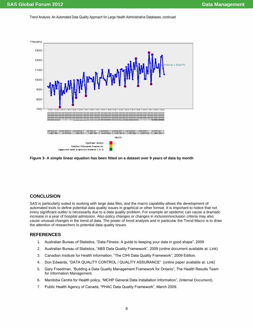
Figure 3 shows the capability of the macro in fitting a model on a monthly basis instead of fiscal year.

Figure 1- An inverse equation has been fitted on a dataset over 22 years of data.

Figure 2- A square root equation has been fitted on a dataset over 18 years of data.

Data ManagementSAS Global Forum 2012

Trend Analysis: An Automated Data Quality Approach for Large Health Administrative Databases, continued

8

Figure 3- A simple linear equation has been fitted on a dataset over 9 years of data by month

CONCLUSION

SAS is particularly suited to working with large data files, and the macro capability allows the development of automated tools to define potential data quality issues in graphical or other format. It is important to notice that not every significant outlier is necessarily due to a data quality problem. For example an epidemic can cause a dramatic increase in a year of hospital admission. Also policy changes or changes in inclusion/exclusion criteria may also cause unusual changes in the trend of data. The power of trend analysis and in particular the Trend Macro is to draw the attention of researchers to potential data quality issues.

REFERENCES

1. Australian Bureau of Statistics, “Data Fitness: A guide to keeping your data in good shape”, 2009

2. Australian Bureau of Statistics, “ABS Data Quality Framework”, 2009 (online document available at: Link)

3. Canadian Institute for Health Information, “The CIHI Data Quality Framework”, 2009 Edition.

4. Don Edwards, “DATA QUALITY CONTROL / QUALITY ASSURANCE” (online paper available at: Link)

5. Gary Freedman, “Building a Data Quality Management Framework for Ontario”, The Health Results Team for Information Management.

6. Manitoba Centre for Health policy, “MCHP General Data Installation Information”, (Internal Document).

7. Public Health Agency of Canada, “PHAC Data Quality Framework”, March 2009.

Data ManagementSAS Global Forum 2012

Trend Analysis: An Automated Data Quality Approach for Large Health Administrative Databases, continued

9

8. UK’s National Health Services, Data Quality Report for Independent Sector NHS funded treatment Q1 – Q2 2007/08 (online document available at: Link)

9. Ron Cody, Cody’s Data Cleaning Techniques Using SAS, SAS Inc., 2008.

ACKNOWLEDGMENTS

Author would like to thank Mr. Mark Smith, Associate Director (Repository) at the Manitoba Centre for Health Policy for his great support and invaluable advice on this project.

CONTACT INFORMATION

Your comments and questions are greatly appreciated and encouraged. The complete macro codes are available through email. Please contact the author at: Mahmoud Azimaee Institute for Clinical Evaluative Sciences (ICES) G1-44, 2075 Bayview Ave, Toronto, ON, M4N 3M5 Work phone: (416) 480 - 4055 (Ex 3618), E-mail: azimaee@gmail.com Web: www.dastneveshteha.com

SAS and all other SAS Institute Inc. product or service names are registered trademarks or trademarks of SAS Institute Inc. in the USA and other countries. ® indicates USA registration.

Other brand and product names are trademarks of their respective companies.

Data ManagementSAS Global Forum 2012