12. Longitudinal - 2016 - Princeton Universitystengel/MAE331Lecture12.pdfyy "!= q Nonlinear Dynamic...

Linearized Longitudinal Equations of Motion!

Robert Stengel, Aircraft Flight Dynamics !MAE 331, 2016

•! 6th-order -> 4th-order -> hybrid equations•! Dynamic stability derivatives •! Long-period (phugoid) mode•! Short-period mode

Copyright 2016 by Robert Stengel. All rights reserved. For educational use only.http://www.princeton.edu/~stengel/MAE331.html

http://www.princeton.edu/~stengel/FlightDynamics.html

Reading:!Flight Dynamics!

452-464, 482-486!

1

Learning Objectives

Review Questions!!! How do numerical integration algorithms work?!!! What’s the difference between a “nominal” and an

“actual” trajectory?!!! What assumptions must be made to derive a set of

linear differential equations from a set of nonlinear equations?!

!! How is a nonlinear spring modeled?!!! What is a “Jacobian matrix”?!!! Does the point of linearization have to be fixed?!!! How are the equations of motion divided into

longitudinal and lateral-directional sets?!!! Why is it useful to do this?!

2

6th-Order Longitudinal Equations of Motion

Symmetric aircraftMotions in the vertical plane

Flat earth

x1x2x3x4x5x6

!

"

########

$

%

&&&&&&&&

= xLon6

!u = X /m ! gsin" ! qw!w = Z /m + gcos" + qu!xI = cos"( )u + sin"( )w!zI = !sin"( )u + cos"( )w

!q = M / Iyy!" = q

State Vector, 6 componentsNonlinear Dynamic Equations

Fairchild-Republic A-10

3

uwxzq!

"

#

$$$$$$$

%

&

'''''''

=

Axial VelocityVertical Velocity

RangeAltitude(–)Pitch RatePitch Angle

"

#

$$$$$$$$

%

&

''''''''

Range has no dynamic effectAltitude effect is minimal (air density variation)

4th-Order Longitudinal Equations of Motion

!u = f1 = X /m ! gsin" ! qw!w = f2 = Z /m + gcos" + qu

!q = f3 = M / Iyy!" = f4 = q

x1x2x3x4

!

"

#####

$

%

&&&&&

= xLon4

State Vector, 4 components

Nonlinear Dynamic Equations, neglecting range and altitude

4

uwq!

"

#

$$$$

%

&

''''

=

Axial Velocity, m/sVertical Velocity, m/sPitch Rate, rad/sPitch Angle, rad

"

#

$$$$$

%

&

'''''

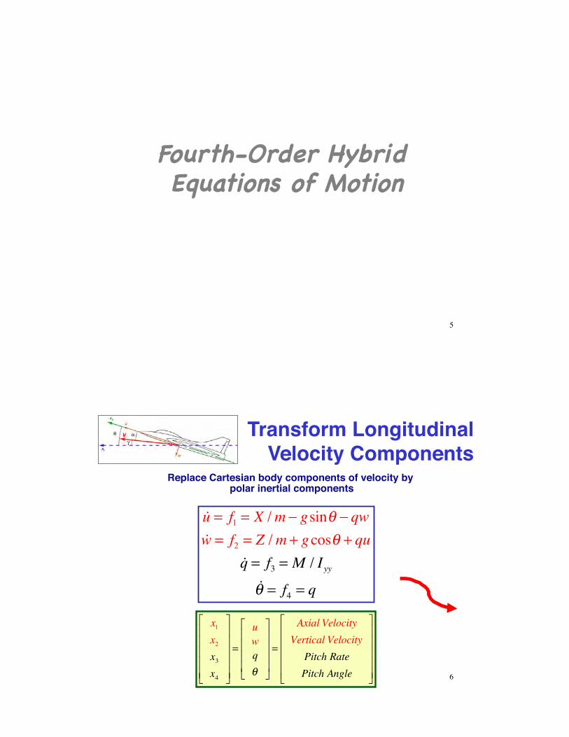
Fourth-Order Hybrid Equations of Motion!

5

Transform Longitudinal Velocity Components

!u = f1 = X /m ! gsin" ! qw!w = f2 = Z /m + gcos" + qu

!q = f3 = M / Iyy!" = f4 = q

x1x2x3x4

!

"

#####

$

%

&&&&&

=

uwq'

!

"

####

$

%

&&&&

=

Axial VelocityVertical Velocity

Pitch RatePitch Angle

!

"

#####

$

%

&&&&& 6

Replace Cartesian body components of velocity by polar inertial components

Transform Longitudinal Velocity Components

!V = f1 = T cos ! + i( )" D "mgsin#$% &' m

!# = f2 = T sin ! + i( ) + L "mgcos#$% &' mV!q = f3 = M / Iyy!( = f4 = q

x1x2x3x4

!

"

#####

$

%

&&&&&

=

V'q(

!

"

####

$

%

&&&&

=

VelocityFlight Path Angle


!

"

#####

$

%

&&&&&

i = Incidence angle of the thrust vectorwith respect to the centerline

7

Hawker P1127 Kestral

Replace Cartesian body components of velocity by polar inertial components

Hybrid Longitudinal Equations of Motion

!V = f1 = T cos ! + i( )" D "mgsin#$% &' m

!# = f2 = T sin ! + i( ) + L "mgcos#$% &' mV!q = f3 = M / Iyy!( = f4 = q

x1x2x3x4

!

"

#####

$

%

&&&&&

=

V'q(

!

"

####

$

%

&&&&

=



!

"

#####

$

%

&&&&& 8

•! Replace pitch angle by angle of attack ! = " # $

Hybrid Longitudinal Equations of Motion

!V = f1 = T cos ! + i( )" D "mgsin#$% &' m

!# = f2 = T sin ! + i( ) + L "mgcos#$% &' mV!q = f3 = M / Iyy

!! = !( " !# = f4 = q " f2 = q "1mV

T sin ! + i( ) + L "mgcos#$% &'

x1x2x3x4

!

"

#####

$

%

&&&&&

=

V'q(

!

"

####

$

%

&&&&

=


Pitch RateAngle of Attack

!

"

#####

$

%

&&&&&

•! Replace pitch angle by angle of attack ! = " # $

! =" +# 9

Why Transform Equations and State Vector?

Velocity and flight path angle typically have slow variations

Pitch rate and angle of attack typically have quicker variations

x1x2x3x4

!

"

#####

$

%

&&&&&

=

V'q(

!

"

####

$

%

&&&&

=


Pitch RateAngle of Attack

!

"

#####

$

%

&&&&&

10

Coupling typically small

Small Perturbations from Steady Path

!x(t) = !xN (t)+ !!x(t)" f[xN (t),uN (t),wN (t),t]+ F t( )!x(t)+G t( )!u(t)+L t( )!w(t)

11

!xN (t) ! 0 " f[xN (t),uN (t),wN (t),t]#!x(t) " F#x(t)+G#u(t)+L#w(t)

Steady, Level Flight

Rates of change are “small”

Nominal Equations of Motion in Equilibrium (Trimmed Condition)

!xN (t) = 0 = f[xN (t),uN (t),wN (t),t]

!VN = 0 = f1 = T cos !N + i( )" D "mgsin# N$% &' m

!# N = 0 = f2 = T sin !N + i( ) + L "mgcos# N$% &' mVN!qN = 0 = f3 = M Iyy

!!N = 0 = f4 = 0( )" 1mVN

T sin !N + i( ) + L "mgcos# N$% &'

T, D, L, and M contain state, control, and disturbance effects

xNT = VN ! N 0 "N

#$

%&

T= constant

12(See Supplemental Material for trimmed solution)

Small Perturbations from Steady Path Approximated by Linear Equations

13

Linearized Equations of Motion

!!xLon =

! !V! !"! !q! !#

$

%

&&&&&

'

(

)))))

= FLon

!V!"!q!#

$

%

&&&&

'

(

))))

+GLon

!*T!*E"

$

%

&&&

'

(

)))+"

Linearized !Equations of Motion!

14

Phugoid (Long-Period) Motion!

Short-Period Motion!

Approximate Decoupling of Fast and Slow Modes of Motion

Hybrid linearized equations allow the two modes to be examined separately

FLon =FPh FSP

Ph

FPhSP FSP

!

"##

$

%&&

Effects of phugoid perturbations on phugoid motion

Effects of phugoid perturbations on

short-period motion

Effects of short-period perturbations on phugoid motion

Effects of short-period perturbations on short-

period motion

=FPh smallsmall FSP

!

"##

$

%&&'

FPh 00 FSP

!

"##

$

%&& 15

Sensitivity Matrices for Longitudinal LTI Model

!!xLon (t) = FLon!xLon (t) +GLon!uLon (t) + LLon!wLon (t)

FLon =

F11 F12 F13 F14F21 F22 F23 F24F31 F32 F33 F34F41 F42 F43 F44

!

"

#####

$

%

&&&&&

GLon =

G11 G12 G13G21 G22 G23

G31 G32 G33

G41 G42 G43

!

"

#####

$

%

&&&&&

LLon =

L11 L12L21 L22L31 L32L41 L42

!

"

#####

$

%

&&&&&

16

Velocity Dynamics

!V = f1 =1mT cos! " D "mgsin#[ ]

= 1m

CT cos!$V 2

2S "CD

$V 2

2S "mgsin#%

&'

(

)*

First row of nonlinear equation

First row of linearized equation

! !V (t) = F11!V (t)+ F12!" (t)+ F13!q(t)+ F14!# (t)[ ]+ G11!$E(t)+G12!$T (t)+G13!$F(t)[ ]

+ L11!Vwind + L12!#wind[ ]

17

F11 =1m

CTVcos!N "CDV( ) #NVN

2

2S + CTN

cos!N "CDN( )#NVNS$

%&

'

()

Coefficients in first row of F

Sensitivity of Velocity Dynamics to State Perturbations

CTV!"CT

"V

CDV!"CD

"V

CDq!"CD

"q

CD#!"CD

"#

!V = CT cos! "CD( ) #V

2

2S "mgsin$

%

&'

(

)* m

18

F12 = !gcos" N

F13 =!1m

CDq

"NVN2

2S#

$%

&

'(

F14 =!1m

CTNsin"N +CD"( ) #NVN

2

2S$

%&

'

()

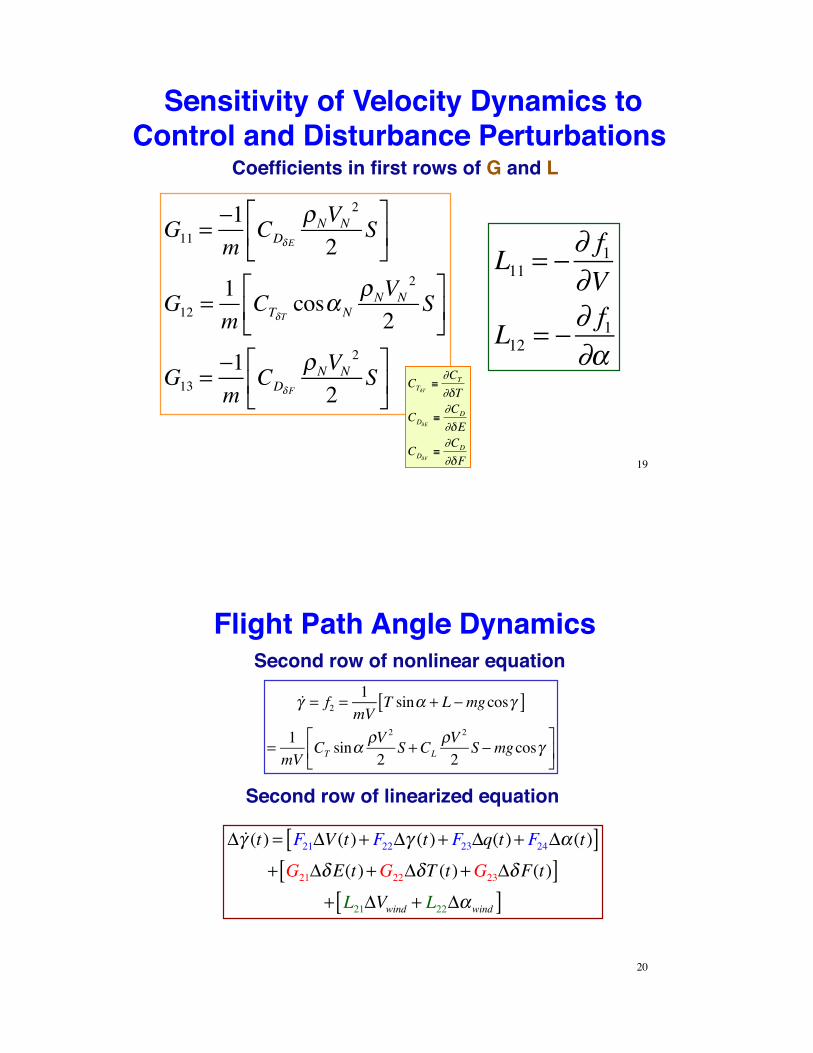
Sensitivity of Velocity Dynamics to Control and Disturbance Perturbations

G11 =!1m

CD"E

#NVN2

2S$

%&

'

()

G12 =1m

CT"Tcos*N

#NVN2

2S$

%&

'

()

G13 =!1m

CD"F

#NVN2

2S$

%&

'

()

Coefficients in first rows of G and L

L11 = ! " f1"V

L12 = ! " f1"#

CT!T"#CT

#!T

CD!E"#CD

#!E

CD!F"#CD

#!F 19

Flight Path Angle Dynamics

Second row of linearized equation

!! = f2 =1mV

T sin" + L #mgcos![ ]

= 1mV

CT sin"$V 2

2S +CL

$V 2

2S #mgcos!%

&'

(

)*

! !" (t) = F21!V (t)+ F22!" (t)+ F23!q(t)+ F24!# (t)[ ]+ G21!$E(t)+G22!$T (t)+G23!$F(t)[ ]


20

Second row of nonlinear equation

F21 =1

mVNCTV

sin!N +CLV( ) "NVN2

2S + CTN

sin!N +CLN( )"NVNS#

$%

&

'(

) 1mVN

2 CTNsin!N +CLN( ) "NVN

2

2S )mgcos* N

#

$%

&

'(

Coefficients in second row of F

Sensitivity of Flight Path Angle Dynamics to State Perturbations

CTV!"CT

"V

CLV!"CL

"V

CLq!"CL

"q

CL#!"CL

"#

!! = CT sin" +CL( ) #V

2

2S $mgcos!

%

&'

(

)* mV

21

F22 = gsin! N VN

F23 =1

mVNCLq

!NVN2

2S"

#$

%

&'

F24 =1

mVNCTN

cos!N +CL!( ) "NVN2

2S#

$%

&

'(

Pitch Rate Dynamics

!q = f3 =

MIyy

=Cm !V 2 2( )Sc

Iyy

Third row of nonlinear equation

Third row of linearized equation

! !q(t) = F31!V (t)+ F32!" (t)+ F33!q(t)+ F34!# (t)[ ]+ G31!$E(t)+G32!$T (t)+G33!$F(t)[ ]


22

F31 =1Iyy

CmV

!NVN2

2Sc +CmN

!NVNSc"

#$

%

&'

Coefficients in third row of F

Sensitivity of Pitch Rate Dynamics to State Perturbations

CmV!"Cm

"V

Cmq!"Cm

"q

Cm#!"Cm

"#

!q =Cm !V 2 2( )Sc Iyy

23

F32 = 0

F33 =1Iyy

Cmq

!NVN2

2Sc"

#$

%

&'

F34 =1Iyy

Cm!

"NVN2

2Sc#

$%

&

'(

Angle of Attack Dynamics

!! = f4 = !" # !$ = q #

1mV

T sin! + L # mgcos$[ ]

Fourth row of nonlinear equation

Fourth row of linearized equation

! !" (t) = F41!V (t)+ F42!# (t)+ F43!q(t)+ F44!" (t)[ ]+ G41!$E(t)+G42!$T (t)+G43!$F(t)[ ]+ L41!Vwind + L42!"wind[ ]

24

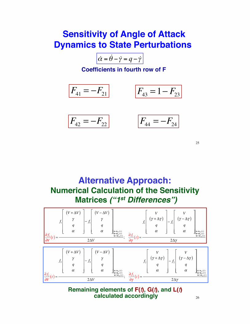
F41 = !F21

Coefficients in fourth row of F

Sensitivity of Angle of Attack Dynamics to State Perturbations

F43 = 1! F23

!! =!" # !$ = q# !$

25

F42 = !F22 F44 = !F24

Alternative Approach: Numerical Calculation of the Sensitivity

Matrices (“1st Differences”)

! f1!V

t( ) "

f1

V + #V( )$q%

&

'

(((((

)

*

+++++

, f1

V , #V( )$q%

&

'

(((((

)

*

+++++ x=xN (t )u=uN (t )w=wN (t )

2#V; ! f1

!$t( ) "

f1

V$ + #$( )q%

&

'

(((((

)

*

+++++

, f1

V$ , #$( )q%

&

'

(((((

)

*

+++++ x=xN (t )u=uN (t )w=wN (t )

2#$

26

Remaining elements of F(t), G(t), and L(t) calculated accordingly

! f2!V

t( ) "

f2

V + #V( )$q%

&

'

(((((

)

*

+++++

, f2

V , #V( )$q%

&

'

(((((

)

*

+++++ x=xN (t )u=uN (t )w=wN (t )

2#V; ! f2

!$t( ) "

f2

V$ + #$( )q%

&

'

(((((

)

*

+++++

, f2

V$ , #$( )q%

&

'

(((((

)

*

+++++ x=xN (t )u=uN (t )w=wN (t )

2#$

Dimensional Stability and Control Derivatives!

27

Dimensional Stability-Derivative Notation

!! Redefine force and moment symbols as acceleration symbols

!! Dimensional stability derivatives portray acceleration sensitivities to state perturbations

Dragmass (m)

! D " !V

Liftmass

! L "V !#

Momentmoment of inertia (Iyy )

! M " !q

28

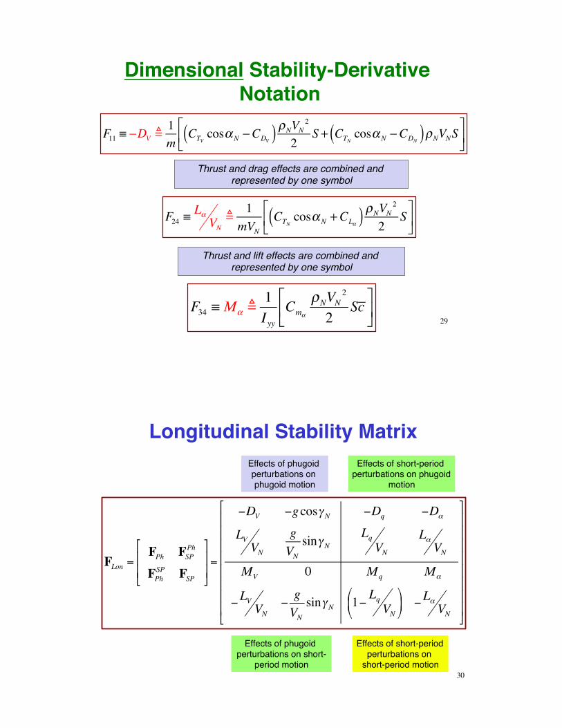
Dimensional Stability-Derivative Notation

F11 ! "DV !

1m

CTVcos#N "CDV( ) $NVN

2

2S + CTN

cos#N "CDN( )$NVNS%

&'

(

)*

F24 !

L"VN!

1mVN

CTNcos"N +CL"( ) #NVN

2

2S$

%&

'

()

F34 ! M" !

1Iyy

Cm"

#NVN2

2Sc$

%&

'

()

Thrust and drag effects are combined and represented by one symbol

Thrust and lift effects are combined and represented by one symbol

29

Longitudinal Stability Matrix

FLon =FPh FSP

Ph

FPhSP FSP

!

"

##

$

%

&&=

'DV 'gcos(N 'Dq 'D)

LVVN

gVNsin(N

LqVN

L)VN

MV 0 Mq M)

'LV VN'gVNsin(N 1' Lq VN

*

+,

-

./ 'L) VN

!

"

########

$

%

&&&&&&&&

Effects of phugoid perturbations on phugoid motion

Effects of phugoid perturbations on short-

period motion

Effects of short-period perturbations on phugoid

motion

Effects of short-period perturbations on

short-period motion30

Curtiss Autocar, 1917 Waterman Arrowbile, 1935

ConsolidatedVultee 111, 1940sStout Skycar, 1931

31

Hallock Road Wing , 1957

ConvAIRCAR 116 (w/Crosley auto), 1940s Taylor AirCar, 1950s

32

Mitzar SkyMaster Pinto, 1970s

Haynes Skyblazer, concept, 2004

Lotus Elise Aerocar, concept, 2002

33

Aeromobil, 2014

Pinto separated from the airframe. Two killed. Proposed, not built.

Proposed, not built.Aircraft entered a spin, ballistic

parachute was deployed. No fatality.

Terrafugia Transition

… or, for the same price

Terrafugia TF-X, concept

PLUS

Jaguar F Type

34

Tecnam Astore

Comparison of 2nd- and 4th-Order Model Response!

35

0 - 100 sec•! Reveals Phugoid Mode

4th-Order Initial-Condition Responses of Business Jet at Two Time Scales

0 - 6 sec•! Reveals Short-Period Mode

Plotted over different periods of time4 initial conditions [V(0), !(0), q(0), "(0)]

36

2nd-Order Models of Longitudinal Motion

Approximate Phugoid Equation

!!xPh =

! !V! !"

#

$%%

&

'(()

*DV *gcos" N

LVVN

gVNsin" N

#

$

%%%

&

'

(((

!V!"

#

$%%

&

'((

+T+TL+T

VN

#

$

%%%

&

'

(((!+T +

*DV

LVVN

#

$

%%%

&

'

(((!Vwind

Assume off-diagonal blocks of (4 x 4) stability matrix are negligible

FLon =FPh ~ 0~ 0 FSP

!

"##

$

%&&

37

2nd-Order Models of Longitudinal Motion

!!xSP =

! !q! !"

#

$%%

&

'(()

Mq M"

1* Lq VN+,-

./0 * L"

VN

#

$

%%%

&

'

(((

!q!"

#

$%%

&

'((

+M1E

*L1EVN

#

$

%%%

&

'

(((!1E +

M"

*L"VN

#

$

%%%

&

'

(((!"wind

Approximate Short-Period Equation

FLon =FPh ~ 0~ 0 FSP

!

"##

$

%&&

38

Comparison of Bizjet 4th- and 2nd-Order Model Responses

39

4th Order,4 initial conditions

[V(0), !(0), q(0), "(0)]

2nd Order,2 initial conditions

[V(0), !(0)]

Phugoid Time Scale, ~100 s

Short-Period Time Scale, ~10 s

Comparison of Bizjet 4th- and 2nd-Order Model Responses

40

4th Order,4 initial conditions

[V(0), !(0), q(0), "(0)]

2nd Order,2 initial conditions

[q(0), "(0)]

Approximate Phugoid Response to a 10% Thrust Increase

What is the steady-state response?41

Approximate Short-Period Response to a 0.1-Rad Pitch Control Step Input

Pitch Rate, rad/s Angle of Attack, rad

42

What is the steady-state response?

Normal Load Factor Response to a 0.1-Rad Pitch Control Step Input

Normal Load Factor, g s at c.m.Aft Pitch Control (Elevator)

Normal Load Factor, g s at c.m.Forward Pitch Control (Canard)

!nz =

VNg

! !" # !q( ) = VNg

L"

VN!" + L$E

VN!$E

%&'

()*

•! Normal load factor at the center of mass

•! Pilot focuses on normal load factor during rapid maneuvering

Grumman X-29

43

Next Time:!Lateral-Directional Dynamics!

Reading:!Flight Dynamics!

574-591!

44

Learning Objectives

•! 6th-order -> 4th-order -> hybrid equations•! Dynamic stability derivatives •! Dutch roll mode•! Roll and spiral modes

SSuupppplleemmeennttaall MMaatteerriiaall

45

Trimmed Solution of the Equations of Motion!

46

Flight Conditions for Steady, Level Flight

!V = f1 =1m

T cos ! + i( ) " D " mgsin#$% &'

!# = f2 =1mV

T sin ! + i( ) + L " mgcos#$% &'

!q = f3 = M / Iyy

!! = f4 = !( " !# = q "1mV

T sin ! + i( ) + L " mgcos#$% &'

Nonlinear longitudinal model

Nonlinear longitudinal model in equilibrium

0 = f1 =1m

T cos ! + i( ) " D " mgsin#$% &'

0 = f2 =1mV

T sin ! + i( ) + L " mgcos#$% &'

0 = f3 = M / Iyy

0 = f4 = !( " !# = q "1mV

T sin ! + i( ) + L " mgcos#$% &' 47

Numerical Solution for Level Flight Trimmed Condition

•!Specify desired altitude and airspeed, hN and VN•!Guess starting values for the trim parameters, !!T0, !!E0, and ""0•!Calculate starting values of f1, f2, and f3

•! f1, f2, and f3 = 0 in equilibrium, but not for arbitrary !!T0, !!E0, and ""0•!Define a scalar, positive-definite trim error cost function, e.g.,

f1 = !V = 1m

T !T ,!E," ,h,V( )cos # + i( )$ D !T ,!E," ,h,V( )%& '(

f2 = !) = 1mVN

T !T ,!E," ,h,V( )sin # + i( ) + L !T ,!E," ,h,V( )$mg%& '(

f3 = !q = M !T ,!E," ,h,V( ) / Iyy

J !T ,!E,"( ) = a f12( )+b f2

2( )+ c f32( )

48

Minimize the Cost Function with Respect to the Trim Parameters

Cost is minimized at bottom of bowl, i.e., when

! J!"T

! J!"E

! J!#

$

%&

'

()= 0

Error cost is bowl-shaped

Search to find the minimum value of J

J !T ,!E,"( ) = a f12( )+b f2

2( )+ c f32( )

49

Example of Search for Trimmed Condition (Fig. 3.6-9, Flight Dynamics)

In MATLAB, use fminsearch to find trim settings

!T*,!E*," *( ) = fminsearch J, !T ,!E,"( )#$ %&50

Elements of the Stability Matrix

! f1!V

" #DV ;! f1!$

= #gcos$ N ;! f1!q

" #Dq;! f1!%

" #D%

! f2!V

" LV VN; ! f2

!#=gVNsin# N ;

! f2!q

"LqVN; ! f2

!$" L$ VN

! f3!V

" MV ;! f3!#

= 0; ! f3!q

" Mq;! f3!$

" M$

! f4!V

" # LV VN; ! f4

!$= #

gVNsin$ N ;

! f4!q

" 1# Lq VN; ! f4

!%" # L% VN

Stability derivatives portray acceleration sensitivities to state perturbations

51

! f2!"E

=1

mVNCL"E

#VN2

2S

$

%&

'

()

! f2!"T

=1

mVNCT"T

sin*N#VN

2

2S

$

%&

'

()

! f2!"F

=1

mVNCL"F

#VN2

2S

$

%&

'

()

! f2!Vwind

= "! f2!V

! f2!#wind

= "! f2!#

Control and Disturbance Sensitivities in Flight Path Angle, Pitch Rate, and

Angle-of-Attack Dynamics! f3!"E

=1Iyy

Cm"E

#VN2

2Sc

$

%&

'

()

! f3!"T

=1Iyy

Cm"T

#VN2

2Sc

$

%&

'

()

! f3!"F

=1Iyy

Cm"F

#VN2

2Sc

$

%&

'

()

! f3!Vwind

= "! f3!V

! f3!#wind

= "! f3!#

! f4!"E

= #! f2!"E

! f4!"T

= #! f2!"T

! f4!"F

= #! f2!"F

! f4!Vwind

=! f2!V

! f3!"wind

=! f2!" 52

Velocity-Dependent Derivative Definitions

Air compressibility effects are a principal source of velocity dependence

CDM!"CD

"M=

"CD

" V / a( )= a "CD

"V

CDV!"CD

"V=1a#

$%&

'(CDM

CLV!"CL

"V=1a#

$%&

'(CLM

CmV!"Cm

"V=1a#

$%&

'(CmM

CDM! 0

CDM> 0 CDM

< 0

a = Speed of Sound

M = Mach number = V a

53

Wing Lift and Moment Coefficient Sensitivity to Pitch Rate

Straight-wing incompressible flow estimate (Etkin)CLq̂wing

= !2CL"winghcm ! 0.75( )

Cmq̂wing= !2CL"wing

hcm ! 0.5( )2

Straight-wing supersonic flow estimate (Etkin)CLq̂wing

= !2CL"winghcm ! 0.5( )

Cmq̂wing= ! 2

3 M 2 !1! 2CL"wing

hcm ! 0.5( )2

Triangular-wing estimate (Bryson, Nielsen)

CLq̂wing= ! 2"

3CL#wing

Cmq̂wing= ! "

3AR54

Control- and Disturbance-Effect Matrices

•! Control-effect derivatives portray acceleration sensitivities to control input perturbations

•! Disturbance-effect derivatives portray acceleration sensitivities to disturbance input perturbations

GLon =

!D"E T"T !D"F

L"E /VN L"T /VN L"F /VNM"E M"T M"F

!L"E /VN !L"T /VN !L"F /VN

#

$

%%%%%

&

'

(((((

LLon =

!DVwind!D"wind

LVwind /VN L"wind /VNMVwind

M"wind

!LVwind /VN !L"wind /VN

#

$

%%%%%%

&

'

(((((( 55

Primary Longitudinal Stability Derivatives

DV !

!1m

CTV!CDV( ) "VN

2

2S+ CTN

!CDN( )"VNS#

$%

&

'(

Small angle assumptions

LVVN!

1mVN

CLV

!VN2

2S + CLN

!VNS"

#$

%

&' (

1mVN

2 CLN

!VN2

2S ( mg

"

#$

%

&'

Mq =1Iyy

Cmq

!VN2

2Sc

"

#$

%

&' M! =

1Iyy

Cm!

"VN2

2Sc

#

$%

&

'(

L!VN!

1mVN

CTN+ CL!( ) "VN

2

2S

#

$%

&

'(

56

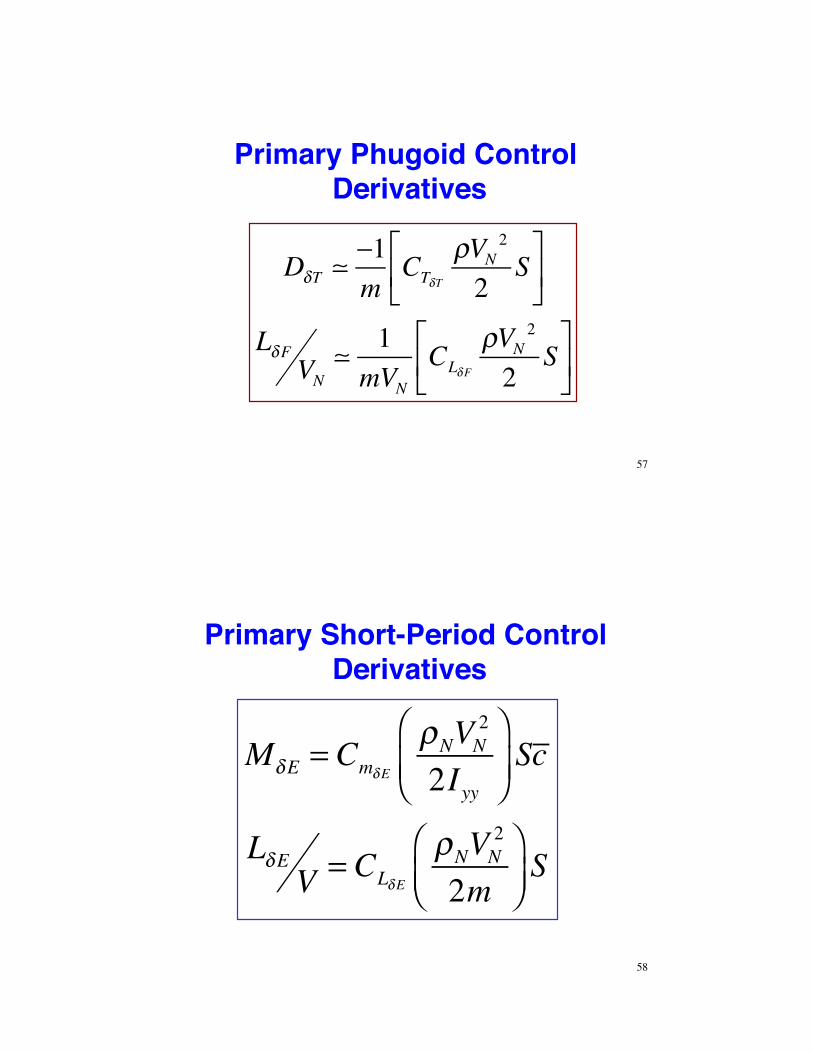
Primary Phugoid Control Derivatives

D!T !"1m

CT!T

#VN2

2S$

%&

'

()

L!FVN!

1mVN

CL!F

#VN2

2S$

%&

'

()

57

Primary Short-Period Control Derivatives

M!E = Cm!E

"NVN2

2Iyy

#

$%&

'(Sc

L!EV = CL!E

"NVN2

2m#$%

&'(S

58

Flight Motions

Dornier Do-128 Short-Period Demonstrationhttp://www.youtube.com/watch?v=3hdLXE0rc9Q

Dornier Do-128D

Dornier Do-128 Phugoid Demonstrationhttp://www.youtube.com/watch?v=jzxtpQ30nLg&feature=related

59

12. Longitudinal - 2016 - Princeton Universitystengel/MAE331Lecture12.pdfyy "!= q Nonlinear Dynamic...

Documents

Transcript of 12. Longitudinal - 2016 - Princeton Universitystengel/MAE331Lecture12.pdfyy "!= q Nonlinear Dynamic...