12. Interaction of Radiation with Matter - MIT OpenCourseWare · 12. Interaction of Radiation with...

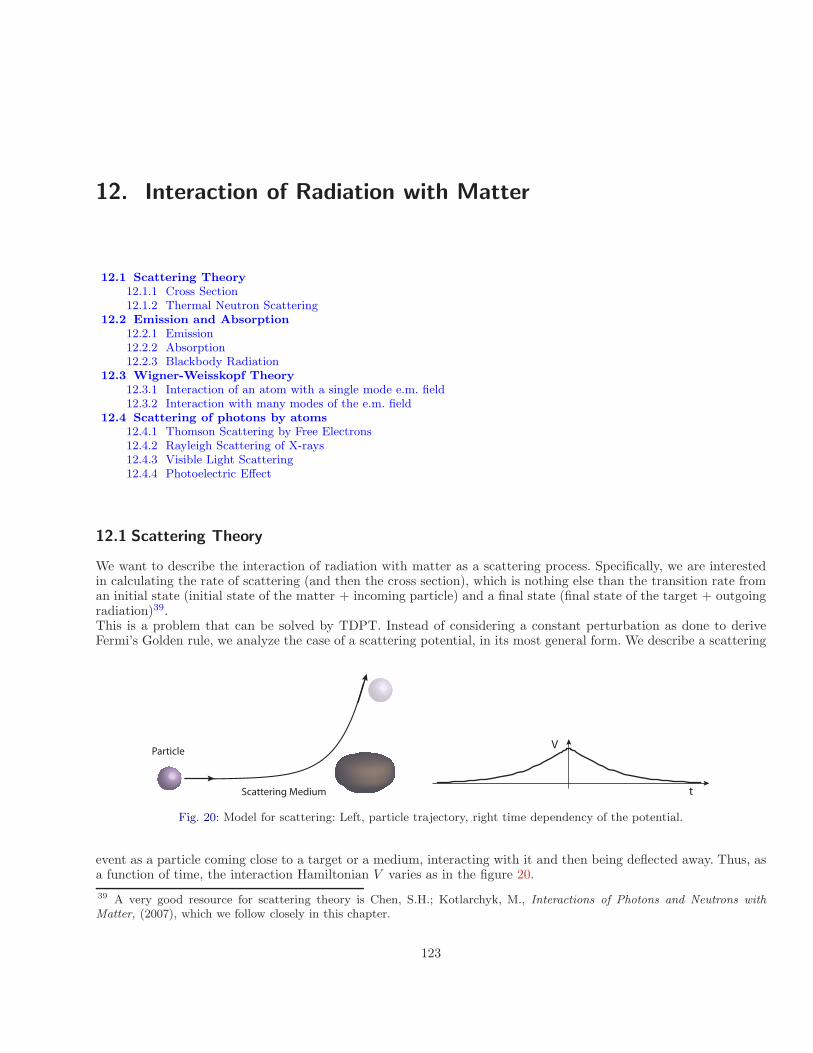
12 Interaction of Radiation with Matter

121 Scattering Theory 1211 Cross Section 1212 Thermal Neutron Scattering

122 Emission and Absorption 1221 Emission 1222 Absorption 1223 Blackbody Radiation

123 Wigner-Weisskopf Theory 1231 Interaction of an atom with a single mode em field 1232 Interaction with many modes of the em field

124 Scattering of photons by atoms 1241 Thomson Scattering by Free Electrons 1242 Rayleigh Scattering of X-rays 1243 Visible Light Scattering 1244 Photoelectric Effect

121 Scattering Theory

We want to describe the interaction of radiation with matter as a scattering process Specifically we are interested in calculating the rate of scattering (and then the cross section) which is nothing else than the transition rate from an initial state (initial state of the matter + incoming particle) and a final state (final state of the target + outgoing radiation)39 This is a problem that can be solved by TDPT Instead of considering a constant perturbation as done to derive Fermirsquos Golden rule we analyze the case of a scattering potential in its most general form We describe a scattering

Particle

Scattering Medium

V

t

Fig 20 Model for scattering Left particle trajectory right time dependency of the potential

event as a particle coming close to a target or a medium interacting with it and then being deflected away Thus as a function of time the interaction Hamiltonian V varies as in the figure 20

39 A very good resource for scattering theory is Chen SH Kotlarchyk M Interactions of Photons and Neutrons with

Matter (2007) which we follow closely in this chapter

123

We want to calculate the probability of scattering from an initial state to a final state

I infin Pscatt = | (f |UI (t) |i) |2 = | (f | (11minus i VI (t prime )dt prime + ) |i) |2

minusinfin

Notice that we consider negative times as well This corresponds to the so-called adiabatic switching since the interaction is assumed to be turned on slowly from the beginning of time and to go down to zero again for long times

A Scattering and Transition matrices

In scattering problems the propagator UI is usually called the scattering matrix S To simplify the calculation we can assume again that V is actually time-independent Then from the first order TDPT we obtain

(f |S(1) |i) I infin

iωfitdt == minusiVfi e minus2πiδ(ωf minus ωi)Vfi minusinfin

Now consider the second order contribution

t1


iωfmt1

I iωmit2= minus (f | V |m) (m|V |i) dt1e dt2e

minusinfin minusinfinm

Notice that the last integral is not well defined for t rarr minusinfin To solve it we rewrite it as

t1 iωmit+ǫtI

i(ωmiminusiǫ)t2 e t1

ǫrarr0+ minusinfin ǫrarr0+ ωmi minus iǫ lim dt2e = lim minusi minusinfin

Now when taking the limit t rarr minusinfin the exponential term eǫt rarr 0 (thus getting rid of the oscillations) Then we are left with only

t1 i(ωmiminusiǫ)t1I eiωmit2dt2e = lim minusi

minusinfin ǫrarr0+ ωmi minus iǫ

and we obtain (setting now ǫ = 0)

(f |S(2) |i) I infin ei(ωfiminusiǫ)t1 (f |V |m) (m|V |i)

= i

VfmVmi dt1 = minus2πiδ(ωf minus ωi)

minusinfin ωmi minus iǫ ωi minus ωm m m

Looking at the first and second order of the scattering matrix we start seeing a pattern emerge We can thus rewrite

(f |S |i) = minus2πiδ(ωf minus ωi) (f |T |i)

where T is called the transition matrix Its expansion is given by

(f |V |m) (m|V |i) VfmVmnVni(f |T |i) = (f |V |i)+

+

+ ωi minus ωm (ωi minus ωm)(ωi minus ωn)m mn

B Scattering Probability

We can now turn to calculate the scattering probability PS = | (f |S |i) |2 In order to obtain the total scattering probability we will need to consider all possible final states We found

Ps = 4π2| (f |T |i) |2δ2(ωf minus ωi)

124

We calculate the square of the Dirac function from its definition based on the limit of the integral

1 I infin 1

I infin t δ2(ω) = dteiωtδ(ω) = dtδ(ω) = lim δ(ω)

2π 2π trarrinfin πminusinfin minusinfin

Then although the probability is not so well defined since it contains a limit

Ps = lim 4πt| (f |T |i) |2δ(ωf minus ωi) trarrinfin

the rate of scattering is well defined since it is WS = PS (2t)

WS = 2π| (f |T |i) |2δ(ωf minus ωi)

This is the rate for one isolated final state If instead we have a continuum of final states with density of states ρ(ωf ) we need to sum over all possible final states

WS = 2π I

2π| (f |T |i) |2δ(ωf minus ωi)ρ(ωf )dωf = 2π| (f |T |i) |2ρ(ωi)

Notice that to first order this is equivalent to the Fermi Golden rule

1211 Cross Section

We now use the tools developed in TDPT to calculate the scattering cross section This is defined as the rate of scattering divided by the incoming flux of ldquoparticlesrdquo

d 2σ WS (Ω E)prop d ΩdE Φinc

We consider a particle + medium system where the particle is some radiation represented by a plane wave of

momentum kk In general we will have to define also other degrees of freedom denoted by the index λ eg for photons we will have to define the polarization while for particles (ege neutrons) the spin The unperturbed Hamiltonian is H0 = HR +HM (radiation and medium) We assume that for t rarr plusmninfin the radiation and matter systems are independent with (eigen)states

|i) = |kimi) |f) = |kf mf )

with energies

HR |ki) = hωi |ki) HR |kf ) = hωf |kf ) HM |mi) = ǫi |ki) HM |mf ) = ǫf |mf )

and total energies Ei = hωi + ǫi and Ef = hωf + ǫf

Particle

θ

dΩ

Scattering Medium

125

Scattering Rate

The rate of scattering is given by the expression found earlier

2π Wfi = | (f |T |i) |2δ(Ef minus Ei)

h

As usual we want to replace if possible the delta-function with the final density of states However only the radiation will be left in a continuum of states while the target will be left in one (of possibly many) definite state To describe this distinction we separate the final state into the two subsystems We first define the partial projection on radiation states only Tkf ki = (kf |T |ki) By writing the delta function as an integral we have

2π dagger 1 I infin

i(ωfminusωi)t i(ǫfminusǫi)tWfi = (mf |Tkf ki |mi) (mi|T |mf ) e ekf kih 2πh minusinfin

Now since eminusiHRt |mi) = eminusiǫit |mi) (and similarly for |mf ) we can rewrite

(mf |Tkf ki |mi) e i(ǫfminusǫi)t = (mf | e iHRtTkf kie minusiHRt |mi) = (mf |Tkf ki(t) |mi)

and obtain a new expression for the rate as a correlation of ldquotransitionrdquo events

1 I infin

Wfi = e i(ωfminusωi)t (mi|Tkdagger f ki

(0) |mf ) (mf |Tkf ki(t) |mi)h2 minusinfin

Final density of states

The final density of states describe the available states for the radiation As we assumed that the radiation is represented by plane waves (and assuming for convenience they are contained in a cavity of edge L) the final density of states is (

L )3

ρ(kf )d3kf = kf

2dkf dΩ 2π

We can express this in terms of the energy ρ(k)d3k = ρ(E)dEdΩ For example for photons which have k = Ehc we have (

L )3

E2 ( L )3

ω2 kρ(E) = 2 = 2

2π h3c3 2π hc3

2 k2

where the factor 2 takes into account the possible polarizations For neutrons (or other particles such that E = ) 2m

radic( L )3

k ( L )3

2mE ρ(E) = =

2π h2 2π h3

If the material target can be left in more than one final state we sum over these final states f Then the average rate is given by W S =

LWfiρ(E)dEdΩ (assuming that Wfi does not change very much in dΩ and dE) f

Incoming Flux

The incoming flux is given by the number of scatterer per unit area and unit time Φ = In the cavity considered A t vwe can express the time as t = Lv thus the flux is Φ = For photons this is simply Φ = cL3 while for massive L3

kparticles (neutrons) v = hkm yielding Φ = mL3

126

Average over initial states

If the scatterer is at a finite temperature T it will be in a mixed state thus we need to sum over all possible initial states

minusβHM minusǫikbTe eρi = rarr Pi =

Z L

i eminusǫikbT

We can finally write the total scattering rate as

WS (i rarr Ω + dΩ E + dE) = ρ(E) Pi Wfi

i f

Pi I infin

dagger ρ(E)I infin

dagger

= ρ(E) e iωfit (mi|T (0) |mf ) (mf |Tkf ki(t) |mi) dEdΩ = e iωfit T (0)Tfi(t)kf ki if

h2 h2 minusinfin minusinfin fi

where (middot) indicates an ensemble average at the given temperature

1212 Thermal Neutron Scattering

Using the scattering rate above and the incoming flux and density of state expression we can find the cross section for thermal neutrons From (

L )3

mkf

hki

(mL3)2 kf

ρ(E)Φ = = 2π h2 mL3 (2πh)3 ki

we obtain

I infind 2σ W ρ(E) 1 1 ( mL3

)2 I infin iωfit

T dagger

kf iωfit T dagger

= h = h e (0)Tfi(t) = e (0)Tfi(t)if if dΩdω Φ Φ h2 2π 2πh2 kiminusinfin minusinfin

Now the eigenstates |kif ) are plane waves (r|k) = ψk(r) = eikmiddotr L32 Then defining Q = ki minus kf the transition matrix element is

I 1 I

d3Tfi(t) = (kf |T (t) |ki) = d3rψkf (r) lowast T (r t)ψki(r) = reiQmiddotrT (r t)

L3 L3 L3

and 1 I

Tfi(0)dagger =

L3 d3 re minusiQmiddotrT (r 0)dagger

L3

Fermi Potential

To first order we can approximate T by V the nuclear potential in the center of mass frame (of the neutron+nucleus) You might recall that the nuclear potential is a very strong (V0 sim 30MeV) and narrow (r0 sim 2fm) potential These characteristics seem to preclude a perturbative approach since the assumption of a weak interaction (compared to the unperturbed system energy) is not satisfied Still the fact that the potential is narrow means that the interaction only happens for a very short time Thus if we average over time we expect a weak interaction More precisely the scattering interaction only depends on the so-called scattering length a which is on the order a sim V0r0 If we keep a constant different combinations of V r will give the same scattering behavior We can thus replace the strong nuclear potential with a weaker pseudo-potential V0 provided this has a much longer range r0 such that a sim V0r0 = V0r0 We can choose V0 r0 so that the potential is weak (eV) but the range is still short compared to the wavelength of the incoming neutron kr0 ≪ 1 Then it is possible to replace the potential with a simple delta-function at the origin

2πh2 V (r) = aδ(r)

micro

127

sum sum

sum

micro a asymp A+1 We can also define the bound scattering length b = mn A were mn is the neutronrsquos mass and A the nucleus mass number Then the potential is

2πh2 V (r) = aδ(r)

mn

Note that b (interaction length or bound scattering length) is a function of the potential strength and range which depend on the isotope from which the neutron is scattered off

22πThen to first order the transition matrix is Tfi = b or more generally if there are many scatterers each at a mn

position rx(t) we have 2πh2 iQmiddotrx(t)Tfi(t) = bxemn x

The scattering cross section becomes

d 2σ I infin

1 kf iωfit minusiQmiddotrx(0) iQmiddotry(t)= e bxbye e

d Ωdω 2π ki minusinfin xy

Notice that since the collisions are spin-dependent we should average over isotopes and spin states and replace bxby

with bxby

Scattering Lengths

Notice that b does not depend explicitly on position although the position determines which isotopespin we should 2

consider What is bxby We have two contributions For x = y this is b2δxy while for x y it is b (1 minus δxy= ) We 2 2

then write bxby = (b2 minus b )δxy + b = b2 i + b2 which defines the coherent scattering length bc = b and the incoherent c 2

scattering length b2 = b2 minus b If there are N scatterers we have L bxby = N(bi

2 + b2) i c

Structure Factors

Using these definition we arrive at a simplified expression

kfd 2σ = N

bi 2SS (Q ω) + b2S(Q ω)

cd Ωdω ki

where we used the self-dynamic structure factor

I infin

1

1 iωfit minusiQmiddotrx(0) iQmiddotrx(t)SS (Q ω) = e e e2π Nminusinfin x

which simplifies to 1 I infin

iωfit minusiQmiddotr(0) iQmiddotr(t)SS (Q ω) = e e e2π minusinfin

if all nuclei are equivalent (same isotope) and the full dynamic structure factor

1 I infin

1

iωfit minusiQmiddotrx(0) iQmiddotry(t)S(Q ω) = e e e

2π Nminusinfin xy

The structure factors depend only on the material properties Thus they give information about the material when obtained from experiments

128

sum

sum

6

sum

sum

6

lang rang

Intermediate Scattering Function

From the expressions above for the structure factors it is clear that they can be obtained as the Fourier Transform (with respect to time) of the quantities

1 minusiQmiddotr(0) iQmiddotrx(t)FS (Q t) = e eN

x

and 1 minusiQmiddotrx(0) iQmiddotry(t)F (Q t) = e eN

xy

These are called the intermediate scattering functions Going even further we can write even these function as a Fourier Transform (with respect to position) For example for equivalent targets (no distribution in isotope nor spin) we have

minusiQmiddotr(0) iQmiddotr(t)FS (Q t) = e e

By defining a the position of a test particle n(R t) = δ(R minus r(t)) we can calculate the fourier transform n(Q t) I d3 iQmiddotR iQmiddotr(t)n(Q t) = re n(R t) = e

Then we have FS (Q t) = (n(Q t)n(minusQ 0)) We can as well define the van-Hove space-time self correlation function

I prime prime prime Gs(r t) = d3 r (n(r 0)n(r + r t))

which represents a correlation of the test particle in space-time The intermediate scattering function is obtained from Gs as

FS (Q t) =

I d3 reiQmiddotr Gs(r t)

These final relationship makes it clear that FS is the Fourier transform (with respect to space) of the time-dependent correlation of the test particle density n(R t) which only depends on the target characteristics

Example I Resting free nucleus

We consider the scattering from one resting free nucleus We need only consider the self dynamics factor and we have bc = b = b

d 2σ kf σb kf = b2S(Q ω) = S(Q ω)

d Ωdω ki 2πh ki

where we introduced the bound cross section σb = 4πb2 (with units of an area) Since the nucleus is free the intermediate function is very simple From


we can use the BCH formula to write

minusiQmiddot[r(0)minusr(t)]+ 1 [Qmiddotr(0)Qmiddotr(t)] 2FS (Q t) = e

Then we want to calculate [r(0) r(t)] in order to simplify the product of the two exponential For a free particle r(t) = r(0) + p t and [r(0) p] = ih Then we have m

minusiQmiddot[r(0)minusr(t)]+i Q2 t minusiQmiddotpm +i Q2 t2m 2mFS (Q t) = e = e e

129

langsum

rang

langsum

rang

lang rang

lang rang

lang rang

lang rang lang rang

and for a nucleus at rest (p = 0) we have itQ2 (2m)FS (Q t) = e

This gives the structure factor (hQ2

)Ss(Q ω) = δ ω minus

2m

and the cross-section d 2σ σb kf

(hQ2

)= δ ω minus

d ΩdE 2πh ki 2m

Since Q = minus ki we have Q2 = k2 + k2 minus 2kikf cosϑ Also ω = minus Ei and k2 = 2mEa asymp 2AEa where we kf i f Ef a substituted A for the mass of the nucleus We can then integrate the cross-section over the solid angle to find d σ dE

I Eid σ I π σb kf

(hQ2

) Aσb

= δ ω minus 2π sinϑdϑ = δ(x)dx dE 2πh ki 2m 4Ei0 (Aminus1)2(A+1)2Ei

Defining the free-atom cross section σf (1)minus2

σf = 1 + σbA

we have 2

d σ

(A+1)2 (Aminus1

fσf for E lt Ef lt E = 4AE A+1

dE 0 otherwise

This expression for the cross section can also be obtained more simply from an energy conservation argument

Example II Scattering from a crystal lattice

We consider now the scattering of neutrons from a crystal For simplicity we will consider a one-dimensional crystal lattice modeled as a 1D quantum harmonic oscillator The position r rarr x (in 1D) of a nucleus in the lattice is then the position of an harmonic oscillator of mass M and frequency ω0

J h dagger)x = (a + a

2Mω0

with evolution given by the Hamiltonian

2p Mω2 10 2 daggerH = + x = hω0(a a + )2M 2 2

If we consider no variation of isotope and spin for simplicity we only need the self-intermediate structure function is

1minusiQmiddotx(0) iQmiddotx(t) minusiQmiddot[x(0)minusx(t)] + [Qmiddotx(0)Qmiddotx(t)] 2FS (Q t) = e e = e e

First remember that p(0)

x(t) = x(0) cos(ω0t) + sin(ω0t)Mω0

ifor an harmonic oscillator Then [x(0) x(t)] = [x(0) p(0)] 1 sin(ω0t) = sin(ω0t) Also we have Mω0 Mω0

p(0) J

h minusiω0 t dagger iω0t)∆x(t) = x(t) minus x(0) = x(0)[1 minus cos(ω0t)] + sin(ω0t) = (ae + a e Mω0 2Mω0

130

We want to evaluate (eiQ∆x(t)

) Using again the BCH formula we have

minusiω0 t dagger iω0tiQ (ae +a e ) dagger minusα lowast dagger dagger2Mω0 αaminusα lowast a a αa minus|α|2[aa ]2 e = e = e e e

V minusiω0t minusα lowast a αa with α = iQ e Since [a adagger] = 1 we only need to evaluate the expectation value e

dagger

e by 2Mω0

expanding in series the exponentials

dagger n) αn(minusαlowast)m

minusα lowast a αa daggerm e e = (a a

nm nm

Only the terms with m = n survive (the other terms are not diagonal in the number basis)

dagger n)) (minus|α|2)n

minusα lowast a αa daggern e e = ((a a

(n)2 n

daggern daggerNow (a an

) = n

((a a)n

) thus we finally have

dagger dagger

e minusα lowast a e αa = ((a dagger a)n

) (minus|α|2)n

= eminus|α|2(a a)n

n

(A2)2This result is a particular case of the Bloch identity (eA) = e where A = αa + βadagger is any combination of the

creation and annihilation operators Finally we obtained for the intermediate function

minus Q2 1 1 iQ2

minusiQmiddotx(0) iQmiddotx(t) ((n)+ ) + sin(ω0 t)2Mω0 2 2 Mω0FS (Q t) = e e = e e

(A2 )2We can also rewrite this using the Bloch identity Using the Bloch identity (eA) = e where A = αa + βadagger is

any combination of the creation and annihilation operators we can rewrite this as

1 1minusiQmiddotx(0) iQmiddotx(t) (eiQ∆x

) e + [Qmiddotx(0)Qmiddotx(t)] minusQ2(∆x2 )2 + [Qmiddotx(0)Qmiddotx(t)] 2 2FS (Q t) = e e = = e e

Now (∆x2

) = (x(0)2

) + (x(t)2

) + 2 (x(0)x(t)) minus ([x(0) x(t)]) = 2

(x 2) + 2 (x(0)x(t)) minus ([x(0) x(t)])

from which we obtain minusQ2 (x 2) Q2 (x(0)x(t))FS (Q t) = e e

If the oscillator is in a number state |n) we have

h h iω0t](x 2) = (2n + 1) (x(0)x(t)) = [2n cos(ω0t) + e

2Mω0 2Mω0

If we consider an oscillator at thermal equilibrium we need to replace n with (n) In the high temperature limit th(n) ≫ 1 and we can simplify

Q2 minus (n)[1minuscos(ω0t)] minusQ2 W02 Q2W (t)2FS (Q t) = e Mω0 = e e

2(n)with W0 = Mω0 and W (t) = W0 cos(ω0t) This form of the intermediate function is the same expression one would

minusQ2

obtain from a classical treatment and the term e W0 2 is called the Debye-Waller factor The intermediate structure function is thus a Gaussian function with a time-dependent width W0minusW (t) IfW0 lt 1 we can make an expansion of the time-dependent term

minusQ2 Q2 minusQ2 1W0 2 W0 cos(ω0t)2 asymp W0 2FS (Q t) = e e e 1 +W0 cos(ω0t) + W02 cos 2(ω0t) +

2

131

lang rang

lang rang sum

lang rang sum

lang rang sum

lang rang

[ ]

Then the structure factor which is the Fourier transform of FS will be a sum of Dirac functions at frequencies ω = plusmnnω0 corresponding to the n-phonon contribution to the scattering Here the terms δ(ω minus nω0) correspond to scattering events where the energy has been transfered from the neutron to the oscillator while terms δ(ω + nω0) describe a transfer of energy from the lattice to the neutron The constant term yields δ(ω) which describes no energy exchange or elastic scattering (zero-phonon term) Note that the expansion coefficient W0 can be expressed in terms

kbT 2kbTof the temperature since in the high temperature limit (n) asymp from which W0 = ω0 Mω2

0

In the low temperature limit (n) rarr 0 Thus we have

minus Q2 iω0t Q2 Q2 iω0 t

2Mω0 2(n)[1minuscos(ω0t)]+1minuse minusQ2

2Mω0 e 2Mω0 eFS (Q t) = e asymp e

Expanding in series the second term we have

minusQ2 Q2 hQ2 1 (

hQ2 )2

iω0t 2iω0tFS (Q t) asymp e 2Mω0 1 + e + e + 2Mω0 2 2Mω0

Even at low temperature the structure factor (the Fourier transform of the expression above) is a sum of Dirac function also called a phonon expansion However in this case only terms δ(ω minus nω0) appear since energy can only be given from the neutron to the lattice (which is initially in its ground state)

132

[ ]

122 Emission and Absorption

Atoms and molecules can absorb photons and make a transition from their ground state to an excited level From the excited state they can emit photons (either in the presence or absence of a preexisting em filed) and transition to a lower level Using TDPT and the quantization of the field we can calculate the transition rates

1221 Emission

|engt

|gn+1gt Fig 21 Model for emission the atom (molecule) makes a transition from the excited level (|e) to the ground state )|g) while the number of photons in the mode k λ goes from n to n + 1

The rate of emission is given simply by 2π

W = | (f |V |i) |2ρ(Ef ) h

We separate the field and the atom (or molecule) levels

|i) = |nkλ) |e) |f) = |nkλ + 1) |g)

As we are looking at atomicoptical processes the dipolar approximation is adequate and the interaction is given by

minusk k kV = d middot E = minusekr middot E Remember the expression for the electric field J

2πhωkk(

ikr dagger minusikr fkE = akλe + akλe ǫkλ

L3 kλ

The position of the electron which makes the transition can be written as kr = Rk +ρk where Rk is the nucleus position Since the relative position of the electron with respect to the nucleus is ρ ≪ λ we can neglect it and substitute r with R in the exponential (ρk middot kk ≪ 1) This simplifies the calculation since R is not an operator acting on the electron state Then from the rate

2π kW = | (g| dk|e) middot (nkλ + 1|E |nkλ) |2ρ(Ef )h

we obtain 2(2πe)2 (

ikR dagger minusikRf |nkλ) (g|kW = ωkprime λprime (nkλ + 1| akprime λprime e + akprime λprime e r middot ǫkprime λprime |e) ρ(Ef )

L3 kprime λprime

Since we are creating a photon only terms prop adagger survive and specifically the term with the correct wavevector and radicdaggerpolarization (nkλ + 1|a |nkλ) = nkλ + 1 (all other terms are zero) Then we have kλ

(2πe)2 2W = ωkλ(nkλ + 1) |(g|kr middot ǫkλ |e)| ρ(Ef )

L3

Since the atom is left in a specific final state the density of states is defined by the em field

ρ(Ef )dEf = ρ(hωk)hdωk

133

sum

sum ∣∣∣∣∣∣

3 3 ω2L LAs ωk = ck and ρ(k)d3k = k2dkdΩ = dωdΩ we have 32π 2π c

( L )3

ω2

ρ(E) = dΩ 2π hc3

We define the dipole transition matrix element from the dipole operator dk= ekr dge = (g| d |e) The rate of emission is then

ω3 k kW = (nkλ + 1)|kǫkλ middot dge|2dΩ

2πhc3

From this expression it easy to see that there are two contributions to emission Spontaneous emission

ω3 k kW = |kǫkλ middot dge|2dΩ

2πhc3

which happens even in the vacuum em and stimulated emission

ω3 k kW = nkλ|kǫkλ middot dge|2dΩ

2πhc3

which happens only when there are already n photons of the correct mode

Spontaneous Emission

|e0〉 k

θ

φ

d

ε2

|g1〉 ε1

Fig 22 Geometry of spontaneous emission

Since the photons emitted can have any polarization ǫ and any wavevector kk direction we have to sum over all possibilities We assume that the dipole vector forms an angle ϑ with respect to the wavevector k Then the two possible polarization vectors are perpendicular to k as in Fig 22 The rate is the sum of the rates for each polarization Wsp = W1 + W2 each proportional to |d middot ǫk12|2

d middot ǫk1 = d sinϑ cosϕ d middot ǫk2 = d sinϑ sinϕ

We thus obtain the typical sin2 ϑ angular dependence of dipolar radiation (also seen for classical dipoles)

ω3 kWsp = |dge|2 sin2 ϑdΩ

2πhc3

The total emission coefficient or Einsteinrsquos emission coefficient is obtained by integrating over the solid angle

I ω3 I 1 4 ω3 k k d2Ae = W dΩ = |dge|22π (1 minus micro 2)dmicro = ge

Ω 2πhc3 minus1 3 hc3

134

( ) ( )

Given the rate we can also calculate the power emitted as rate times energy

4 ωk 4

d2 3 c3 ge P = hωkAe =

Notice that this is very similar to the power emitted by a classical oscillating dipole (as if the em field was emitted by orbiting electrons)

Stimulated Emission

In the stimulated emission W kλ = nkλW kλ Only photons with the same frequency (kk) and polarization of the st sp ones already in the field can be emitted Then as more photons in a particular mode are emitted it becomes even more probable to produce photons in the same mode we produce a beam of coherent photons (ie all with the same characteristics and phase coherent with each other) If the atoms can be kept in the excited (emitting) levels we obtain a LASER (light amplification by stimulated emission of radiation) Of course usually it is more probable to have the photons absorbed than to have it cause a stimulated emission since at equilibrium we usually have many more atoms in the ground state than in the excited state ng ≫ ne A mechanism capable of inverting the population of the atomics states (such as optical pumping) is then needed to support a laser

1222 Absorption

The rate of absorption is obtained in a way very similar to emission The result is

2π ω3 k k kW = | (e| dk |g) middot (nkλ|E |nkλ + 1) |2ρ(Ef ) = nkλ|kǫkλ middot deg |2dΩ

h 2πhc3radic (as (nkλ|akλ |nkλ + 1) = nkλ)

1223 Blackbody Radiation

We consider a cavity with radiation in equilibrium with its wall Then the polarization and kk-vector of the photons is random and to obtain the total absorption rate we need to integrate over it as done for the emission We obtain

I 4 ω3

k d2

Ω 3 hc3Wab = Wab(ϑ)dΩ = nk ge

for a given frequency (and wavevector length) Similarly the total emission is obtained as the sum of spontaneous and stimulated emission

4 ωk 3

d2 3 hc3 ge

In these expression nk is the number of photons in the mode k Since we assumed to be at equilibrium nk depends only on the energy density at the associated frequency ωk The energy density is given by the energy per volume where the energy is given by the total number of photons times their energy E = nkρ(ωk)hωk

We = Wst + Wsp = (nk + 1)

u(ωk) = hωkρ(ωk)nkL3

3 L3LThen from the density of states ρ(ωk) = 2 ω2 dΩ = 3π2 ω

2 we obtain 2πc c

π2 3cnk = u(ωk)

hω3 k

The rates can then be written in terms of the energy density and of Einsteinrsquos coefficients for absorption and emission

4 π2

d2 rarr Wab = Babu(ωk)Bab = 3 h2

4 ωk 3

Bem = Bab Ae = dge 2 rarr Wem = Ae + Bemu(ωk)

3 hc3

135

( )

Detailed Balancing

At equilibrium we need to have the same number of photons absorbed and emitted (to preserve their total number) Then NeW k = W k Using Einsteinrsquos coefficient we have Ne(A+uB) = Bu which yields NeA = uB(Ng minusNe) em Ng ab NgThis is the principle of detailed balancing

AB ω3

We can solve for the energy density u = But from their explicit expressions we have AB = and from NgNeminus1 π2 c3

Ng e minusβEg minusβ(EgminusEe)the condition that atoms are in thermal equilibrium their population ratio is given by Ne = eminusβEe

= e =

eβωk (since hωk is the exact energy needed for the transition from ground to excited state) Finally we obtain the energy density spectrum for the black-body

3hω3π2c

u(ωk T ) = eβωk minus 1

123 Wigner-Weisskopf Theory

1231 Interaction of an atom with a single mode em field

Recall what we studied in Section 105 We consider again a two-level system (an atom) interacting with a single mode of the em field The Hamiltonian simplifies to H = H0 + V with

H0 = hνadagger a + h ωσz V = hg(σ+a + σminusa dagger)

2

1 νwhere g = 2 L3

J d middot ǫ is the dipole operator

We move to the interaction frame defined by the H0 Hamiltonian U = eiH0t then HI = UV U dagger or

HI = hge iνtadagger a e iωσzt2(σ+a + σminusa dagger)e minusiνta

dagger a e minusiωσzt2 = hg e i(ωminusν)tσ+a + e minusi(ωminusν)tσminusa dagger

We will use the notation ∆ = ω minus ν We want now to study the evolution of a pure state in the interaction frame ˙ih ψ = HI |ψ) We can write a general state as |ψ) =

L αn(t) |e n)+βn(t) |g n) Notice that since we have a TLS n

σ+ |e) = 0 and σminus |g) = 0 The evolution is then given by

daggerih αn |e n)+ βn |g n) = hg αnσminusa e minusi∆t |e n)+ βnσ+ae i∆t |g n)

n n

radic radicminusi∆t i∆t= hg αne n + 1 |g n + 1)+ βne n |e n minus 1)

n

We then project these equations on (e n| and (g n| radic

i∆t ihαn = hgβn+1(t)e n + 1

minusi∆tihβn = hgαnminus1(t)e radic n

to obtain a set of equations radic i∆t

αn = minusigβn+1e n + 1 radic˙ minusi∆t βn+1 = minusigαne n + 1

This is a closed system of differential equations and we can solve for αn βn+1 For example we can assume that initially the atom is in the excited state |e) and it decays to the ground state |g)(that is βn(0) = 0 foralln) Then we have

( Ωnt

) i∆

( Ωnt

)i∆t2αn(t) = αn(0)e cos minus sin

2 Ωn 2

136

sum sum

sum

[ ]

radic 2ig n + 1

( Ωnt

)minusi∆t2βn(t) = minusαn(0)e sin

Ωn 2

with Ω2 = ∆2 + 4g2(n + 1) If initially there is no field (ie the em field is in the vacuum state) then α0(0) = 1 n while αn(0) = 0 foralln = 0 Then there are only two components that are different than zero

( Ω0t

) i∆

( Ω0t

)i∆t2α0(t) = e cos minus sin

2 J∆2 + 4g2 2

2ig ( Ω0t

)minusi∆t2β1(t) = minuse sinJ

∆2 + 4g2 2

Thus even in the absence of field it is possible to make the transition from the ground to the excited state In the semiclassical case (where the field is treated as classical) we would have no transition at all The oscillations obtained in the quantum case are called the vacuum Rabi oscillations

1232 Interaction with many modes of the em field

In analyzing the interaction of an atom with a single mode of radiation we found that transitions can occur only if energy is conserved In the real world however we are always confronted with a finite linewidth of any transition In order to find the linewidth we need to look at a multi-mode field Consider the same Hamiltonian as used in the previous section but now we treat a field with many modes The interaction Hamiltonian in the interaction frame is given by

lowast i(ωminusνk)t dagger minusi(ωminusνk)tVI = h gkakσ+e + gka σminusek

k

We consider a case similar to the one consider at the end of the previous section where initially the em field is in the vacuum state and the atomic transition creates one photon Now however this photon can be in one of many modes The state vector is then

|ψ(t)) = α(t) |e 0)+ βk |g 1k)k

(now the index k in βk label the mode and not the photon number) and the initial conditions are α(0) = 1 βk(0) = 0 forallk The system of equations for the coefficients are

lowast α(t) = minusi Lk gke

i(ωminusνk)tβk(t) βk(t) = minusigkeminusi(ωminusνk)tα(t)

If we consider this transition as a decay process from the excited to the ground state |α(t)|2 gives the decay probability To solve for α(t) we first integrate β

t(I )lowast i(ωminusνk)t minusi(ωminusνk)tα = minusi gke minusigke

prime

α(t prime )dt prime0k

We can rewrite the expression as

t prime

α = minus |gk|2 I

dt prime e minusi(ωminusνk)(t minust)α(t prime ) 0k

Assumption 1) We assume that the modes of the em form a continuum so that we can replace the sum by an integral

L rarrk 3L

ρ(k)d3k with the density of states set by νk = ck as usual ρ(k)d3k = 2 k2dk dϕ sinϑdϑ2π

137

[ ]

6[ ]

sum

sum

sum

sum

( )

We then remember the explicit form of the interaction coupling in terms of the dipole operator

νk|gk|2 = |deg |2 sin2 ϑ 4hL3

and using again νk = ck we obtain

t4|deg |2 I infin

ν3 I

minusi(ωminusνk)(t minust)α(t prime )α = minus k dνk dt prime e prime

(2π)26hc3 0 0

Assumption 2) In order for the transition to happen we still need νk asymp ω This allows two simplifications i) we can replace ν3 with ω3 in the integral and ii) we can extend the lower integral k limit to minusinfin (since anyway we know that it will give contributions only for νk asymp ω) By furthermore inverting the order of the integrals we obtain

t t t prime

I infin νk 3dνk

I dt prime middot middot middot rarr

I dt prime α(t prime )ω3

I infin dνk e minusi(ωminusνk)(t minust) =

I dt prime α(t prime )ω32πδ(t minus t prime ) = 2πα(t)ω3

0 0 0 minusinfin 0

Thus the differential equation defining the evolution of α(t) simplifies to

d2 ω31 eg Γ α(t) = minus α(t) = minus α(t)

2π 3hc3 2

Here we defined the rate of spontaneous emission

d2 ω3 eg

Γ = 3πhc3

Notice that the decay rate is related to Einsteinrsquos emission rate as Γ = Ae4π as we should expect since it is related to the total emission (at any frequency) from the excited to the ground state

minusΓt Thus we have simply α(t) = eminusΓ t2 and the decay probability Pd = e

10

08

06

04

02

5 10 15 20

Fig 23 Lorentzian lineshape centered at ω = 12 and with a linewidth Γ = 2

From the expression for α(t) we can go back and calculate an explicit form for βk(t)

t minusi(ωminusνk)t minusΓ t2I minusi(ωminusνk)t minusΓt prime 2 1minus e e

βk(t) = minusi dt prime gke prime

e = gk (νk minus ω) + iΓ2

The frequency spectrum of the emitted radiation is given by P (νk) = ρ(νk)L

dΩ |βk(t)|2 in the limit where

0

λ=12 Ω t rarr infin

1 + eminusΓt(1 minus 2 cos[(ω minus νk)t] Γ 2 P (νk) prop lim sim 1 + (ω minus νk)

2

trarrinfin Γ 2 + (ω minus νk)2 4

4

Thus the spectrum is a Lorenztian centered around ω and with linewidth Γ

138

124 Scattering of photons by atoms

In this section we want to study the scattering of photons by electrons (either free electrons or in an atom) We previously studied similar processes

- Scattering theory (with an example for thermal neutrons)

- Emission and absorption of photons (in the dipole approximation)

Notice that these last processes only involved a single photon (either absorbed or emitted) Now we want to study the scattering of photons meaning that there will be an incoming photon and an outgoing photon this is a process that involves two photons

krsquoλ |Af〉

|Ai〉 kλ

Fig 24 Photon scattering cartoon

In order to study atom-photon interaction we need of course to start from the quantized em field

p2 1 1 (

eA )2

1 H = + hω(n + ) = p minus + hω(n + )2m 2 2m c 2

We can separate the interaction Hamiltonian as

2 2p 1 e eH = H0 + V = + hω(n + )+minus (p middot A + A middot p) + A2

2m 2 2mc 2mc2 vV J vV JH0 V

More generally if there are many electrons the interaction Hamiltonian is given by

2e eV = minus [pi middot A(ri) +A(ri) middot pi] + A(ri)

2

2mc 2mc2i

eWe already used the first term (in the dipole approximation p middot A rarr d middot E) to find emission and absorption mc processes As stated these processes only involve one photon How do we obtain processes that involve two photons Since from the term p middot A and in the first order perturbation theory we do not get them we will need

i) either terms prop A2 or

ii) second order perturbation for the term prop p middot A f2(

eNotice that both these choices yield transitions that are prop α2 = 2

that is that are second order in the fine c

structure constant 2π (2) (1)

Thus we want to calculate scattering transition rates given by W = |K + K |2ρ(Ef ) where 1 2

(2) ebull K1 is the 2nd order contribution from V1 = minus Li pi middot Ai and mc

2(1) ebull K is the 1st order contribution from V2 = L

Ai 2 2 2mc i

(1) K is instead zero since it only connects state that differ by one photon (thus itrsquos not a scattering process) and we 1 neglect higher orders than the second The initial and final eigenstates and eigenvalues are as follow (where γ indicate the photon)

139

sum

Initial Final In Energy Fin Energy minuse |Ai) |Af ) ǫi ǫf

γ |1kλ 0kprime λprime ) |0kλ 1kprime λprime ) hωk hω prime k

tot |i) |f) Ei Ef

(1)We first evaluate K for a single electron We recall the expression for the vector potential (see Section 103)2

2πhc2 k(

ikmiddotr dagger minusikmiddotrfkA = akλe + akλe ǫkλ

L3ωkkλ

K(1)

is proportional to A2 but we only retain terms that link the correct modes (k k prime ) and that are responsible for2 dagger the annihilation of a photon in mode k and the creation of a photon of mode k prime These are terms prop akprime ak We find

2 2(1) e 2πcK2 = (f |V2 |i) = 2mc2 L3radic ωkωk prime

kǫkλ middot ǫkkprime λprime

dagger i(kminusk prime )middotr dagger minusi(kminusk prime )middotr dagger dagger minusi(k+k prime )middotr i(k+k prime

)middotr |i)times (f | akλa + a + a +kprime λprime e kλakprime λprime e kλakprime λprime e akλakprime λprime e

We now use the equality ωk = c|k| and kk minus kk prime = kq = ph (the electron recoil momentum) to simplify the expressionkThus we obtain

2 2e 2πhc(1) iqmiddot daggerK = radic kǫkλ middot ǫkkprime λprime (Af | e r |Ai) (0kλ1kprime λprime | akλakprime λprime |1kλ0kprime λprime ) 2 2mc L3 kkprime

(1)where the last inner product is just equal to 1 We can now extend K to many electrons2

2e 2πhc(1) iqmiddotK2 = (f |V2 |i) = radic kǫkλ middot ǫkkprime λprime (Af | e ri |Ai) 2m L3 kkprime

i

This is the first contribution to the scattering matrix element first order in perturbation theory from the quadratic term in the field potential

(2)We now want to calculate K the second order contribution from the linear part V1 of the potential1

(2) (f |V1 |h) (h|V1 |i)K = 1 Ei minus Eh

h

Note that this term describes virtual transitions to intermediate states since from first order transitions V1 can only (2)

create or annihilate one photon at a time So there are two possible processes that contribute to K 1

- first absorption of one photon in the kλ mode followed by creation of one photon in the k prime λ prime mode the intermediate state is zero photons in these two modes

- first creation of one photon in the k prime λ prime mode followed by annihilation of the photon in mode kλ the intermediate state is one photon in each mode

Explicitly we have

(2) (Af | (0kλ1kprime λprime |V1 |0kλ0kprime λprime ) |Ah) (Ah| (0kλ0kprime λprime |V1 |1kλ0kprime λprime ) |Ai)K1 =

ǫi minus ǫh + hωkh

(Af | (0kλ1kprime λprime |V1 |1kλ1kprime λprime ) |Ah) (Ah| (1kλ1kprime λprime |V1 |1kλ0kprime λprime ) |Ai)+

ǫi + hωk minus (ǫh + hωk + hωkprime )h

(2) (1)Notice that K has an extra factor prop ωk in the denominator with respect to K Thus at higher energies of the1 2

(2) (1)incident photon (such as x-ray scattering) only K survives while at lower energies (optical regime) K is more1 2 important

140

sum

sum

sum

sum

sum

A Types of Scattering

Depending on the energy hω of the incident photon (with respect to the ionization energy EI of the atom) and on the elastic or inelastic character of the scattering the scattering process is designated with different names

- Rayleigh scattering (Low energy Elastic) hω ≪ EI |Eh minus EI | Ef = EI The final state has the same energy as the initial one Ef = Ei since the scattering is elastic The scattering thus involve intermediate virtual levels with energies Eh We will find a cross section σ prop ω4

- Raman scattering (Low energy Inelastic) hω ≪ EI Ef = EI Usually the final state is a different rotovibrational state of the molecule so the energy difference between initial and final state is small If Ef gt EI the scattering process is called Stokes otherwise if Ef lt EI the scattering process is called anti-Stokes

- Thomson scattering (High energy Elastic) hω ≫ EI Ef = EI This process is predominant for eg soft x-ray scattering This type of scattering can be interpreted in a semishyclassical way in the limit where the wavelength λ is larger than the atomic dimensions λ ≪ a0 The cross section

8is then equivalent to what one would obtain for a free electron σ = πr02 with r0 the effective electron radius 3

- Compton scattering (High energy Inelastic) hω ≫ EI λ ≪ a0 Ef = EI For very high energy the wavelength is small compared to the atomrsquos size and the energy is much larger than the electron binding energy so that the final state of the electron is an unbound state Thus this scattering is very similar to Compton scattering (inelastic scattering) by a free electron

Note that for x-ray scatterings the classification is slightly different than the one given above There are two processes that competes with Coulomb scattering even at the x-ray energies

- Electronic Raman scattering an inelastic scattering process where the initial atomic state is the ground state and the final state an excited discrete electronic state

- Rayleigh scattering for x-rays an elastic scattering process where the final atomic state is the same as the initial state since there is no atom excitation

In addition to scattering processes other processes involving the interaction of a photon with electrons are possible (besides absorption and emission of visible light that we already studied) In order of increasing photon energy the interaction of matter with em radiation can be classified as

RayleighRaman Photoelectric Thomson Compton Pair Scattering Absorption Scattering Scattering Production

hω lt EI hω ge EI hω ≫ EI hω sim mec2

hω gt 2mec2

simeV simkeV simkeV simMeV geMeV Visible X-rays X-rays γ-rays hard γ-rays

B Semi-classical description of scattering

A classical picture is enough to give some scaling for the scattering cross section We consider the effects of the interaction of the em wave with an oscillating dipole (as created by an atomic electron) The electron can be seen as being attached to the atom by a rdquospringrdquo and oscillating around its rest position with frequency ω0 When the em is incident on the electron it exerts an additional force The force acting on the electron is F = minuseE(t) with E(t) = E0 sin(ωt) the oscillating electric field This oscillating driving force is in addition to the attraction of the electron to the atom sim minuskxe where k (given by the Coulomb interaction strength and related to the binding energy EI ) is linked to the electronrsquos oscillating frequency by ω0

2 = kme The equation of motion for the electron is then

e mexe = minuskxe minus eE(t) rarr xe + ω0

2 xe = minus E(t) me

We seek a solution of the form xe(t) = A sin(ωt) then we have the equation

e 1 e (minusω2 + ω0

2)A = minus E0 rarr A = E0 me meω2 minus ω2

0

141

6

An accelerated charge (or an oscillating dipole) radiates with a power

22 e 2P = a 3 c3

where the accelaration a is here a = minusω2A sin(ωt) giving a mean square acceleration

(a 2) =

( ω2 e

E0

)2 1

ω2 minus ω2 me 20

The radiated power is then

1 (

e2 )2

ω4

cE2 0P =

3 mec2 (ω2 minus ω2)20

cE2 1The radiation intensity is given by I0 = 8π

0 (recall that the em energy density is given by u = 2E2 and the

intensity or power per unit area is then I sim cu) Then we can express the radiated power as cross-sectiontimesradiation intensity

P = σI0

This yields the cross section for the interaction of em radiation with atoms

28π (

e)2 (

ω2 )2

σ = 3 mec2 ω2 minus ω2

0

or in SI units

8π (

e2 )2 (

ω2 )2

2 (

ω2 )2

σ = = 4πr2 e3 4πǫ0mec2 ω2 minus ω2 3 ω2 minus ω20 0

where we used the classical electron radius 40 2e

re = mc2

which is about 28 fm (28times 10minus15m)

1241 Thomson Scattering by Free Electrons

We consider first the Thomson scattering which is well described by the scattering by free electrons In this case we consider thus one single electron Also in general the photon should have energy high enough that the electron is seen as free even if in reality it is part of an atom (thus the photon energy must be larger than the atomrsquos ionization energy hω ≫ EI or in other terms λ ≫ than the atomrsquos size) Note that in Thomson scattering the final electron is still a bound electron (elastic scattering) while in Compton scattering the electron is unbound (inelastic scattering) Still since the binding energy is small compared to the other energy at play the electron can be considered as a free electron and many of the characteristics of Compton scattering still apply

Initial Final minuse |Ai) |Af ) En

ϕ |1kλ 0kprime λprime ) |0kλ 1kprime λprime ) px

tot |i) |f) py

Initial Final

mc2 + hck = hck prime + Jp2 ec

2 + m2c4

hk = hk prime cosϑ + p cosϕ 0 = hk prime sinϑ minus p sinϕ

240 The Bohr radius is a different quantity rB sim

2 with some constants (depending on the units chosen) to give about me

rB sim 5times 10minus11 m

142

The initial and final states as well as energies and momentum are written above They result from the conservation of energy and momentum for a relativistic electron which is initially at rest

Question What is the ratio kk prime What is ∆λ = λ prime minus λ (This is the usual Compton scattering formula)

From conservation of energy and momentum and with the geometry of figure 25 we can calculate the energy of the scattered photon

prime prime 2 prime |p|2 2 + 2 4Eγ + Ee = Eγ +Ee rarr hω + mec = hω + c m c

prime hk = hk prime cos ϑ + p cos ϕ h k = h k + p rarr

hk prime sin ϑ = p sin ϕ

2 (ω prime minusω) [ 2]

From these equations we find p = c2 h(ω prime minus ω)minus 2mc and cos ϕ = 1minus h2kprime2 sin2 ϑp2 Solving for the change in

the wavelength λ = 2kπ we find (with ω = kc)

2πh ∆λ = (1minus cos ϑ)

mec

or for the frequency minus1

prime hω hω = hω 1 +

2 (1minus cos ϑ)

mec

ϑλ

λ

ϕ

Fig 25 PhotonElectron collision in Compton and Thomson scattering

(2) (1) (1) At these high energies K ≪ K thus we can consider only the K contribution that we already calculated in 1 2 2 the previous section To find the scattering rate and cross section we need the density of states

( L )3

ρ(Ef )dEf = k prime2dk prime dΩ 2π

2 pewhere the final energy is Ef = hck prime +Jp2c2 + m2c4 asymp hck prime + (non-relativistic approximation) Thus we need to e 2m

dEfcalculate d kprime Noting that

p 2h2 = |k minus k prime |2 = k2 + k prime2 minus 2kk prime cosϑ

we find dEf h

2 hk ( k prime

)= hc + (2k prime minus 2k cosϑ) = hc 1 + minus cosϑ

d kprime 2m mc k

Solving the conservation of energy and momentum equations we find

k prime hk minus1

= 1 + (1 minus cosϑ)k mc

143

[ ]

[ ]

Since hk ≪ mc we can take only the first order term in 1 + k (k prime minus cosϑ

f This is given by 1 + k (1 minus cosϑ) mc k mc

But this factor is just equal to kk prime Thus we finally have

dEf k ( L )3

k prime3 = hc rarr ρ(Ef ) = dΩ

d kprime kprime 2π khc

φ ψ

θ

ε1

ε2

k

εrsquo1

εrsquo2

krsquo

Fig 26 Wave vectors and polarizations of scattering photons cos γ = sin ϑ cos ψ

Finally to calculate the cross section we recall the expression for the incoming flux of photons Φ = cL3

d σ = WfidΩ

=2π |K2

(1) |2 ρ(Ef ) L3

=

( e2 )2 (

k prime )2

|ǫkλ middot ǫkprime λprime |2 d Ω cL3 h dΩ c mc2 k

With the angles defined in Fig 26 we find

d σ ( ω prime )2

2 k = r sin2 γedΩ ωk

where (sin γ)2 = 1 minus sin2 ϑ cos2(ϕ minus ψ) and re is the classical electron radius The average differential cross section (averaged over the polarization directions ψ) is then given by

d σ (

ω prime )2

1 ( ω prime )2

2 k 2 k= r (1 minus sin2 ϑ2) = r (1 + cos 2 ϑ)e edΩ ωk 2 ωk

144

1242 Rayleigh Scattering of X-rays

Rayleigh scattering usually describes elastic scattering by low energy radiation It describes for example visible light (2)

scattering from atoms in that case the predominant contribution comes from the term K Rayleigh scattering 1 also describes coherent elastic scattering of x-rays from atoms (eg in a crystal) and is an important process in x-ray diffraction In the case of x-ray scattering the photon energy is larger then the electronic excitation energy hω ≫ Eb Then

(2) (1) (2) we have as stated above K ≪ K and we can neglect the K contribution As we are considering now bound 1 2 1

dEf L 3 k prime2

electrons the recoil is zero and = hc Then the density of states is simply ρ(Ef ) = dΩd kprime 2π c The cross section is given by

(1) d σ

=2π |K |2 ρ(Ef )

=2π c2r2

( 2πh

)2 1 ( L )3

k prime2 |ǫkλ middot ǫkprime λprime |2| (Af | e ri |Ai) |22 e iqmiddotdΩ h cL3 dΩ h cL3 L3 kkprime 2π hc

i

2 k iqmiddot= re

( ω prime )

|ǫkλ middot ǫkprime λprime |2| (Af | e ri |Ai) |2 ω

i

Consider an elastic scattering process (the inelastic scattering is called Raman scattering for x-rays) If the incoming x-ray is unpolarized we have

2d σ re iqmiddot= (1 + cos 2 ϑ)| (g| e ri |g) |2 dΩ 2

i

iqmiddotWe define f(p) = (g|Li eri |g) the atomic form factor

1) Notice that for p rarr 0 | (g|L 1 |g) |2 = Z2 (the atomic number squared) Thus in general we expect Rayleigh i scattering to be weaker for lighter elements

2) In general we can rewrite the sum as an integral L

i eiqmiddotri rarr

eiqmiddotrρ(r)d3r using the charge density ρ(r) = L

δ(r minus ri) Then the atomic form factor takes the form i

f(p) = (g| I e iqmiddotrρ(r)d3 r |g) =

I e iqmiddotrρ(r)d3 r

with ρ(r) = (g| ρ(r) |g) Then the atomic form factor is the Fourier transform of the charge density

Scattering from a crystal

In a crystal we can rewrite the electron positions with the substitution ri rarr Rl + rli where Rl is the atom position (or the nucleus position or the atomic center of mass position) Then we need to sum over all atoms and all electrons in the atom Then we have the structure factor

G(q) = (g| e iqmiddotRle iqmiddotril |g) = fl(q)e iqmiddotRl

li l

with fl = (g|Li eiqmiddotril |g)

In a crystal we can rewrite the atom position as Rlj = l1a1 + l2a2 + l3a3 + rj Then

unit cell vVJ vV J

position in cell

iqmiddotrj iq(l1 a1 +l2a2 +l3a3) iq(l1 a1 +l2a2+l3 a3)G(q) = fj (q)e e = F (q)elj vV J

l1 l2l3F (q)

F (q) is the form factor for the unit cell which is tabulated for different crystals The cross section can be written as

2d σ r sin2(N1qa12) sin2(N2qa22) sin

2(N3qa32) e = (1 + cos 2 ϑ)|F (q)|2 dΩ 2 sin2(qa12) sin2(qa22) sin2(qa32)

Only when qan = 2πh the interferences terms do not vanish this is Braggrsquos diffraction law

145

sum

sum

sum

sum sum

sum sum

1243 Visible Light Scattering

When considering visible light the wavelength is large compared to the atomic size Then instead of using the full

interaction V1 + V2 we can safely substitute it with the electric dipole Hamiltonian41 V = minusdk middot Ek This Hamiltonian does not produce any two-photon process to first order so in this case we need to consider the term K(2) This term involves virtual transitions Since the duration of these transitions is very small we do not have to worry about conservation of energy Recall

K(2) (f |V |h) (h|V1 |i)=

Ei minus Ehh

kwhere V = minusdk middot E The intermediate states are either |h) = |Ah) |0kλ0kprime λprime ) or |h) = |Ah) |1kλ1kprime λprime ) It would be of course possible to derive the scattering cross section from the vector-potentialmomentum Hamiltonian and in that

(1) (2) case both terms K2 and K1 should be included 42 The electric field in the Lorentz gauge is

J 2πhωℓ

E = (

iℓmiddotR + a dagger minusiℓmiddotRf ǫℓξaℓξe ℓξe L3

ℓξ

and thus we obtain for (h|V1 |i) and (f |V1 |h) - (0kλ1kprime λprime |

(aℓξe

iℓmiddotR + a dagger minusiℓmiddotRf |0kλ0kprime λprime ) = eminusik prime middotRδℓkprime ℓξe

- (0kλ0kprime λprime |(aℓξe

iℓmiddotR + aℓξdagger eminusiℓmiddotR

f |1kλ0kprime λprime ) = eikmiddotRδℓk

dagger - (0kλ1kprime λprime |(aℓξe

iℓmiddotR + a minusiℓmiddotRf |1kλ1kprime λprime ) = eikmiddotRδℓk ℓξe


iℓmiddotR + a dagger eminusiℓmiddotRf |1kλ0kprime λprime ) = eminusik prime middotRδℓkprime ℓξ

thus we have

2πhradic (Af | d middot ǫkprime |Ah) (Ah| d middot ǫk |Ai) (Af | d middot ǫk |Ah) (Ah| d middot ǫkprime |Ai)(2) i(kminusk prime )RK = ωkωkprime e +1 L3 ǫi minus ǫh + hωk ǫi + hωk minus (ǫh + hωk + hωkprime )h h

WThe scattering cross section is given as usual by d σ = and the density of state (assuming no recoil) is d Ω cL3

( L )3

k prime2 ρ(Ef ) = dΩ

2π hc

Finally the cross section is given by

2 d σ 2π

( 2πh

)2 ( L )3

k prime2 L3 (dfh middot ǫkprime )(dhi middot ǫk) (dfh middot ǫk)(dhi middot ǫkprime ) = ωkωkprime +

dΩ h L3 2π hc c ǫi minus ǫh + hωk ǫi minus ǫh minus hωkprime h

2 d σ (dfh middot ǫkprime )(dhi middot ǫk) (dfh middot ǫk)(dhi middot ǫkprime )

= kk prime3 + dΩ ǫi minus ǫh + hωk ǫi minus ǫh minus hωkprime

h

41 A unitary transformation changes the Coulomb-gauge Hamiltonian into an expansion in terms of multipoles of the electroshymagnetic fields For atomic interactions only the electric dipole is kept while higher multipoles such as magnetic dipole and electric quadrupole can be neglected This unitary transformation is describe eg in Cohen-Tannoudjirsquos book Atom-Photons Interactions 42 This derivation can be found in Chen SH Kotlarchyk M Interactions of Photons and Neutrons with Matter (2007)

146

sum

sum

sum sum

∣∣∣∣∣sum

∣∣∣∣∣∣∣∣∣∣sum

∣∣∣∣∣

A Rayleigh scattering

Rayleigh scattering describes elastic scattering for which ωk = ωkprime since |Af ) = |Ai) Then we can simplify the cross section

2 d σ (dih middot ǫk)(dhi middot ǫk) (dih middot ǫk)(dhi middot ǫk)

= k4 + dΩ ǫi minus ǫh + hωk ǫi minus ǫh minus hωk

h

At long wavelengths hωk ≪ ǫh minus ǫi thus we can neglect ωk in the denominator Then

2 d σ d Ω

prop ω4 k 2

h

(dih middot ǫk)(dhi ǫi minus ǫh

middot ǫk)

and simplifying we obtain that d σ d Ω

prop ω4 k

This expression could have been found from the classical cross section we presented earlier in the same limit ω ≪ ω0 The Rayleigh scattering has a very strong dependence on the wavelength of the em wave This is what gives the blue color to the sky (and the red color to the sunsets) more scattering occurs from higher frequencies photons (with shorter wavelength toward the blue color) As light moves through the atmosphere most of the longer wavelengths pass straight through Little of the red orange and yellow light is affected by the air However much of the shorter wavelength light is scattered in different directions all around the sky Whichever direction one looks some of this scattered blue light reaches you Since the blue light is seen from everywhere overhead the sky looks blueCloser to the horizon the sky appears much paler in color since the scattered blue light must pass through more air Some of it gets scattered away again in other directions and the color of the sky near the horizon appears paler or white As the sun begins to set the light must travel farther through the atmosphere More of the light is reflected and scattered and the sun appears less bright The color of the sun itself appears to change first to orange and then to red This is because even more of the short wavelength blues and greens are now scattered and only the longer wavelengths are left in the direct beam that reaches the eyes Finally clouds appear white since the water droplets that make up the cloud are much larger than the molecules of the air and the scattering from them is almost independent of wavelength in the visible range

B Resonant Scattering

An interesting case arises when the incident photon energy matches the difference in energy between the atomrsquos initial state and one of the intermediate levels This phenomenon can occur both for elastic or inelastic scattering (Rayleigh or Raman) Assume that hωk = ǫh minus ǫi for a particular h in the sum over all possible intermediate levels

(2) Then only first term important in K (describing first absorption and then emission) is important In order to 1 keep this term finite we introduce a finite width of the level Γ The cross section then reduces to

2d σ (dfh middot ǫkprime )(dhi middot ǫk) |(dfh middot ǫkprime )(dhi middot ǫk)|2

= kk prime3 = kk prime3 dΩ ǫh minus ǫi minus hωk minus ihΓ2 (ǫh minus ǫi minus hωk)2 + h2Γ 24

ωkasympǫhminusǫi ωkasympǫhminusǫi

This cross section describes Raman resonance and for k = k prime resonance fluorescence

1244 Photoelectric Effect

In this section we want to use scattering theory of a photon from electron(s) in an atom to explain the photoelectric effect We consider the case of an hydrogen-like atom with atomic number Z and we calculate the differential cross section

dσ Wfi =

dω Φinc

147

∣∣∣∣∣sum

∣∣∣∣∣

∣∣∣∣∣sum

∣∣∣∣∣

∣∣∣∣

∣∣∣∣

[ ]

where Wfi is the transition rate for the scattering event and Φinc is the incoming photon flux The incoming photon flux can be calculated by assuming (for convenience) that the system is enclosed in a cavity of volume V = L3 (so that therersquos only one photon in that volume) The incoming flux of photons in the cavity is given by the number of photons per unit area and time

photons 1 c Φ = = =

time middot Area LcL2 L3

where the area is L2 and the time to cross the cavity is t = Lc The transition rate Wfi is given by Fermirsquos Golden Rule assuming an atom-photon interaction V and a density of final state ρ(Ef )

2π Wfi = | (f |V |i) |2ρ(Ef )

h

Here the final density of states ρ(Ef ) is expressed in terms of the momentum p of the scattered electron and the solid angle dΩ where it is ejected Indeed as the photon is absorbed the final density of states is only given by the free electron again assumed to be enclosed in the volume V The density of states for the electron is given by the density of momentum states in the cavity L3 assuming the electron propagates as a plane wave

( L )3

ρ(Ef )dEf = ρ(pk)d3pk = p 2dpdΩ 2πh

with the (non-relativistic) energy for the electron given by Ef = p2(2m) giving dEf = pdpm Finally

( L )3

ρ(Ef ) = mpdΩ 2πh

e kWe next want to calculate the transition matrix element (f |V |i) where V = minus A middot pk The relevant states are mc the photon states 1

) and 0

) and the electron momentum eigenstates which in the position representation are kλ kλ

ψi(kr) = (kr|ie) and ψf (kr) = (kr|fe) The matrix element between the relevant states is then

e 2πhc2 ihmiddotr dagger minusihmiddotrVif = minus (fe|(0 a e + a e ǫ middot pk 1

) |ie)kλ L3ωh

hξ hξ hξ kλmc hξ

e J

2πh ihmiddotr dagger minusihmiddot= minus (fe|((

0 a 1) e +

(0 a 1

) e r

f ǫ middot pk |ie)kλ hξ kλ kλ kλ hξ m L3ωh hξ

hξ

The only surviving term is

e J

2πh ikmiddotVif = minus (fe| e rǫ middot kp |ie)kλ m L3ωk

Then turning to the position representation of |ie) |fe) and of the momentum operator we can calculate an explicit expression Using ψi(kr) = (kr|ie) ψf (kr) = (kr|fe) and ǫ middot pk = ǫ middot (minusihnabla) we have kλ kλ

iI

kmiddot ikmiddot(fe| e rǫ middot pk |ie) = d3kr ψ f lowast (kr)e rǫ middot (minusihnablaψi(kr)) kλ kλ

V

Finally

e J

2πh I

f (kikmiddot(f |V |i) = minus d3kr ψ lowast r)e rǫ middot (minusihnablaψi(kr)) kλ m L3ωk V

The final wave function ψf is just a plane wave with momentum k = ph (in the volume L3) The initial wave q kfunction is instead a bound state You should have seen that for an hydrogen-like atom the wave function is given by

148

∣∣sum[ ]

sum

minus|eψi(kr) = radic r|a

where a is the Bohr radius scaled by the atomic number Z (a = h2(me2Z)) Replacing the explicit πa3

expressions for ψi and ψf in the previous result we obtain

minus|r|a i((f |V |i) = minus e

J 2πh radic 1

I d3kre kminusq)middotrkǫkλ middot minusihnabla

( eradic

)

m L3ωk L3 V πa3

k i∆kmiddotWe now define ∆kk = k minus qk and evaluate the integral

d3 kre rkǫ middot nablaψi by parts V kλ

I d3 kre i∆

kmiddotrkǫ middot nablaψi = e i∆kmiddotrψi|L3 minus i∆kk middot kǫ

I d3 kre i∆

kmiddotrψi(kr)kλ kλ V V

Notice that the wavefunction vanishes at the boundaries so the first term is zero Also by defining ϑ the angle between ∆k and r we can rewrite the integral as

I I π ∆kk middot kǫI

i∆kr cos(ϑ) sin(ϑ)dϑ = kλ minusi2π∆kk middot kǫkλ dr r2ψi(r) e minusi dr ψi(r)r sin(∆kr) 0 |∆kk|

To evaluate this last integral we can extend the interval of integration to infinity under the assumption that L ≫ a

e J

2πh ∆kk middot kǫ radic I infin kλ minusra(f |V |i) = minus (minusih)(minusi ) πa3 e r sin (∆kr)dr

mL3 ωk |∆kk| 0

3

dreminusra 2a band use the equivalence infin

r sin(br) = to obtain 0 (1+a2b2 )2

e2πh 2h a3 ∆kk middot kǫ a3 minus mL3 ωk (1 + a2∆k2)2

Notice that ∆kk middot kǫk = kk middot kǫk minus kq middot kǫk = minusqk middot kǫk since kk and the polarization are always perpendicular Now considering the density of states and the incoming flux of photons Φinc = cL3 we obtain the scattering cross section

2 3dσ 32e a q(kq middot kǫk)2 =

dΩ mcωk(1 + a2∆k2)4

When the energy of the incoming photon is much higher than the electron binding energy we have a∆k ≫ 1 In this limit we can rewrite the scattering cross section as

2 3 3dσ 32e a q(qk middot kǫk)2 a minus5 = prop prop a dΩ mcωk(a2∆k2)4 a8

Now the constant a is the Bohr radius scaled by the atomic number Z

h2

a = me2Z

we thus find the well-known Z5 dependence of the photoelectric effect cross-section

149

[ ]

MIT OpenCourseWarehttpocwmitedu

2251 Quantum Theory of Radiation InteractionsFall 2012

For information about citing these materials or our Terms of Use visit httpocwmiteduterms

We want to calculate the probability of scattering from an initial state to a final state

I infin Pscatt = | (f |UI (t) |i) |2 = | (f | (11minus i VI (t prime )dt prime + ) |i) |2

minusinfin

Notice that we consider negative times as well This corresponds to the so-called adiabatic switching since the interaction is assumed to be turned on slowly from the beginning of time and to go down to zero again for long times

A Scattering and Transition matrices

In scattering problems the propagator UI is usually called the scattering matrix S To simplify the calculation we can assume again that V is actually time-independent Then from the first order TDPT we obtain


iωfitdt == minusiVfi e minus2πiδ(ωf minus ωi)Vfi minusinfin

Now consider the second order contribution

t1


iωfmt1

I iωmit2= minus (f | V |m) (m|V |i) dt1e dt2e

minusinfin minusinfinm

Notice that the last integral is not well defined for t rarr minusinfin To solve it we rewrite it as

t1 iωmit+ǫtI

i(ωmiminusiǫ)t2 e t1

ǫrarr0+ minusinfin ǫrarr0+ ωmi minus iǫ lim dt2e = lim minusi minusinfin

Now when taking the limit t rarr minusinfin the exponential term eǫt rarr 0 (thus getting rid of the oscillations) Then we are left with only

t1 i(ωmiminusiǫ)t1I eiωmit2dt2e = lim minusi

minusinfin ǫrarr0+ ωmi minus iǫ

and we obtain (setting now ǫ = 0)

(f |S(2) |i) I infin ei(ωfiminusiǫ)t1 (f |V |m) (m|V |i)

= i

VfmVmi dt1 = minus2πiδ(ωf minus ωi)

minusinfin ωmi minus iǫ ωi minus ωm m m

Looking at the first and second order of the scattering matrix we start seeing a pattern emerge We can thus rewrite

(f |S |i) = minus2πiδ(ωf minus ωi) (f |T |i)

where T is called the transition matrix Its expansion is given by

(f |V |m) (m|V |i) VfmVmnVni(f |T |i) = (f |V |i)+

+

+ ωi minus ωm (ωi minus ωm)(ωi minus ωn)m mn

B Scattering Probability

We can now turn to calculate the scattering probability PS = | (f |S |i) |2 In order to obtain the total scattering probability we will need to consider all possible final states We found

Ps = 4π2| (f |T |i) |2δ2(ωf minus ωi)

124


1 I infin 1








WS = 2π I



1211 Cross Section





|i) = |kimi) |f) = |kf mf )

with energies



Particle

θ

dΩ

Scattering Medium

125

Scattering Rate



h







1 I infin





L )3

ρ(kf )d3kf = kf

2dkf dΩ 2π


L )3

E2 ( L )3

ω2 kρ(E) = 2 = 2

2π h3c3 2π hc3

2 k2


radic( L )3

k ( L )3

2mE ρ(E) = =

2π h2 2π h3



Incoming Flux



126




Z L

i eminusǫikbT



i f

Pi I infin

dagger ρ(E)I infin

dagger






L )3

mkf

hki

(mL3)2 kf

ρ(E)Φ = = 2π h2 mL3 (2πh)3 ki

we obtain


)2 I infin iωfit

T dagger

kf iωfit T dagger



I 1 I


L3 L3 L3

and 1 I

Tfi(0)dagger =


L3

Fermi Potential


2πh2 V (r) = aδ(r)

micro

127

sum sum

sum


2πh2 V (r) = aδ(r)

mn





d 2σ I infin




with bxby

Scattering Lengths





2 + b2) i c

Structure Factors


kfd 2σ = N


cd Ωdω ki


I infin

1





1 I infin

1


2π Nminusinfin xy


128

sum

sum

6

sum

sum

6

lang rang




x


xy







FS (Q t) =






d Ωdω ki 2πh ki







129

langsum

rang

langsum

rang

lang rang

lang rang

lang rang

lang rang lang rang




2m


(hQ2

)= δ ω minus

d ΩdE 2πh ki 2m



(hQ2

) Aσb



σf = 1 + σbA

we have 2

d σ

(A+1)2 (Aminus1


dE 0 otherwise





2Mω0








p(0) J


130





dagger

e by 2Mω0




nm nm




(n)2 n


) = n

((a a)n


dagger dagger


) (minus|α|2)n

= eminus|α|2(a a)n

n



minus Q2 1 1 iQ2






Now (∆x2

) = (x(0)2

) + (x(t)2

) + 2 (x(0)x(t)) minus ([x(0) x(t)]) = 2

(x 2) + 2 (x(0)x(t)) minus ([x(0) x(t)])




2Mω0 2Mω0




minusQ2



2

131

lang rang

lang rang sum

lang rang sum

lang rang sum

lang rang

[ ]



0






minusQ2 Q2 hQ2 1 (

hQ2 )2



132

[ ]



1221 Emission

|engt



W = | (f |V |i) |2ρ(Ef ) h


|i) = |nkλ) |e) |f) = |nkλ + 1) |g)



2πhωkk(


L3 kλ





L3 kprime λprime



L3



133

sum

sum ∣∣∣∣∣∣


( L )3

ω2

ρ(E) = dΩ 2π hc3



2πhc3



2πhc3



2πhc3



|e0〉 k

θ

φ

d

ε2

|g1〉 ε1






2πhc3




134

( ) ( )


4 ωk 4



Stimulated Emission


1222 Absorption






I 4 ω3

k d2



4 ωk 3

d2 3 hc3 ge





2 we obtain 2πc c

π2 3cnk = u(ωk)

hω3 k


4 π2


4 ωk 3


3 hc3

135

( )

Detailed Balancing


AB ω3



= e =


3hω3π2c






2

1 νwhere g = 2 L3









n n


n







( Ωnt

) i∆

( Ωnt


2 Ωn 2

136

sum sum

sum

[ ]

radic 2ig n + 1

( Ωnt


Ωn 2


( Ω0t

) i∆

( Ω0t


2 J∆2 + 4g2 2

2ig ( Ω0t


∆2 + 4g2 2





k


|ψ(t)) = α(t) |e 0)+ βk |g 1k)k






prime



t prime

α = minus |gk|2 I



L rarrk 3L


137

[ ]

6[ ]

sum

sum

sum

sum

( )




t4|deg |2 I infin

ν3 I


(2π)26hc3 0 0


t t t prime

I infin νk 3dνk





0 0 0 minusinfin 0



2π 3hc3 2


d2 ω3 eg

Γ = 3πhc3



10

08

06

04

02

5 10 15 20








0



2


4


138






krsquoλ |Af〉

|Ai〉 kλ



p2 1 1 (

eA )2







2

2mc 2mc2i










Ai 2 2 2mc i


139

sum



tot |i) |f) Ei Ef


2πhc2 k(


L3ωkkλ

K(1)










i




h





Explicitly we have







140

sum

sum

sum

sum

sum














hω gt 2mec2










0

141

6


22 e 2P = a 3 c3


(a 2) =

( ω2 e

E0

)2 1

ω2 minus ω2 me 20


1 (

e2 )2

ω4

cE2 0P =





P = σI0


28π (

e)2 (

ω2 )2


0

or in SI units

8π (

e2 )2 (

ω2 )2

2 (

ω2 )2



re = mc2






tot |i) |f) py

Initial Final


2 + m2c4





142











mec



2 (1minus cos ϑ)

mec

ϑλ

λ

ϕ



( L )3





we find dEf h

2 hk ( k prime


d kprime 2m mc k


k prime hk minus1


143

[ ]

[ ]




dEf k ( L )3



φ ψ

θ

ε1

ε2

k

εrsquo1

εrsquo2

krsquo



d σ = WfidΩ

=2π |K2

(1) |2 ρ(Ef ) L3

=

( e2 )2 (

k prime )2



d σ ( ω prime )2



d σ (

ω prime )2

1 ( ω prime )2


144





dEf L 3 k prime2


(1) d σ

=2π |K |2 ρ(Ef )

=2π c2r2

( 2πh

)2 1 ( L )3


i

2 k iqmiddot= re

( ω prime )


i



i




i eiqmiddotri rarr









li l



unit cell vVJ vV J

position in cell


l1 l2l3F (q)





145

sum

sum

sum

sum sum

sum sum




K(2) (f |V |h) (h|V1 |i)=

Ei minus Ehh



J 2πhωℓ

E = (


ℓξ


(aℓξe









thus we have



( L )3


2π hc


2 d σ 2π

( 2πh

)2 ( L )3





h


146

sum

sum

sum sum

∣∣∣∣∣sum

∣∣∣∣∣∣∣∣∣∣sum

∣∣∣∣∣





h


2 d σ d Ω

prop ω4 k 2

h


middot ǫk)


prop ω4 k











dσ Wfi =

dω Φinc

147

∣∣∣∣∣sum

∣∣∣∣∣

∣∣∣∣∣sum

∣∣∣∣∣

∣∣∣∣

∣∣∣∣

[ ]





2π Wfi = | (f |V |i) |2ρ(Ef )

h


( L )3



( L )3



) and 0




) |ie)kλ L3ωh


e J


0 a 1) e +

(0 a 1

) e r


hξ


e J



iI


V

Finally

e J

2πh I



148

∣∣sum[ ]

sum





J 2πh radic 1


( eradic

)

m L3ωk L3 V πa3



I d3 kre i∆


I d3 kre i∆






e J


mL3 ωk |∆kk| 0

3










h2

a = me2Z


149

[ ]





1 I infin 1








WS = 2π I



1211 Cross Section





|i) = |kimi) |f) = |kf mf )

with energies



Particle

θ

dΩ

Scattering Medium

125

Scattering Rate



h







1 I infin





L )3

ρ(kf )d3kf = kf

2dkf dΩ 2π


L )3

E2 ( L )3

ω2 kρ(E) = 2 = 2

2π h3c3 2π hc3

2 k2


radic( L )3

k ( L )3

2mE ρ(E) = =

2π h2 2π h3



Incoming Flux



126




Z L

i eminusǫikbT



i f

Pi I infin

dagger ρ(E)I infin

dagger






L )3

mkf

hki

(mL3)2 kf

ρ(E)Φ = = 2π h2 mL3 (2πh)3 ki

we obtain


)2 I infin iωfit

T dagger

kf iωfit T dagger



I 1 I


L3 L3 L3

and 1 I

Tfi(0)dagger =


L3

Fermi Potential


2πh2 V (r) = aδ(r)

micro

127

sum sum

sum


2πh2 V (r) = aδ(r)

mn





d 2σ I infin




with bxby

Scattering Lengths





2 + b2) i c

Structure Factors


kfd 2σ = N


cd Ωdω ki


I infin

1





1 I infin

1


2π Nminusinfin xy


128

sum

sum

6

sum

sum

6

lang rang




x


xy







FS (Q t) =






d Ωdω ki 2πh ki







129

langsum

rang

langsum

rang

lang rang

lang rang

lang rang

lang rang lang rang




2m


(hQ2

)= δ ω minus

d ΩdE 2πh ki 2m



(hQ2

) Aσb



σf = 1 + σbA

we have 2

d σ

(A+1)2 (Aminus1


dE 0 otherwise





2Mω0








p(0) J


130





dagger

e by 2Mω0




nm nm




(n)2 n


) = n

((a a)n


dagger dagger


) (minus|α|2)n

= eminus|α|2(a a)n

n



minus Q2 1 1 iQ2






Now (∆x2

) = (x(0)2

) + (x(t)2

) + 2 (x(0)x(t)) minus ([x(0) x(t)]) = 2

(x 2) + 2 (x(0)x(t)) minus ([x(0) x(t)])




2Mω0 2Mω0




minusQ2



2

131

lang rang

lang rang sum

lang rang sum

lang rang sum

lang rang

[ ]



0






minusQ2 Q2 hQ2 1 (

hQ2 )2



132

[ ]



1221 Emission

|engt



W = | (f |V |i) |2ρ(Ef ) h


|i) = |nkλ) |e) |f) = |nkλ + 1) |g)



2πhωkk(


L3 kλ





L3 kprime λprime



L3



133

sum

sum ∣∣∣∣∣∣


( L )3

ω2

ρ(E) = dΩ 2π hc3



2πhc3



2πhc3



2πhc3



|e0〉 k

θ

φ

d

ε2

|g1〉 ε1






2πhc3




134

( ) ( )


4 ωk 4



Stimulated Emission


1222 Absorption






I 4 ω3

k d2



4 ωk 3

d2 3 hc3 ge





2 we obtain 2πc c

π2 3cnk = u(ωk)

hω3 k


4 π2


4 ωk 3


3 hc3

135

( )

Detailed Balancing


AB ω3



= e =


3hω3π2c






2

1 νwhere g = 2 L3









n n


n







( Ωnt

) i∆

( Ωnt


2 Ωn 2

136

sum sum

sum

[ ]

radic 2ig n + 1

( Ωnt


Ωn 2


( Ω0t

) i∆

( Ω0t


2 J∆2 + 4g2 2

2ig ( Ω0t


∆2 + 4g2 2





k


|ψ(t)) = α(t) |e 0)+ βk |g 1k)k






prime



t prime

α = minus |gk|2 I



L rarrk 3L


137

[ ]

6[ ]

sum

sum

sum

sum

( )




t4|deg |2 I infin

ν3 I


(2π)26hc3 0 0


t t t prime

I infin νk 3dνk





0 0 0 minusinfin 0



2π 3hc3 2


d2 ω3 eg

Γ = 3πhc3



10

08

06

04

02

5 10 15 20








0



2


4


138






krsquoλ |Af〉

|Ai〉 kλ



p2 1 1 (

eA )2







2

2mc 2mc2i










Ai 2 2 2mc i


139

sum



tot |i) |f) Ei Ef


2πhc2 k(


L3ωkkλ

K(1)










i




h





Explicitly we have







140

sum

sum

sum

sum

sum














hω gt 2mec2










0

141

6


22 e 2P = a 3 c3


(a 2) =

( ω2 e

E0

)2 1

ω2 minus ω2 me 20


1 (

e2 )2

ω4

cE2 0P =





P = σI0


28π (

e)2 (

ω2 )2


0

or in SI units

8π (

e2 )2 (

ω2 )2

2 (

ω2 )2



re = mc2






tot |i) |f) py

Initial Final


2 + m2c4





142











mec



2 (1minus cos ϑ)

mec

ϑλ

λ

ϕ



( L )3





we find dEf h

2 hk ( k prime


d kprime 2m mc k


k prime hk minus1


143

[ ]

[ ]




dEf k ( L )3



φ ψ

θ

ε1

ε2

k

εrsquo1

εrsquo2

krsquo



d σ = WfidΩ

=2π |K2

(1) |2 ρ(Ef ) L3

=

( e2 )2 (

k prime )2



d σ ( ω prime )2



d σ (

ω prime )2

1 ( ω prime )2


144





dEf L 3 k prime2


(1) d σ

=2π |K |2 ρ(Ef )

=2π c2r2

( 2πh

)2 1 ( L )3


i

2 k iqmiddot= re

( ω prime )


i



i




i eiqmiddotri rarr









li l



unit cell vVJ vV J

position in cell


l1 l2l3F (q)





145

sum

sum

sum

sum sum

sum sum




K(2) (f |V |h) (h|V1 |i)=

Ei minus Ehh



J 2πhωℓ

E = (


ℓξ


(aℓξe









thus we have



( L )3


2π hc


2 d σ 2π

( 2πh

)2 ( L )3





h


146

sum

sum

sum sum

∣∣∣∣∣sum

∣∣∣∣∣∣∣∣∣∣sum

∣∣∣∣∣





h


2 d σ d Ω

prop ω4 k 2

h


middot ǫk)


prop ω4 k











dσ Wfi =

dω Φinc

147

∣∣∣∣∣sum

∣∣∣∣∣

∣∣∣∣∣sum

∣∣∣∣∣

∣∣∣∣

∣∣∣∣

[ ]





2π Wfi = | (f |V |i) |2ρ(Ef )

h


( L )3



( L )3



) and 0




) |ie)kλ L3ωh


e J


0 a 1) e +

(0 a 1

) e r


hξ


e J



iI


V

Finally

e J

2πh I



148

∣∣sum[ ]

sum





J 2πh radic 1


( eradic

)

m L3ωk L3 V πa3



I d3 kre i∆


I d3 kre i∆






e J


mL3 ωk |∆kk| 0

3










h2

a = me2Z


149

[ ]




Scattering Rate



h







1 I infin





L )3

ρ(kf )d3kf = kf

2dkf dΩ 2π


L )3

E2 ( L )3

ω2 kρ(E) = 2 = 2

2π h3c3 2π hc3

2 k2


radic( L )3

k ( L )3

2mE ρ(E) = =

2π h2 2π h3



Incoming Flux



126




Z L

i eminusǫikbT



i f

Pi I infin

dagger ρ(E)I infin

dagger






L )3

mkf

hki

(mL3)2 kf

ρ(E)Φ = = 2π h2 mL3 (2πh)3 ki

we obtain


)2 I infin iωfit

T dagger

kf iωfit T dagger



I 1 I


L3 L3 L3

and 1 I

Tfi(0)dagger =


L3

Fermi Potential


2πh2 V (r) = aδ(r)

micro

127

sum sum

sum


2πh2 V (r) = aδ(r)

mn





d 2σ I infin




with bxby

Scattering Lengths





2 + b2) i c

Structure Factors


kfd 2σ = N


cd Ωdω ki


I infin

1





1 I infin

1


2π Nminusinfin xy


128

sum

sum

6

sum

sum

6

lang rang




x


xy







FS (Q t) =






d Ωdω ki 2πh ki







129

langsum

rang

langsum

rang

lang rang

lang rang

lang rang

lang rang lang rang




2m


(hQ2

)= δ ω minus

d ΩdE 2πh ki 2m



(hQ2

) Aσb



σf = 1 + σbA

we have 2

d σ

(A+1)2 (Aminus1


dE 0 otherwise





2Mω0








p(0) J


130





dagger

e by 2Mω0




nm nm




(n)2 n


) = n

((a a)n


dagger dagger


) (minus|α|2)n

= eminus|α|2(a a)n

n



minus Q2 1 1 iQ2






Now (∆x2

) = (x(0)2

) + (x(t)2

) + 2 (x(0)x(t)) minus ([x(0) x(t)]) = 2

(x 2) + 2 (x(0)x(t)) minus ([x(0) x(t)])




2Mω0 2Mω0




minusQ2



2

131

lang rang

lang rang sum

lang rang sum

lang rang sum

lang rang

[ ]



0






minusQ2 Q2 hQ2 1 (

hQ2 )2



132

[ ]



1221 Emission

|engt



W = | (f |V |i) |2ρ(Ef ) h


|i) = |nkλ) |e) |f) = |nkλ + 1) |g)



2πhωkk(


L3 kλ





L3 kprime λprime



L3



133

sum

sum ∣∣∣∣∣∣


( L )3

ω2

ρ(E) = dΩ 2π hc3



2πhc3



2πhc3



2πhc3



|e0〉 k

θ

φ

d

ε2

|g1〉 ε1






2πhc3




134

( ) ( )


4 ωk 4



Stimulated Emission


1222 Absorption






I 4 ω3

k d2



4 ωk 3

d2 3 hc3 ge





2 we obtain 2πc c

π2 3cnk = u(ωk)

hω3 k


4 π2


4 ωk 3


3 hc3

135

( )

Detailed Balancing


AB ω3



= e =


3hω3π2c






2

1 νwhere g = 2 L3









n n


n







( Ωnt

) i∆

( Ωnt


2 Ωn 2

136

sum sum

sum

[ ]

radic 2ig n + 1

( Ωnt


Ωn 2


( Ω0t

) i∆

( Ω0t


2 J∆2 + 4g2 2

2ig ( Ω0t


∆2 + 4g2 2





k


|ψ(t)) = α(t) |e 0)+ βk |g 1k)k






prime



t prime

α = minus |gk|2 I



L rarrk 3L


137

[ ]

6[ ]

sum

sum

sum

sum

( )




t4|deg |2 I infin

ν3 I


(2π)26hc3 0 0


t t t prime

I infin νk 3dνk





0 0 0 minusinfin 0



2π 3hc3 2


d2 ω3 eg

Γ = 3πhc3



10

08

06

04

02

5 10 15 20








0



2


4


138






krsquoλ |Af〉

|Ai〉 kλ



p2 1 1 (

eA )2







2

2mc 2mc2i










Ai 2 2 2mc i


139

sum



tot |i) |f) Ei Ef


2πhc2 k(


L3ωkkλ

K(1)










i




h





Explicitly we have







140

sum

sum

sum

sum

sum














hω gt 2mec2










0

141

6


22 e 2P = a 3 c3


(a 2) =

( ω2 e

E0

)2 1

ω2 minus ω2 me 20


1 (

e2 )2

ω4

cE2 0P =





P = σI0


28π (

e)2 (

ω2 )2


0

or in SI units

8π (

e2 )2 (

ω2 )2

2 (

ω2 )2



re = mc2






tot |i) |f) py

Initial Final


2 + m2c4





142











mec



2 (1minus cos ϑ)

mec

ϑλ

λ

ϕ



( L )3





we find dEf h

2 hk ( k prime


d kprime 2m mc k


k prime hk minus1


143

[ ]

[ ]




dEf k ( L )3



φ ψ

θ

ε1

ε2

k

εrsquo1

εrsquo2

krsquo



d σ = WfidΩ

=2π |K2

(1) |2 ρ(Ef ) L3

=

( e2 )2 (

k prime )2



d σ ( ω prime )2



d σ (

ω prime )2

1 ( ω prime )2


144





dEf L 3 k prime2


(1) d σ

=2π |K |2 ρ(Ef )

=2π c2r2

( 2πh

)2 1 ( L )3


i

2 k iqmiddot= re

( ω prime )


i



i




i eiqmiddotri rarr









li l



unit cell vVJ vV J

position in cell


l1 l2l3F (q)





145

sum

sum

sum

sum sum

sum sum




K(2) (f |V |h) (h|V1 |i)=

Ei minus Ehh



J 2πhωℓ

E = (


ℓξ


(aℓξe









thus we have



( L )3


2π hc


2 d σ 2π

( 2πh

)2 ( L )3





h


146

sum

sum

sum sum

∣∣∣∣∣sum

∣∣∣∣∣∣∣∣∣∣sum

∣∣∣∣∣





h


2 d σ d Ω

prop ω4 k 2

h


middot ǫk)


prop ω4 k











dσ Wfi =

dω Φinc

147

∣∣∣∣∣sum

∣∣∣∣∣

∣∣∣∣∣sum

∣∣∣∣∣

∣∣∣∣

∣∣∣∣

[ ]





2π Wfi = | (f |V |i) |2ρ(Ef )

h


( L )3



( L )3



) and 0




) |ie)kλ L3ωh


e J


0 a 1) e +

(0 a 1

) e r


hξ


e J



iI


V

Finally

e J

2πh I



148

∣∣sum[ ]

sum





J 2πh radic 1


( eradic

)

m L3ωk L3 V πa3



I d3 kre i∆


I d3 kre i∆






e J


mL3 ωk |∆kk| 0

3










h2

a = me2Z


149

[ ]







Z L

i eminusǫikbT



i f

Pi I infin

dagger ρ(E)I infin

dagger






L )3

mkf

hki

(mL3)2 kf

ρ(E)Φ = = 2π h2 mL3 (2πh)3 ki

we obtain


)2 I infin iωfit

T dagger

kf iωfit T dagger



I 1 I


L3 L3 L3

and 1 I

Tfi(0)dagger =


L3

Fermi Potential


2πh2 V (r) = aδ(r)

micro

127

sum sum

sum


2πh2 V (r) = aδ(r)

mn





d 2σ I infin




with bxby

Scattering Lengths





2 + b2) i c

Structure Factors


kfd 2σ = N


cd Ωdω ki


I infin

1





1 I infin

1


2π Nminusinfin xy


128

sum

sum

6

sum

sum

6

lang rang




x


xy







FS (Q t) =






d Ωdω ki 2πh ki







129

langsum

rang

langsum

rang

lang rang

lang rang

lang rang

lang rang lang rang




2m


(hQ2

)= δ ω minus

d ΩdE 2πh ki 2m



(hQ2

) Aσb



σf = 1 + σbA

we have 2

d σ

(A+1)2 (Aminus1


dE 0 otherwise





2Mω0








p(0) J


130





dagger

e by 2Mω0




nm nm




(n)2 n


) = n

((a a)n


dagger dagger


) (minus|α|2)n

= eminus|α|2(a a)n

n



minus Q2 1 1 iQ2






Now (∆x2

) = (x(0)2

) + (x(t)2

) + 2 (x(0)x(t)) minus ([x(0) x(t)]) = 2

(x 2) + 2 (x(0)x(t)) minus ([x(0) x(t)])




2Mω0 2Mω0




minusQ2



2

131

lang rang

lang rang sum

lang rang sum

lang rang sum

lang rang

[ ]



0






minusQ2 Q2 hQ2 1 (

hQ2 )2



132

[ ]



1221 Emission

|engt



W = | (f |V |i) |2ρ(Ef ) h


|i) = |nkλ) |e) |f) = |nkλ + 1) |g)



2πhωkk(


L3 kλ





L3 kprime λprime



L3



133

sum

sum ∣∣∣∣∣∣


( L )3

ω2

ρ(E) = dΩ 2π hc3



2πhc3



2πhc3



2πhc3



|e0〉 k

θ

φ

d

ε2

|g1〉 ε1






2πhc3




134

( ) ( )


4 ωk 4



Stimulated Emission


1222 Absorption






I 4 ω3

k d2



4 ωk 3

d2 3 hc3 ge





2 we obtain 2πc c

π2 3cnk = u(ωk)

hω3 k


4 π2


4 ωk 3


3 hc3

135

( )

Detailed Balancing


AB ω3



= e =


3hω3π2c






2

1 νwhere g = 2 L3









n n


n







( Ωnt

) i∆

( Ωnt


2 Ωn 2

136

sum sum

sum

[ ]

radic 2ig n + 1

( Ωnt


Ωn 2


( Ω0t

) i∆

( Ω0t


2 J∆2 + 4g2 2

2ig ( Ω0t


∆2 + 4g2 2





k


|ψ(t)) = α(t) |e 0)+ βk |g 1k)k






prime



t prime

α = minus |gk|2 I



L rarrk 3L


137

[ ]

6[ ]

sum

sum

sum

sum

( )




t4|deg |2 I infin

ν3 I


(2π)26hc3 0 0


t t t prime

I infin νk 3dνk





0 0 0 minusinfin 0



2π 3hc3 2


d2 ω3 eg

Γ = 3πhc3



10

08

06

04

02

5 10 15 20








0



2


4


138






krsquoλ |Af〉

|Ai〉 kλ



p2 1 1 (

eA )2







2

2mc 2mc2i










Ai 2 2 2mc i


139

sum



tot |i) |f) Ei Ef


2πhc2 k(


L3ωkkλ

K(1)










i




h





Explicitly we have







140

sum

sum

sum

sum

sum














hω gt 2mec2










0

141

6


22 e 2P = a 3 c3


(a 2) =

( ω2 e

E0

)2 1

ω2 minus ω2 me 20


1 (

e2 )2

ω4

cE2 0P =





P = σI0


28π (

e)2 (

ω2 )2


0

or in SI units

8π (

e2 )2 (

ω2 )2

2 (

ω2 )2



re = mc2






tot |i) |f) py

Initial Final


2 + m2c4





142











mec



2 (1minus cos ϑ)

mec

ϑλ

λ

ϕ



( L )3





we find dEf h

2 hk ( k prime


d kprime 2m mc k


k prime hk minus1


143

[ ]

[ ]




dEf k ( L )3



φ ψ

θ

ε1

ε2

k

εrsquo1

εrsquo2

krsquo



d σ = WfidΩ

=2π |K2

(1) |2 ρ(Ef ) L3

=

( e2 )2 (

k prime )2



d σ ( ω prime )2



d σ (

ω prime )2

1 ( ω prime )2


144





dEf L 3 k prime2


(1) d σ

=2π |K |2 ρ(Ef )

=2π c2r2

( 2πh

)2 1 ( L )3


i

2 k iqmiddot= re

( ω prime )


i



i




i eiqmiddotri rarr









li l



unit cell vVJ vV J

position in cell


l1 l2l3F (q)





145

sum

sum

sum

sum sum

sum sum




K(2) (f |V |h) (h|V1 |i)=

Ei minus Ehh



J 2πhωℓ

E = (


ℓξ


(aℓξe









thus we have



( L )3


2π hc


2 d σ 2π

( 2πh

)2 ( L )3





h


146

sum

sum

sum sum

∣∣∣∣∣sum

∣∣∣∣∣∣∣∣∣∣sum

∣∣∣∣∣





h


2 d σ d Ω

prop ω4 k 2

h


middot ǫk)


prop ω4 k











dσ Wfi =

dω Φinc

147

∣∣∣∣∣sum

∣∣∣∣∣

∣∣∣∣∣sum

∣∣∣∣∣

∣∣∣∣

∣∣∣∣

[ ]





2π Wfi = | (f |V |i) |2ρ(Ef )

h


( L )3



( L )3



) and 0




) |ie)kλ L3ωh


e J


0 a 1) e +

(0 a 1

) e r


hξ


e J



iI


V

Finally

e J

2πh I



148

∣∣sum[ ]

sum





J 2πh radic 1


( eradic

)

m L3ωk L3 V πa3



I d3 kre i∆


I d3 kre i∆






e J


mL3 ωk |∆kk| 0

3










h2

a = me2Z


149

[ ]





2πh2 V (r) = aδ(r)

mn





d 2σ I infin




with bxby

Scattering Lengths





2 + b2) i c

Structure Factors


kfd 2σ = N


cd Ωdω ki


I infin

1





1 I infin

1


2π Nminusinfin xy


128

sum

sum

6

sum

sum

6

lang rang




x


xy







FS (Q t) =






d Ωdω ki 2πh ki







129

langsum

rang

langsum

rang

lang rang

lang rang

lang rang

lang rang lang rang




2m


(hQ2

)= δ ω minus

d ΩdE 2πh ki 2m



(hQ2

) Aσb



σf = 1 + σbA

we have 2

d σ

(A+1)2 (Aminus1


dE 0 otherwise





2Mω0








p(0) J


130





dagger

e by 2Mω0




nm nm




(n)2 n


) = n

((a a)n


dagger dagger


) (minus|α|2)n

= eminus|α|2(a a)n

n



minus Q2 1 1 iQ2






Now (∆x2

) = (x(0)2

) + (x(t)2

) + 2 (x(0)x(t)) minus ([x(0) x(t)]) = 2

(x 2) + 2 (x(0)x(t)) minus ([x(0) x(t)])




2Mω0 2Mω0




minusQ2



2

131

lang rang

lang rang sum

lang rang sum

lang rang sum

lang rang

[ ]



0






minusQ2 Q2 hQ2 1 (

hQ2 )2



132

[ ]



1221 Emission

|engt



W = | (f |V |i) |2ρ(Ef ) h


|i) = |nkλ) |e) |f) = |nkλ + 1) |g)



2πhωkk(


L3 kλ





L3 kprime λprime



L3



133

sum

sum ∣∣∣∣∣∣


( L )3

ω2

ρ(E) = dΩ 2π hc3



2πhc3



2πhc3



2πhc3



|e0〉 k

θ

φ

d

ε2

|g1〉 ε1






2πhc3




134

( ) ( )


4 ωk 4



Stimulated Emission


1222 Absorption






I 4 ω3

k d2



4 ωk 3

d2 3 hc3 ge





2 we obtain 2πc c

π2 3cnk = u(ωk)

hω3 k


4 π2


4 ωk 3


3 hc3

135

( )

Detailed Balancing


AB ω3



= e =


3hω3π2c






2

1 νwhere g = 2 L3









n n


n







( Ωnt

) i∆

( Ωnt


2 Ωn 2

136

sum sum

sum

[ ]

radic 2ig n + 1

( Ωnt


Ωn 2


( Ω0t

) i∆

( Ω0t


2 J∆2 + 4g2 2

2ig ( Ω0t


∆2 + 4g2 2





k


|ψ(t)) = α(t) |e 0)+ βk |g 1k)k






prime



t prime

α = minus |gk|2 I



L rarrk 3L


137

[ ]

6[ ]

sum

sum

sum

sum

( )




t4|deg |2 I infin

ν3 I


(2π)26hc3 0 0


t t t prime

I infin νk 3dνk





0 0 0 minusinfin 0



2π 3hc3 2


d2 ω3 eg

Γ = 3πhc3



10

08

06

04

02

5 10 15 20








0



2


4


138






krsquoλ |Af〉

|Ai〉 kλ



p2 1 1 (

eA )2







2

2mc 2mc2i










Ai 2 2 2mc i


139

sum



tot |i) |f) Ei Ef


2πhc2 k(


L3ωkkλ

K(1)










i




h





Explicitly we have







140

sum

sum

sum

sum

sum














hω gt 2mec2










0

141

6


22 e 2P = a 3 c3


(a 2) =

( ω2 e

E0

)2 1

ω2 minus ω2 me 20


1 (

e2 )2

ω4

cE2 0P =





P = σI0


28π (

e)2 (

ω2 )2


0

or in SI units

8π (

e2 )2 (

ω2 )2

2 (

ω2 )2



re = mc2






tot |i) |f) py

Initial Final


2 + m2c4





142











mec



2 (1minus cos ϑ)

mec

ϑλ

λ

ϕ



( L )3





we find dEf h

2 hk ( k prime


d kprime 2m mc k


k prime hk minus1


143

[ ]

[ ]




dEf k ( L )3



φ ψ

θ

ε1

ε2

k

εrsquo1

εrsquo2

krsquo



d σ = WfidΩ

=2π |K2

(1) |2 ρ(Ef ) L3

=

( e2 )2 (

k prime )2



d σ ( ω prime )2



d σ (

ω prime )2

1 ( ω prime )2


144





dEf L 3 k prime2


(1) d σ

=2π |K |2 ρ(Ef )

=2π c2r2

( 2πh

)2 1 ( L )3


i

2 k iqmiddot= re

( ω prime )


i



i




i eiqmiddotri rarr









li l



unit cell vVJ vV J

position in cell


l1 l2l3F (q)





145

sum

sum

sum

sum sum

sum sum




K(2) (f |V |h) (h|V1 |i)=

Ei minus Ehh



J 2πhωℓ

E = (


ℓξ


(aℓξe









thus we have



( L )3


2π hc


2 d σ 2π

( 2πh

)2 ( L )3





h


146

sum

sum

sum sum

∣∣∣∣∣sum

∣∣∣∣∣∣∣∣∣∣sum

∣∣∣∣∣





h


2 d σ d Ω

prop ω4 k 2

h


middot ǫk)


prop ω4 k











dσ Wfi =

dω Φinc

147

∣∣∣∣∣sum

∣∣∣∣∣

∣∣∣∣∣sum

∣∣∣∣∣

∣∣∣∣

∣∣∣∣

[ ]





2π Wfi = | (f |V |i) |2ρ(Ef )

h


( L )3



( L )3



) and 0




) |ie)kλ L3ωh


e J


0 a 1) e +

(0 a 1

) e r


hξ


e J



iI


V

Finally

e J

2πh I



148

∣∣sum[ ]

sum





J 2πh radic 1


( eradic

)

m L3ωk L3 V πa3



I d3 kre i∆


I d3 kre i∆






e J


mL3 ωk |∆kk| 0

3










h2

a = me2Z


149

[ ]







x


xy







FS (Q t) =






d Ωdω ki 2πh ki







129

langsum

rang

langsum

rang

lang rang

lang rang

lang rang

lang rang lang rang




2m


(hQ2

)= δ ω minus

d ΩdE 2πh ki 2m



(hQ2

) Aσb



σf = 1 + σbA

we have 2

d σ

(A+1)2 (Aminus1


dE 0 otherwise





2Mω0








p(0) J


130





dagger

e by 2Mω0




nm nm




(n)2 n


) = n

((a a)n


dagger dagger


) (minus|α|2)n

= eminus|α|2(a a)n

n



minus Q2 1 1 iQ2






Now (∆x2

) = (x(0)2

) + (x(t)2

) + 2 (x(0)x(t)) minus ([x(0) x(t)]) = 2

(x 2) + 2 (x(0)x(t)) minus ([x(0) x(t)])




2Mω0 2Mω0




minusQ2



2

131

lang rang

lang rang sum

lang rang sum

lang rang sum

lang rang

[ ]



0






minusQ2 Q2 hQ2 1 (

hQ2 )2



132

[ ]



1221 Emission

|engt



W = | (f |V |i) |2ρ(Ef ) h


|i) = |nkλ) |e) |f) = |nkλ + 1) |g)



2πhωkk(


L3 kλ





L3 kprime λprime



L3



133

sum

sum ∣∣∣∣∣∣


( L )3

ω2

ρ(E) = dΩ 2π hc3



2πhc3



2πhc3



2πhc3



|e0〉 k

θ

φ

d

ε2

|g1〉 ε1






2πhc3




134

( ) ( )


4 ωk 4



Stimulated Emission


1222 Absorption






I 4 ω3

k d2



4 ωk 3

d2 3 hc3 ge





2 we obtain 2πc c

π2 3cnk = u(ωk)

hω3 k


4 π2


4 ωk 3


3 hc3

135

( )

Detailed Balancing


AB ω3



= e =


3hω3π2c






2

1 νwhere g = 2 L3









n n


n







( Ωnt

) i∆

( Ωnt


2 Ωn 2

136

sum sum

sum

[ ]

radic 2ig n + 1

( Ωnt


Ωn 2


( Ω0t

) i∆

( Ω0t


2 J∆2 + 4g2 2

2ig ( Ω0t


∆2 + 4g2 2





k


|ψ(t)) = α(t) |e 0)+ βk |g 1k)k






prime



t prime

α = minus |gk|2 I



L rarrk 3L


137

[ ]

6[ ]

sum

sum

sum

sum

( )




t4|deg |2 I infin

ν3 I


(2π)26hc3 0 0


t t t prime

I infin νk 3dνk





0 0 0 minusinfin 0



2π 3hc3 2


d2 ω3 eg

Γ = 3πhc3



10

08

06

04

02

5 10 15 20








0



2


4


138






krsquoλ |Af〉

|Ai〉 kλ



p2 1 1 (

eA )2







2

2mc 2mc2i










Ai 2 2 2mc i


139

sum



tot |i) |f) Ei Ef


2πhc2 k(


L3ωkkλ

K(1)










i




h





Explicitly we have







140

sum

sum

sum

sum

sum














hω gt 2mec2










0

141

6


22 e 2P = a 3 c3


(a 2) =

( ω2 e

E0

)2 1

ω2 minus ω2 me 20


1 (

e2 )2

ω4

cE2 0P =





P = σI0


28π (

e)2 (

ω2 )2


0

or in SI units

8π (

e2 )2 (

ω2 )2

2 (

ω2 )2



re = mc2






tot |i) |f) py

Initial Final


2 + m2c4





142











mec



2 (1minus cos ϑ)

mec

ϑλ

λ

ϕ



( L )3





we find dEf h

2 hk ( k prime


d kprime 2m mc k


k prime hk minus1


143

[ ]

[ ]




dEf k ( L )3



φ ψ

θ

ε1

ε2

k

εrsquo1

εrsquo2

krsquo



d σ = WfidΩ

=2π |K2

(1) |2 ρ(Ef ) L3

=

( e2 )2 (

k prime )2



d σ ( ω prime )2



d σ (

ω prime )2

1 ( ω prime )2


144





dEf L 3 k prime2


(1) d σ

=2π |K |2 ρ(Ef )

=2π c2r2

( 2πh

)2 1 ( L )3


i

2 k iqmiddot= re

( ω prime )


i



i




i eiqmiddotri rarr









li l



unit cell vVJ vV J

position in cell


l1 l2l3F (q)





145

sum

sum

sum

sum sum

sum sum




K(2) (f |V |h) (h|V1 |i)=

Ei minus Ehh



J 2πhωℓ

E = (


ℓξ


(aℓξe









thus we have



( L )3


2π hc


2 d σ 2π

( 2πh

)2 ( L )3





h


146

sum

sum

sum sum

∣∣∣∣∣sum

∣∣∣∣∣∣∣∣∣∣sum

∣∣∣∣∣





h


2 d σ d Ω

prop ω4 k 2

h


middot ǫk)


prop ω4 k











dσ Wfi =

dω Φinc

147

∣∣∣∣∣sum

∣∣∣∣∣

∣∣∣∣∣sum

∣∣∣∣∣

∣∣∣∣

∣∣∣∣

[ ]





2π Wfi = | (f |V |i) |2ρ(Ef )

h


( L )3



( L )3



) and 0




) |ie)kλ L3ωh


e J


0 a 1) e +

(0 a 1

) e r


hξ


e J



iI


V

Finally

e J

2πh I



148

∣∣sum[ ]

sum





J 2πh radic 1


( eradic

)

m L3ωk L3 V πa3



I d3 kre i∆


I d3 kre i∆






e J


mL3 ωk |∆kk| 0

3










h2

a = me2Z


149

[ ]







2m


(hQ2

)= δ ω minus

d ΩdE 2πh ki 2m



(hQ2

) Aσb



σf = 1 + σbA

we have 2

d σ

(A+1)2 (Aminus1


dE 0 otherwise





2Mω0








p(0) J


130





dagger

e by 2Mω0




nm nm




(n)2 n


) = n

((a a)n


dagger dagger


) (minus|α|2)n

= eminus|α|2(a a)n

n



minus Q2 1 1 iQ2






Now (∆x2

) = (x(0)2

) + (x(t)2

) + 2 (x(0)x(t)) minus ([x(0) x(t)]) = 2

(x 2) + 2 (x(0)x(t)) minus ([x(0) x(t)])




2Mω0 2Mω0




minusQ2



2

131

lang rang

lang rang sum

lang rang sum

lang rang sum

lang rang

[ ]



0






minusQ2 Q2 hQ2 1 (

hQ2 )2



132

[ ]



1221 Emission

|engt



W = | (f |V |i) |2ρ(Ef ) h


|i) = |nkλ) |e) |f) = |nkλ + 1) |g)



2πhωkk(


L3 kλ





L3 kprime λprime



L3



133

sum

sum ∣∣∣∣∣∣


( L )3

ω2

ρ(E) = dΩ 2π hc3



2πhc3



2πhc3



2πhc3



|e0〉 k

θ

φ

d

ε2

|g1〉 ε1






2πhc3




134

( ) ( )


4 ωk 4



Stimulated Emission


1222 Absorption






I 4 ω3

k d2



4 ωk 3

d2 3 hc3 ge





2 we obtain 2πc c

π2 3cnk = u(ωk)

hω3 k


4 π2


4 ωk 3


3 hc3

135

( )

Detailed Balancing


AB ω3



= e =


3hω3π2c






2

1 νwhere g = 2 L3









n n


n







( Ωnt

) i∆

( Ωnt


2 Ωn 2

136

sum sum

sum

[ ]

radic 2ig n + 1

( Ωnt


Ωn 2


( Ω0t

) i∆

( Ω0t


2 J∆2 + 4g2 2

2ig ( Ω0t


∆2 + 4g2 2





k


|ψ(t)) = α(t) |e 0)+ βk |g 1k)k






prime



t prime

α = minus |gk|2 I



L rarrk 3L


137

[ ]

6[ ]

sum

sum

sum

sum

( )




t4|deg |2 I infin

ν3 I


(2π)26hc3 0 0


t t t prime

I infin νk 3dνk





0 0 0 minusinfin 0



2π 3hc3 2


d2 ω3 eg

Γ = 3πhc3



10

08

06

04

02

5 10 15 20








0



2


4


138






krsquoλ |Af〉

|Ai〉 kλ



p2 1 1 (

eA )2







2

2mc 2mc2i










Ai 2 2 2mc i


139

sum



tot |i) |f) Ei Ef


2πhc2 k(


L3ωkkλ

K(1)










i




h





Explicitly we have







140

sum

sum

sum

sum

sum














hω gt 2mec2










0

141

6


22 e 2P = a 3 c3


(a 2) =

( ω2 e

E0

)2 1

ω2 minus ω2 me 20


1 (

e2 )2

ω4

cE2 0P =





P = σI0


28π (

e)2 (

ω2 )2


0

or in SI units

8π (

e2 )2 (

ω2 )2

2 (

ω2 )2



re = mc2






tot |i) |f) py

Initial Final


2 + m2c4





142











mec



2 (1minus cos ϑ)

mec

ϑλ

λ

ϕ



( L )3





we find dEf h

2 hk ( k prime


d kprime 2m mc k


k prime hk minus1


143

[ ]

[ ]




dEf k ( L )3



φ ψ

θ

ε1

ε2

k

εrsquo1

εrsquo2

krsquo



d σ = WfidΩ

=2π |K2

(1) |2 ρ(Ef ) L3

=

( e2 )2 (

k prime )2



d σ ( ω prime )2



d σ (

ω prime )2

1 ( ω prime )2


144





dEf L 3 k prime2


(1) d σ

=2π |K |2 ρ(Ef )

=2π c2r2

( 2πh

)2 1 ( L )3


i

2 k iqmiddot= re

( ω prime )


i



i




i eiqmiddotri rarr









li l



unit cell vVJ vV J

position in cell


l1 l2l3F (q)





145

sum

sum

sum

sum sum

sum sum




K(2) (f |V |h) (h|V1 |i)=

Ei minus Ehh



J 2πhωℓ

E = (


ℓξ


(aℓξe









thus we have



( L )3


2π hc


2 d σ 2π

( 2πh

)2 ( L )3





h


146

sum

sum

sum sum

∣∣∣∣∣sum

∣∣∣∣∣∣∣∣∣∣sum

∣∣∣∣∣





h


2 d σ d Ω

prop ω4 k 2

h


middot ǫk)


prop ω4 k











dσ Wfi =

dω Φinc

147

∣∣∣∣∣sum

∣∣∣∣∣

∣∣∣∣∣sum

∣∣∣∣∣

∣∣∣∣

∣∣∣∣

[ ]





2π Wfi = | (f |V |i) |2ρ(Ef )

h


( L )3



( L )3



) and 0




) |ie)kλ L3ωh


e J


0 a 1) e +

(0 a 1

) e r


hξ


e J



iI


V

Finally

e J

2πh I



148

∣∣sum[ ]

sum





J 2πh radic 1


( eradic

)

m L3ωk L3 V πa3



I d3 kre i∆


I d3 kre i∆






e J


mL3 ωk |∆kk| 0

3










h2

a = me2Z


149

[ ]








dagger

e by 2Mω0




nm nm




(n)2 n


) = n

((a a)n


dagger dagger


) (minus|α|2)n

= eminus|α|2(a a)n

n



minus Q2 1 1 iQ2






Now (∆x2

) = (x(0)2

) + (x(t)2

) + 2 (x(0)x(t)) minus ([x(0) x(t)]) = 2

(x 2) + 2 (x(0)x(t)) minus ([x(0) x(t)])




2Mω0 2Mω0




minusQ2



2

131

lang rang

lang rang sum

lang rang sum

lang rang sum

lang rang

[ ]



0






minusQ2 Q2 hQ2 1 (

hQ2 )2



132

[ ]



1221 Emission

|engt



W = | (f |V |i) |2ρ(Ef ) h


|i) = |nkλ) |e) |f) = |nkλ + 1) |g)



2πhωkk(


L3 kλ





L3 kprime λprime



L3



133

sum

sum ∣∣∣∣∣∣


( L )3

ω2

ρ(E) = dΩ 2π hc3



2πhc3



2πhc3



2πhc3



|e0〉 k

θ

φ

d

ε2

|g1〉 ε1






2πhc3




134

( ) ( )


4 ωk 4



Stimulated Emission


1222 Absorption






I 4 ω3

k d2



4 ωk 3

d2 3 hc3 ge





2 we obtain 2πc c

π2 3cnk = u(ωk)

hω3 k


4 π2


4 ωk 3


3 hc3

135

( )

Detailed Balancing


AB ω3



= e =


3hω3π2c






2

1 νwhere g = 2 L3









n n


n







( Ωnt

) i∆

( Ωnt


2 Ωn 2

136

sum sum

sum

[ ]

radic 2ig n + 1

( Ωnt


Ωn 2


( Ω0t

) i∆

( Ω0t


2 J∆2 + 4g2 2

2ig ( Ω0t


∆2 + 4g2 2





k


|ψ(t)) = α(t) |e 0)+ βk |g 1k)k






prime



t prime

α = minus |gk|2 I



L rarrk 3L


137

[ ]

6[ ]

sum

sum

sum

sum

( )




t4|deg |2 I infin

ν3 I


(2π)26hc3 0 0


t t t prime

I infin νk 3dνk





0 0 0 minusinfin 0



2π 3hc3 2


d2 ω3 eg

Γ = 3πhc3



10

08

06

04

02

5 10 15 20








0



2


4


138






krsquoλ |Af〉

|Ai〉 kλ



p2 1 1 (

eA )2







2

2mc 2mc2i










Ai 2 2 2mc i


139

sum



tot |i) |f) Ei Ef


2πhc2 k(


L3ωkkλ

K(1)










i




h





Explicitly we have







140

sum

sum

sum

sum

sum














hω gt 2mec2










0

141

6


22 e 2P = a 3 c3


(a 2) =

( ω2 e

E0

)2 1

ω2 minus ω2 me 20


1 (

e2 )2

ω4

cE2 0P =





P = σI0


28π (

e)2 (

ω2 )2


0

or in SI units

8π (

e2 )2 (

ω2 )2

2 (

ω2 )2



re = mc2






tot |i) |f) py

Initial Final


2 + m2c4





142











mec



2 (1minus cos ϑ)

mec

ϑλ

λ

ϕ



( L )3





we find dEf h

2 hk ( k prime


d kprime 2m mc k


k prime hk minus1


143

[ ]

[ ]




dEf k ( L )3



φ ψ

θ

ε1

ε2

k

εrsquo1

εrsquo2

krsquo



d σ = WfidΩ

=2π |K2

(1) |2 ρ(Ef ) L3

=

( e2 )2 (

k prime )2



d σ ( ω prime )2



d σ (

ω prime )2

1 ( ω prime )2


144





dEf L 3 k prime2


(1) d σ

=2π |K |2 ρ(Ef )

=2π c2r2

( 2πh

)2 1 ( L )3


i

2 k iqmiddot= re

( ω prime )


i



i




i eiqmiddotri rarr









li l



unit cell vVJ vV J

position in cell


l1 l2l3F (q)





145

sum

sum

sum

sum sum

sum sum




K(2) (f |V |h) (h|V1 |i)=

Ei minus Ehh



J 2πhωℓ

E = (


ℓξ


(aℓξe









thus we have



( L )3


2π hc


2 d σ 2π

( 2πh

)2 ( L )3





h


146

sum

sum

sum sum

∣∣∣∣∣sum

∣∣∣∣∣∣∣∣∣∣sum

∣∣∣∣∣





h


2 d σ d Ω

prop ω4 k 2

h


middot ǫk)


prop ω4 k











dσ Wfi =

dω Φinc

147

∣∣∣∣∣sum

∣∣∣∣∣

∣∣∣∣∣sum

∣∣∣∣∣

∣∣∣∣

∣∣∣∣

[ ]





2π Wfi = | (f |V |i) |2ρ(Ef )

h


( L )3



( L )3



) and 0




) |ie)kλ L3ωh


e J


0 a 1) e +

(0 a 1

) e r


hξ


e J



iI


V

Finally

e J

2πh I



148

∣∣sum[ ]

sum





J 2πh radic 1


( eradic

)

m L3ωk L3 V πa3



I d3 kre i∆


I d3 kre i∆






e J


mL3 ωk |∆kk| 0

3










h2

a = me2Z


149

[ ]






0






minusQ2 Q2 hQ2 1 (

hQ2 )2



132

[ ]



1221 Emission

|engt



W = | (f |V |i) |2ρ(Ef ) h


|i) = |nkλ) |e) |f) = |nkλ + 1) |g)



2πhωkk(


L3 kλ





L3 kprime λprime



L3



133

sum

sum ∣∣∣∣∣∣


( L )3

ω2

ρ(E) = dΩ 2π hc3



2πhc3



2πhc3



2πhc3



|e0〉 k

θ

φ

d

ε2

|g1〉 ε1






2πhc3




134

( ) ( )


4 ωk 4



Stimulated Emission


1222 Absorption






I 4 ω3

k d2



4 ωk 3

d2 3 hc3 ge





2 we obtain 2πc c

π2 3cnk = u(ωk)

hω3 k


4 π2


4 ωk 3


3 hc3

135

( )

Detailed Balancing


AB ω3



= e =


3hω3π2c






2

1 νwhere g = 2 L3









n n


n







( Ωnt

) i∆

( Ωnt


2 Ωn 2

136

sum sum

sum

[ ]

radic 2ig n + 1

( Ωnt


Ωn 2


( Ω0t

) i∆

( Ω0t


2 J∆2 + 4g2 2

2ig ( Ω0t


∆2 + 4g2 2





k


|ψ(t)) = α(t) |e 0)+ βk |g 1k)k






prime



t prime

α = minus |gk|2 I



L rarrk 3L


137

[ ]

6[ ]

sum

sum

sum

sum

( )




t4|deg |2 I infin

ν3 I


(2π)26hc3 0 0


t t t prime

I infin νk 3dνk





0 0 0 minusinfin 0



2π 3hc3 2


d2 ω3 eg

Γ = 3πhc3



10

08

06

04

02

5 10 15 20








0



2


4


138






krsquoλ |Af〉

|Ai〉 kλ



p2 1 1 (

eA )2







2

2mc 2mc2i










Ai 2 2 2mc i


139

sum



tot |i) |f) Ei Ef


2πhc2 k(


L3ωkkλ

K(1)










i




h





Explicitly we have







140

sum

sum

sum

sum

sum














hω gt 2mec2










0

141

6


22 e 2P = a 3 c3


(a 2) =

( ω2 e

E0

)2 1

ω2 minus ω2 me 20


1 (

e2 )2

ω4

cE2 0P =





P = σI0


28π (

e)2 (

ω2 )2


0

or in SI units

8π (

e2 )2 (

ω2 )2

2 (

ω2 )2



re = mc2






tot |i) |f) py

Initial Final


2 + m2c4





142











mec



2 (1minus cos ϑ)

mec

ϑλ

λ

ϕ



( L )3





we find dEf h

2 hk ( k prime


d kprime 2m mc k


k prime hk minus1


143

[ ]

[ ]




dEf k ( L )3



φ ψ

θ

ε1

ε2

k

εrsquo1

εrsquo2

krsquo



d σ = WfidΩ

=2π |K2

(1) |2 ρ(Ef ) L3

=

( e2 )2 (

k prime )2



d σ ( ω prime )2



d σ (

ω prime )2

1 ( ω prime )2


144





dEf L 3 k prime2


(1) d σ

=2π |K |2 ρ(Ef )

=2π c2r2

( 2πh

)2 1 ( L )3


i

2 k iqmiddot= re

( ω prime )


i



i




i eiqmiddotri rarr









li l



unit cell vVJ vV J

position in cell


l1 l2l3F (q)





145

sum

sum

sum

sum sum

sum sum




K(2) (f |V |h) (h|V1 |i)=

Ei minus Ehh



J 2πhωℓ

E = (


ℓξ


(aℓξe









thus we have



( L )3


2π hc


2 d σ 2π

( 2πh

)2 ( L )3





h


146

sum

sum

sum sum

∣∣∣∣∣sum

∣∣∣∣∣∣∣∣∣∣sum

∣∣∣∣∣





h


2 d σ d Ω

prop ω4 k 2

h


middot ǫk)


prop ω4 k











dσ Wfi =

dω Φinc

147

∣∣∣∣∣sum

∣∣∣∣∣

∣∣∣∣∣sum

∣∣∣∣∣

∣∣∣∣

∣∣∣∣

[ ]





2π Wfi = | (f |V |i) |2ρ(Ef )

h


( L )3



( L )3



) and 0




) |ie)kλ L3ωh


e J


0 a 1) e +

(0 a 1

) e r


hξ


e J



iI


V

Finally

e J

2πh I



148

∣∣sum[ ]

sum





J 2πh radic 1


( eradic

)

m L3ωk L3 V πa3



I d3 kre i∆


I d3 kre i∆






e J


mL3 ωk |∆kk| 0

3










h2

a = me2Z


149

[ ]






1221 Emission

|engt



W = | (f |V |i) |2ρ(Ef ) h


|i) = |nkλ) |e) |f) = |nkλ + 1) |g)



2πhωkk(


L3 kλ





L3 kprime λprime



L3



133

sum

sum ∣∣∣∣∣∣


( L )3

ω2

ρ(E) = dΩ 2π hc3



2πhc3



2πhc3



2πhc3



|e0〉 k

θ

φ

d

ε2

|g1〉 ε1






2πhc3




134

( ) ( )


4 ωk 4



Stimulated Emission


1222 Absorption






I 4 ω3

k d2



4 ωk 3

d2 3 hc3 ge





2 we obtain 2πc c

π2 3cnk = u(ωk)

hω3 k


4 π2


4 ωk 3


3 hc3

135

( )

Detailed Balancing


AB ω3



= e =


3hω3π2c






2

1 νwhere g = 2 L3









n n


n







( Ωnt

) i∆

( Ωnt


2 Ωn 2

136

sum sum

sum

[ ]

radic 2ig n + 1

( Ωnt


Ωn 2


( Ω0t

) i∆

( Ω0t


2 J∆2 + 4g2 2

2ig ( Ω0t


∆2 + 4g2 2





k


|ψ(t)) = α(t) |e 0)+ βk |g 1k)k






prime



t prime

α = minus |gk|2 I



L rarrk 3L


137

[ ]

6[ ]

sum

sum

sum

sum

( )




t4|deg |2 I infin

ν3 I


(2π)26hc3 0 0


t t t prime

I infin νk 3dνk





0 0 0 minusinfin 0



2π 3hc3 2


d2 ω3 eg

Γ = 3πhc3



10

08

06

04

02

5 10 15 20








0



2


4


138






krsquoλ |Af〉

|Ai〉 kλ



p2 1 1 (

eA )2







2

2mc 2mc2i










Ai 2 2 2mc i


139

sum



tot |i) |f) Ei Ef


2πhc2 k(


L3ωkkλ

K(1)










i




h





Explicitly we have







140

sum

sum

sum

sum

sum














hω gt 2mec2










0

141

6


22 e 2P = a 3 c3


(a 2) =

( ω2 e

E0

)2 1

ω2 minus ω2 me 20


1 (

e2 )2

ω4

cE2 0P =





P = σI0


28π (

e)2 (

ω2 )2


0

or in SI units

8π (

e2 )2 (

ω2 )2

2 (

ω2 )2



re = mc2






tot |i) |f) py

Initial Final


2 + m2c4





142











mec



2 (1minus cos ϑ)

mec

ϑλ

λ

ϕ



( L )3





we find dEf h

2 hk ( k prime


d kprime 2m mc k


k prime hk minus1


143

[ ]

[ ]




dEf k ( L )3



φ ψ

θ

ε1

ε2

k

εrsquo1

εrsquo2

krsquo



d σ = WfidΩ

=2π |K2

(1) |2 ρ(Ef ) L3

=

( e2 )2 (

k prime )2



d σ ( ω prime )2



d σ (

ω prime )2

1 ( ω prime )2


144





dEf L 3 k prime2


(1) d σ

=2π |K |2 ρ(Ef )

=2π c2r2

( 2πh

)2 1 ( L )3


i

2 k iqmiddot= re

( ω prime )


i



i




i eiqmiddotri rarr









li l



unit cell vVJ vV J

position in cell


l1 l2l3F (q)





145

sum

sum

sum

sum sum

sum sum




K(2) (f |V |h) (h|V1 |i)=

Ei minus Ehh



J 2πhωℓ

E = (


ℓξ


(aℓξe









thus we have



( L )3


2π hc


2 d σ 2π

( 2πh

)2 ( L )3





h


146

sum

sum

sum sum

∣∣∣∣∣sum

∣∣∣∣∣∣∣∣∣∣sum

∣∣∣∣∣





h


2 d σ d Ω

prop ω4 k 2

h


middot ǫk)


prop ω4 k











dσ Wfi =

dω Φinc

147

∣∣∣∣∣sum

∣∣∣∣∣

∣∣∣∣∣sum

∣∣∣∣∣

∣∣∣∣

∣∣∣∣

[ ]





2π Wfi = | (f |V |i) |2ρ(Ef )

h


( L )3



( L )3



) and 0




) |ie)kλ L3ωh


e J


0 a 1) e +

(0 a 1

) e r


hξ


e J



iI


V

Finally

e J

2πh I



148

∣∣sum[ ]

sum





J 2πh radic 1


( eradic

)

m L3ωk L3 V πa3



I d3 kre i∆


I d3 kre i∆






e J


mL3 ωk |∆kk| 0

3










h2

a = me2Z


149

[ ]





( L )3

ω2

ρ(E) = dΩ 2π hc3



2πhc3



2πhc3



2πhc3



|e0〉 k

θ

φ

d

ε2

|g1〉 ε1






2πhc3




134

( ) ( )


4 ωk 4



Stimulated Emission


1222 Absorption






I 4 ω3

k d2



4 ωk 3

d2 3 hc3 ge





2 we obtain 2πc c

π2 3cnk = u(ωk)

hω3 k


4 π2


4 ωk 3


3 hc3

135

( )

Detailed Balancing


AB ω3



= e =


3hω3π2c






2

1 νwhere g = 2 L3









n n


n







( Ωnt

) i∆

( Ωnt


2 Ωn 2

136

sum sum

sum

[ ]

radic 2ig n + 1

( Ωnt


Ωn 2


( Ω0t

) i∆

( Ω0t


2 J∆2 + 4g2 2

2ig ( Ω0t


∆2 + 4g2 2





k


|ψ(t)) = α(t) |e 0)+ βk |g 1k)k






prime



t prime

α = minus |gk|2 I



L rarrk 3L


137

[ ]

6[ ]

sum

sum

sum

sum

( )




t4|deg |2 I infin

ν3 I


(2π)26hc3 0 0


t t t prime

I infin νk 3dνk





0 0 0 minusinfin 0



2π 3hc3 2


d2 ω3 eg

Γ = 3πhc3



10

08

06

04

02

5 10 15 20








0



2


4


138






krsquoλ |Af〉

|Ai〉 kλ



p2 1 1 (

eA )2







2

2mc 2mc2i










Ai 2 2 2mc i


139

sum



tot |i) |f) Ei Ef


2πhc2 k(


L3ωkkλ

K(1)










i




h





Explicitly we have







140

sum

sum

sum

sum

sum














hω gt 2mec2










0

141

6


22 e 2P = a 3 c3


(a 2) =

( ω2 e

E0

)2 1

ω2 minus ω2 me 20


1 (

e2 )2

ω4

cE2 0P =





P = σI0


28π (

e)2 (

ω2 )2


0

or in SI units

8π (

e2 )2 (

ω2 )2

2 (

ω2 )2



re = mc2






tot |i) |f) py

Initial Final


2 + m2c4





142











mec



2 (1minus cos ϑ)

mec

ϑλ

λ

ϕ



( L )3





we find dEf h

2 hk ( k prime


d kprime 2m mc k


k prime hk minus1


143

[ ]

[ ]




dEf k ( L )3



φ ψ

θ

ε1

ε2

k

εrsquo1

εrsquo2

krsquo



d σ = WfidΩ

=2π |K2

(1) |2 ρ(Ef ) L3

=

( e2 )2 (

k prime )2



d σ ( ω prime )2



d σ (

ω prime )2

1 ( ω prime )2


144





dEf L 3 k prime2


(1) d σ

=2π |K |2 ρ(Ef )

=2π c2r2

( 2πh

)2 1 ( L )3


i

2 k iqmiddot= re

( ω prime )


i



i




i eiqmiddotri rarr









li l



unit cell vVJ vV J

position in cell


l1 l2l3F (q)





145

sum

sum

sum

sum sum

sum sum




K(2) (f |V |h) (h|V1 |i)=

Ei minus Ehh



J 2πhωℓ

E = (


ℓξ


(aℓξe









thus we have



( L )3


2π hc


2 d σ 2π

( 2πh

)2 ( L )3





h


146

sum

sum

sum sum

∣∣∣∣∣sum

∣∣∣∣∣∣∣∣∣∣sum

∣∣∣∣∣





h


2 d σ d Ω

prop ω4 k 2

h


middot ǫk)


prop ω4 k











dσ Wfi =

dω Φinc

147

∣∣∣∣∣sum

∣∣∣∣∣

∣∣∣∣∣sum

∣∣∣∣∣

∣∣∣∣

∣∣∣∣

[ ]





2π Wfi = | (f |V |i) |2ρ(Ef )

h


( L )3



( L )3



) and 0




) |ie)kλ L3ωh


e J


0 a 1) e +

(0 a 1

) e r


hξ


e J



iI


V

Finally

e J

2πh I



148

∣∣sum[ ]

sum





J 2πh radic 1


( eradic

)

m L3ωk L3 V πa3



I d3 kre i∆


I d3 kre i∆






e J


mL3 ωk |∆kk| 0

3










h2

a = me2Z


149

[ ]





4 ωk 4



Stimulated Emission


1222 Absorption






I 4 ω3

k d2



4 ωk 3

d2 3 hc3 ge





2 we obtain 2πc c

π2 3cnk = u(ωk)

hω3 k


4 π2


4 ωk 3


3 hc3

135

( )

Detailed Balancing


AB ω3



= e =


3hω3π2c






2

1 νwhere g = 2 L3









n n


n







( Ωnt

) i∆

( Ωnt


2 Ωn 2

136

sum sum

sum

[ ]

radic 2ig n + 1

( Ωnt


Ωn 2


( Ω0t

) i∆

( Ω0t


2 J∆2 + 4g2 2

2ig ( Ω0t


∆2 + 4g2 2





k


|ψ(t)) = α(t) |e 0)+ βk |g 1k)k






prime



t prime

α = minus |gk|2 I



L rarrk 3L


137

[ ]

6[ ]

sum

sum

sum

sum

( )




t4|deg |2 I infin

ν3 I


(2π)26hc3 0 0


t t t prime

I infin νk 3dνk





0 0 0 minusinfin 0



2π 3hc3 2


d2 ω3 eg

Γ = 3πhc3



10

08

06

04

02

5 10 15 20








0



2


4


138






krsquoλ |Af〉

|Ai〉 kλ



p2 1 1 (

eA )2







2

2mc 2mc2i










Ai 2 2 2mc i


139

sum



tot |i) |f) Ei Ef


2πhc2 k(


L3ωkkλ

K(1)










i




h





Explicitly we have







140

sum

sum

sum

sum

sum














hω gt 2mec2










0

141

6


22 e 2P = a 3 c3


(a 2) =

( ω2 e

E0

)2 1

ω2 minus ω2 me 20


1 (

e2 )2

ω4

cE2 0P =





P = σI0


28π (

e)2 (

ω2 )2


0

or in SI units

8π (

e2 )2 (

ω2 )2

2 (

ω2 )2



re = mc2






tot |i) |f) py

Initial Final


2 + m2c4





142











mec



2 (1minus cos ϑ)

mec

ϑλ

λ

ϕ



( L )3





we find dEf h

2 hk ( k prime


d kprime 2m mc k


k prime hk minus1


143

[ ]

[ ]




dEf k ( L )3



φ ψ

θ

ε1

ε2

k

εrsquo1

εrsquo2

krsquo



d σ = WfidΩ

=2π |K2

(1) |2 ρ(Ef ) L3

=

( e2 )2 (

k prime )2



d σ ( ω prime )2



d σ (

ω prime )2

1 ( ω prime )2


144





dEf L 3 k prime2


(1) d σ

=2π |K |2 ρ(Ef )

=2π c2r2

( 2πh

)2 1 ( L )3


i

2 k iqmiddot= re

( ω prime )


i



i




i eiqmiddotri rarr









li l



unit cell vVJ vV J

position in cell


l1 l2l3F (q)





145

sum

sum

sum

sum sum

sum sum




K(2) (f |V |h) (h|V1 |i)=

Ei minus Ehh



J 2πhωℓ

E = (


ℓξ


(aℓξe









thus we have



( L )3


2π hc


2 d σ 2π

( 2πh

)2 ( L )3





h


146

sum

sum

sum sum

∣∣∣∣∣sum

∣∣∣∣∣∣∣∣∣∣sum

∣∣∣∣∣





h


2 d σ d Ω

prop ω4 k 2

h


middot ǫk)


prop ω4 k











dσ Wfi =

dω Φinc

147

∣∣∣∣∣sum

∣∣∣∣∣

∣∣∣∣∣sum

∣∣∣∣∣

∣∣∣∣

∣∣∣∣

[ ]





2π Wfi = | (f |V |i) |2ρ(Ef )

h


( L )3



( L )3



) and 0




) |ie)kλ L3ωh


e J


0 a 1) e +

(0 a 1

) e r


hξ


e J



iI


V

Finally

e J

2πh I



148

∣∣sum[ ]

sum





J 2πh radic 1


( eradic

)

m L3ωk L3 V πa3



I d3 kre i∆


I d3 kre i∆






e J


mL3 ωk |∆kk| 0

3










h2

a = me2Z


149

[ ]




Detailed Balancing


AB ω3



= e =


3hω3π2c






2

1 νwhere g = 2 L3









n n


n







( Ωnt

) i∆

( Ωnt


2 Ωn 2

136

sum sum

sum

[ ]

radic 2ig n + 1

( Ωnt


Ωn 2


( Ω0t

) i∆

( Ω0t


2 J∆2 + 4g2 2

2ig ( Ω0t


∆2 + 4g2 2





k


|ψ(t)) = α(t) |e 0)+ βk |g 1k)k






prime



t prime

α = minus |gk|2 I



L rarrk 3L


137

[ ]

6[ ]

sum

sum

sum

sum

( )




t4|deg |2 I infin

ν3 I


(2π)26hc3 0 0


t t t prime

I infin νk 3dνk





0 0 0 minusinfin 0



2π 3hc3 2


d2 ω3 eg

Γ = 3πhc3



10

08

06

04

02

5 10 15 20








0



2


4


138






krsquoλ |Af〉

|Ai〉 kλ



p2 1 1 (

eA )2







2

2mc 2mc2i










Ai 2 2 2mc i


139

sum



tot |i) |f) Ei Ef


2πhc2 k(


L3ωkkλ

K(1)










i




h





Explicitly we have







140

sum

sum

sum

sum

sum














hω gt 2mec2










0

141

6


22 e 2P = a 3 c3


(a 2) =

( ω2 e

E0

)2 1

ω2 minus ω2 me 20


1 (

e2 )2

ω4

cE2 0P =





P = σI0


28π (

e)2 (

ω2 )2


0

or in SI units

8π (

e2 )2 (

ω2 )2

2 (

ω2 )2



re = mc2






tot |i) |f) py

Initial Final


2 + m2c4





142











mec



2 (1minus cos ϑ)

mec

ϑλ

λ

ϕ



( L )3





we find dEf h

2 hk ( k prime


d kprime 2m mc k


k prime hk minus1


143

[ ]

[ ]




dEf k ( L )3



φ ψ

θ

ε1

ε2

k

εrsquo1

εrsquo2

krsquo



d σ = WfidΩ

=2π |K2

(1) |2 ρ(Ef ) L3

=

( e2 )2 (

k prime )2



d σ ( ω prime )2



d σ (

ω prime )2

1 ( ω prime )2


144





dEf L 3 k prime2


(1) d σ

=2π |K |2 ρ(Ef )

=2π c2r2

( 2πh

)2 1 ( L )3


i

2 k iqmiddot= re

( ω prime )


i



i




i eiqmiddotri rarr









li l



unit cell vVJ vV J

position in cell


l1 l2l3F (q)





145

sum

sum

sum

sum sum

sum sum




K(2) (f |V |h) (h|V1 |i)=

Ei minus Ehh



J 2πhωℓ

E = (


ℓξ


(aℓξe









thus we have



( L )3


2π hc


2 d σ 2π

( 2πh

)2 ( L )3





h


146

sum

sum

sum sum

∣∣∣∣∣sum

∣∣∣∣∣∣∣∣∣∣sum

∣∣∣∣∣





h


2 d σ d Ω

prop ω4 k 2

h


middot ǫk)


prop ω4 k











dσ Wfi =

dω Φinc

147

∣∣∣∣∣sum

∣∣∣∣∣

∣∣∣∣∣sum

∣∣∣∣∣

∣∣∣∣

∣∣∣∣

[ ]





2π Wfi = | (f |V |i) |2ρ(Ef )

h


( L )3



( L )3



) and 0




) |ie)kλ L3ωh


e J


0 a 1) e +

(0 a 1

) e r


hξ


e J



iI


V

Finally

e J

2πh I



148

∣∣sum[ ]

sum





J 2πh radic 1


( eradic

)

m L3ωk L3 V πa3



I d3 kre i∆


I d3 kre i∆






e J


mL3 ωk |∆kk| 0

3










h2

a = me2Z


149

[ ]




radic 2ig n + 1

( Ωnt


Ωn 2


( Ω0t

) i∆

( Ω0t


2 J∆2 + 4g2 2

2ig ( Ω0t


∆2 + 4g2 2





k


|ψ(t)) = α(t) |e 0)+ βk |g 1k)k






prime



t prime

α = minus |gk|2 I



L rarrk 3L


137

[ ]

6[ ]

sum

sum

sum

sum

( )




t4|deg |2 I infin

ν3 I


(2π)26hc3 0 0


t t t prime

I infin νk 3dνk





0 0 0 minusinfin 0



2π 3hc3 2


d2 ω3 eg

Γ = 3πhc3



10

08

06

04

02

5 10 15 20








0



2


4


138






krsquoλ |Af〉

|Ai〉 kλ



p2 1 1 (

eA )2







2

2mc 2mc2i










Ai 2 2 2mc i


139

sum



tot |i) |f) Ei Ef


2πhc2 k(


L3ωkkλ

K(1)










i




h





Explicitly we have







140

sum

sum

sum

sum

sum














hω gt 2mec2










0

141

6


22 e 2P = a 3 c3


(a 2) =

( ω2 e

E0

)2 1

ω2 minus ω2 me 20


1 (

e2 )2

ω4

cE2 0P =





P = σI0


28π (

e)2 (

ω2 )2


0

or in SI units

8π (

e2 )2 (

ω2 )2

2 (

ω2 )2



re = mc2






tot |i) |f) py

Initial Final


2 + m2c4





142











mec



2 (1minus cos ϑ)

mec

ϑλ

λ

ϕ



( L )3





we find dEf h

2 hk ( k prime


d kprime 2m mc k


k prime hk minus1


143

[ ]

[ ]




dEf k ( L )3



φ ψ

θ

ε1

ε2

k

εrsquo1

εrsquo2

krsquo



d σ = WfidΩ

=2π |K2

(1) |2 ρ(Ef ) L3

=

( e2 )2 (

k prime )2



d σ ( ω prime )2



d σ (

ω prime )2

1 ( ω prime )2


144





dEf L 3 k prime2


(1) d σ

=2π |K |2 ρ(Ef )

=2π c2r2

( 2πh

)2 1 ( L )3


i

2 k iqmiddot= re

( ω prime )


i



i




i eiqmiddotri rarr









li l



unit cell vVJ vV J

position in cell


l1 l2l3F (q)





145

sum

sum

sum

sum sum

sum sum




K(2) (f |V |h) (h|V1 |i)=

Ei minus Ehh



J 2πhωℓ

E = (


ℓξ


(aℓξe









thus we have



( L )3


2π hc


2 d σ 2π

( 2πh

)2 ( L )3





h


146

sum

sum

sum sum

∣∣∣∣∣sum

∣∣∣∣∣∣∣∣∣∣sum

∣∣∣∣∣





h


2 d σ d Ω

prop ω4 k 2

h


middot ǫk)


prop ω4 k











dσ Wfi =

dω Φinc

147

∣∣∣∣∣sum

∣∣∣∣∣

∣∣∣∣∣sum

∣∣∣∣∣

∣∣∣∣

∣∣∣∣

[ ]





2π Wfi = | (f |V |i) |2ρ(Ef )

h


( L )3



( L )3



) and 0




) |ie)kλ L3ωh


e J


0 a 1) e +

(0 a 1

) e r


hξ


e J



iI


V

Finally

e J

2πh I



148

∣∣sum[ ]

sum





J 2πh radic 1


( eradic

)

m L3ωk L3 V πa3



I d3 kre i∆


I d3 kre i∆






e J


mL3 ωk |∆kk| 0

3










h2

a = me2Z


149

[ ]







t4|deg |2 I infin

ν3 I


(2π)26hc3 0 0


t t t prime

I infin νk 3dνk





0 0 0 minusinfin 0



2π 3hc3 2


d2 ω3 eg

Γ = 3πhc3



10

08

06

04

02

5 10 15 20








0



2


4


138






krsquoλ |Af〉

|Ai〉 kλ



p2 1 1 (

eA )2







2

2mc 2mc2i










Ai 2 2 2mc i


139

sum



tot |i) |f) Ei Ef


2πhc2 k(


L3ωkkλ

K(1)










i




h





Explicitly we have







140

sum

sum

sum

sum

sum














hω gt 2mec2










0

141

6


22 e 2P = a 3 c3


(a 2) =

( ω2 e

E0

)2 1

ω2 minus ω2 me 20


1 (

e2 )2

ω4

cE2 0P =





P = σI0


28π (

e)2 (

ω2 )2


0

or in SI units

8π (

e2 )2 (

ω2 )2

2 (

ω2 )2



re = mc2






tot |i) |f) py

Initial Final


2 + m2c4





142











mec



2 (1minus cos ϑ)

mec

ϑλ

λ

ϕ



( L )3





we find dEf h

2 hk ( k prime


d kprime 2m mc k


k prime hk minus1


143

[ ]

[ ]




dEf k ( L )3



φ ψ

θ

ε1

ε2

k

εrsquo1

εrsquo2

krsquo



d σ = WfidΩ

=2π |K2

(1) |2 ρ(Ef ) L3

=

( e2 )2 (

k prime )2



d σ ( ω prime )2



d σ (

ω prime )2

1 ( ω prime )2


144





dEf L 3 k prime2


(1) d σ

=2π |K |2 ρ(Ef )

=2π c2r2

( 2πh

)2 1 ( L )3


i

2 k iqmiddot= re

( ω prime )


i



i




i eiqmiddotri rarr









li l



unit cell vVJ vV J

position in cell


l1 l2l3F (q)





145

sum

sum

sum

sum sum

sum sum




K(2) (f |V |h) (h|V1 |i)=

Ei minus Ehh



J 2πhωℓ

E = (


ℓξ


(aℓξe









thus we have



( L )3


2π hc


2 d σ 2π

( 2πh

)2 ( L )3





h


146

sum

sum

sum sum

∣∣∣∣∣sum

∣∣∣∣∣∣∣∣∣∣sum

∣∣∣∣∣





h


2 d σ d Ω

prop ω4 k 2

h


middot ǫk)


prop ω4 k











dσ Wfi =

dω Φinc

147

∣∣∣∣∣sum

∣∣∣∣∣

∣∣∣∣∣sum

∣∣∣∣∣

∣∣∣∣

∣∣∣∣

[ ]





2π Wfi = | (f |V |i) |2ρ(Ef )

h


( L )3



( L )3



) and 0




) |ie)kλ L3ωh


e J


0 a 1) e +

(0 a 1

) e r


hξ


e J



iI


V

Finally

e J

2πh I



148

∣∣sum[ ]

sum





J 2πh radic 1


( eradic

)

m L3ωk L3 V πa3



I d3 kre i∆


I d3 kre i∆






e J


mL3 ωk |∆kk| 0

3










h2

a = me2Z


149

[ ]









krsquoλ |Af〉

|Ai〉 kλ



p2 1 1 (

eA )2







2

2mc 2mc2i










Ai 2 2 2mc i


139

sum



tot |i) |f) Ei Ef


2πhc2 k(


L3ωkkλ

K(1)










i




h





Explicitly we have







140

sum

sum

sum

sum

sum














hω gt 2mec2










0

141

6


22 e 2P = a 3 c3


(a 2) =

( ω2 e

E0

)2 1

ω2 minus ω2 me 20


1 (

e2 )2

ω4

cE2 0P =





P = σI0


28π (

e)2 (

ω2 )2


0

or in SI units

8π (

e2 )2 (

ω2 )2

2 (

ω2 )2



re = mc2






tot |i) |f) py

Initial Final


2 + m2c4





142











mec



2 (1minus cos ϑ)

mec

ϑλ

λ

ϕ



( L )3





we find dEf h

2 hk ( k prime


d kprime 2m mc k


k prime hk minus1


143

[ ]

[ ]




dEf k ( L )3



φ ψ

θ

ε1

ε2

k

εrsquo1

εrsquo2

krsquo



d σ = WfidΩ

=2π |K2

(1) |2 ρ(Ef ) L3

=

( e2 )2 (

k prime )2



d σ ( ω prime )2



d σ (

ω prime )2

1 ( ω prime )2


144





dEf L 3 k prime2


(1) d σ

=2π |K |2 ρ(Ef )

=2π c2r2

( 2πh

)2 1 ( L )3


i

2 k iqmiddot= re

( ω prime )


i



i




i eiqmiddotri rarr









li l



unit cell vVJ vV J

position in cell


l1 l2l3F (q)





145

sum

sum

sum

sum sum

sum sum




K(2) (f |V |h) (h|V1 |i)=

Ei minus Ehh



J 2πhωℓ

E = (


ℓξ


(aℓξe









thus we have



( L )3


2π hc


2 d σ 2π

( 2πh

)2 ( L )3





h


146

sum

sum

sum sum

∣∣∣∣∣sum

∣∣∣∣∣∣∣∣∣∣sum

∣∣∣∣∣





h


2 d σ d Ω

prop ω4 k 2

h


middot ǫk)


prop ω4 k











dσ Wfi =

dω Φinc

147

∣∣∣∣∣sum

∣∣∣∣∣

∣∣∣∣∣sum

∣∣∣∣∣

∣∣∣∣

∣∣∣∣

[ ]





2π Wfi = | (f |V |i) |2ρ(Ef )

h


( L )3



( L )3



) and 0




) |ie)kλ L3ωh


e J


0 a 1) e +

(0 a 1

) e r


hξ


e J



iI


V

Finally

e J

2πh I



148

∣∣sum[ ]

sum





J 2πh radic 1


( eradic

)

m L3ωk L3 V πa3



I d3 kre i∆


I d3 kre i∆






e J


mL3 ωk |∆kk| 0

3










h2

a = me2Z


149

[ ]






tot |i) |f) Ei Ef


2πhc2 k(


L3ωkkλ

K(1)










i




h





Explicitly we have







140

sum

sum

sum

sum

sum














hω gt 2mec2










0

141

6


22 e 2P = a 3 c3


(a 2) =

( ω2 e

E0

)2 1

ω2 minus ω2 me 20


1 (

e2 )2

ω4

cE2 0P =





P = σI0


28π (

e)2 (

ω2 )2


0

or in SI units

8π (

e2 )2 (

ω2 )2

2 (

ω2 )2



re = mc2






tot |i) |f) py

Initial Final


2 + m2c4





142











mec



2 (1minus cos ϑ)

mec

ϑλ

λ

ϕ



( L )3





we find dEf h

2 hk ( k prime


d kprime 2m mc k


k prime hk minus1


143

[ ]

[ ]




dEf k ( L )3



φ ψ

θ

ε1

ε2

k

εrsquo1

εrsquo2

krsquo



d σ = WfidΩ

=2π |K2

(1) |2 ρ(Ef ) L3

=

( e2 )2 (

k prime )2



d σ ( ω prime )2



d σ (

ω prime )2

1 ( ω prime )2


144





dEf L 3 k prime2


(1) d σ

=2π |K |2 ρ(Ef )

=2π c2r2

( 2πh

)2 1 ( L )3


i

2 k iqmiddot= re

( ω prime )


i



i




i eiqmiddotri rarr









li l



unit cell vVJ vV J

position in cell


l1 l2l3F (q)





145

sum

sum

sum

sum sum

sum sum




K(2) (f |V |h) (h|V1 |i)=

Ei minus Ehh



J 2πhωℓ

E = (


ℓξ


(aℓξe









thus we have



( L )3


2π hc


2 d σ 2π

( 2πh

)2 ( L )3





h


146

sum

sum

sum sum

∣∣∣∣∣sum

∣∣∣∣∣∣∣∣∣∣sum

∣∣∣∣∣





h


2 d σ d Ω

prop ω4 k 2

h


middot ǫk)


prop ω4 k











dσ Wfi =

dω Φinc

147

∣∣∣∣∣sum

∣∣∣∣∣

∣∣∣∣∣sum

∣∣∣∣∣

∣∣∣∣

∣∣∣∣

[ ]





2π Wfi = | (f |V |i) |2ρ(Ef )

h


( L )3



( L )3



) and 0




) |ie)kλ L3ωh


e J


0 a 1) e +

(0 a 1

) e r


hξ


e J



iI


V

Finally

e J

2πh I



148

∣∣sum[ ]

sum





J 2πh radic 1


( eradic

)

m L3ωk L3 V πa3



I d3 kre i∆


I d3 kre i∆






e J


mL3 ωk |∆kk| 0

3










h2

a = me2Z


149

[ ]

















hω gt 2mec2










0

141

6


22 e 2P = a 3 c3


(a 2) =

( ω2 e

E0

)2 1

ω2 minus ω2 me 20


1 (

e2 )2

ω4

cE2 0P =





P = σI0


28π (

e)2 (

ω2 )2


0

or in SI units

8π (

e2 )2 (

ω2 )2

2 (

ω2 )2



re = mc2






tot |i) |f) py

Initial Final


2 + m2c4





142











mec



2 (1minus cos ϑ)

mec

ϑλ

λ

ϕ



( L )3





we find dEf h

2 hk ( k prime


d kprime 2m mc k


k prime hk minus1


143

[ ]

[ ]




dEf k ( L )3



φ ψ

θ

ε1

ε2

k

εrsquo1

εrsquo2

krsquo



d σ = WfidΩ

=2π |K2

(1) |2 ρ(Ef ) L3

=

( e2 )2 (

k prime )2



d σ ( ω prime )2



d σ (

ω prime )2

1 ( ω prime )2


144





dEf L 3 k prime2


(1) d σ

=2π |K |2 ρ(Ef )

=2π c2r2

( 2πh

)2 1 ( L )3


i

2 k iqmiddot= re

( ω prime )


i



i




i eiqmiddotri rarr









li l



unit cell vVJ vV J

position in cell


l1 l2l3F (q)





145

sum

sum

sum

sum sum

sum sum




K(2) (f |V |h) (h|V1 |i)=

Ei minus Ehh



J 2πhωℓ

E = (


ℓξ


(aℓξe









thus we have



( L )3


2π hc


2 d σ 2π

( 2πh

)2 ( L )3





h


146

sum

sum

sum sum

∣∣∣∣∣sum

∣∣∣∣∣∣∣∣∣∣sum

∣∣∣∣∣





h


2 d σ d Ω

prop ω4 k 2

h


middot ǫk)


prop ω4 k











dσ Wfi =

dω Φinc

147

∣∣∣∣∣sum

∣∣∣∣∣

∣∣∣∣∣sum

∣∣∣∣∣

∣∣∣∣

∣∣∣∣

[ ]





2π Wfi = | (f |V |i) |2ρ(Ef )

h


( L )3



( L )3



) and 0




) |ie)kλ L3ωh


e J


0 a 1) e +

(0 a 1

) e r


hξ


e J



iI


V

Finally

e J

2πh I



148

∣∣sum[ ]

sum





J 2πh radic 1


( eradic

)

m L3ωk L3 V πa3



I d3 kre i∆


I d3 kre i∆






e J


mL3 ωk |∆kk| 0

3










h2

a = me2Z


149

[ ]





22 e 2P = a 3 c3


(a 2) =

( ω2 e

E0

)2 1

ω2 minus ω2 me 20


1 (

e2 )2

ω4

cE2 0P =





P = σI0


28π (

e)2 (

ω2 )2


0

or in SI units

8π (

e2 )2 (

ω2 )2

2 (

ω2 )2



re = mc2






tot |i) |f) py

Initial Final


2 + m2c4





142











mec



2 (1minus cos ϑ)

mec

ϑλ

λ

ϕ



( L )3





we find dEf h

2 hk ( k prime


d kprime 2m mc k


k prime hk minus1


143

[ ]

[ ]




dEf k ( L )3



φ ψ

θ

ε1

ε2

k

εrsquo1

εrsquo2

krsquo



d σ = WfidΩ

=2π |K2

(1) |2 ρ(Ef ) L3

=

( e2 )2 (

k prime )2



d σ ( ω prime )2



d σ (

ω prime )2

1 ( ω prime )2


144





dEf L 3 k prime2


(1) d σ

=2π |K |2 ρ(Ef )

=2π c2r2

( 2πh

)2 1 ( L )3


i

2 k iqmiddot= re

( ω prime )


i



i




i eiqmiddotri rarr









li l



unit cell vVJ vV J

position in cell


l1 l2l3F (q)





145

sum

sum

sum

sum sum

sum sum




K(2) (f |V |h) (h|V1 |i)=

Ei minus Ehh



J 2πhωℓ

E = (


ℓξ


(aℓξe









thus we have



( L )3


2π hc


2 d σ 2π

( 2πh

)2 ( L )3





h


146

sum

sum

sum sum

∣∣∣∣∣sum

∣∣∣∣∣∣∣∣∣∣sum

∣∣∣∣∣





h


2 d σ d Ω

prop ω4 k 2

h


middot ǫk)


prop ω4 k











dσ Wfi =

dω Φinc

147

∣∣∣∣∣sum

∣∣∣∣∣

∣∣∣∣∣sum

∣∣∣∣∣

∣∣∣∣

∣∣∣∣

[ ]





2π Wfi = | (f |V |i) |2ρ(Ef )

h


( L )3



( L )3



) and 0




) |ie)kλ L3ωh


e J


0 a 1) e +

(0 a 1

) e r


hξ


e J



iI


V

Finally

e J

2πh I



148

∣∣sum[ ]

sum





J 2πh radic 1


( eradic

)

m L3ωk L3 V πa3



I d3 kre i∆


I d3 kre i∆






e J


mL3 ωk |∆kk| 0

3










h2

a = me2Z


149

[ ]














mec



2 (1minus cos ϑ)

mec

ϑλ

λ

ϕ



( L )3





we find dEf h

2 hk ( k prime


d kprime 2m mc k


k prime hk minus1


143

[ ]

[ ]




dEf k ( L )3



φ ψ

θ

ε1

ε2

k

εrsquo1

εrsquo2

krsquo



d σ = WfidΩ

=2π |K2

(1) |2 ρ(Ef ) L3

=

( e2 )2 (

k prime )2



d σ ( ω prime )2



d σ (

ω prime )2

1 ( ω prime )2


144





dEf L 3 k prime2


(1) d σ

=2π |K |2 ρ(Ef )

=2π c2r2

( 2πh

)2 1 ( L )3


i

2 k iqmiddot= re

( ω prime )


i



i




i eiqmiddotri rarr









li l



unit cell vVJ vV J

position in cell


l1 l2l3F (q)





145

sum

sum

sum

sum sum

sum sum




K(2) (f |V |h) (h|V1 |i)=

Ei minus Ehh



J 2πhωℓ

E = (


ℓξ


(aℓξe









thus we have



( L )3


2π hc


2 d σ 2π

( 2πh

)2 ( L )3





h


146

sum

sum

sum sum

∣∣∣∣∣sum

∣∣∣∣∣∣∣∣∣∣sum

∣∣∣∣∣





h


2 d σ d Ω

prop ω4 k 2

h


middot ǫk)


prop ω4 k











dσ Wfi =

dω Φinc

147

∣∣∣∣∣sum

∣∣∣∣∣

∣∣∣∣∣sum

∣∣∣∣∣

∣∣∣∣

∣∣∣∣

[ ]





2π Wfi = | (f |V |i) |2ρ(Ef )

h


( L )3



( L )3



) and 0




) |ie)kλ L3ωh


e J


0 a 1) e +

(0 a 1

) e r


hξ


e J



iI


V

Finally

e J

2πh I



148

∣∣sum[ ]

sum





J 2πh radic 1


( eradic

)

m L3ωk L3 V πa3



I d3 kre i∆


I d3 kre i∆






e J


mL3 ωk |∆kk| 0

3










h2

a = me2Z


149

[ ]







dEf k ( L )3



φ ψ

θ

ε1

ε2

k

εrsquo1

εrsquo2

krsquo



d σ = WfidΩ

=2π |K2

(1) |2 ρ(Ef ) L3

=

( e2 )2 (

k prime )2



d σ ( ω prime )2



d σ (

ω prime )2

1 ( ω prime )2


144





dEf L 3 k prime2


(1) d σ

=2π |K |2 ρ(Ef )

=2π c2r2

( 2πh

)2 1 ( L )3


i

2 k iqmiddot= re

( ω prime )


i



i




i eiqmiddotri rarr









li l



unit cell vVJ vV J

position in cell


l1 l2l3F (q)





145

sum

sum

sum

sum sum

sum sum




K(2) (f |V |h) (h|V1 |i)=

Ei minus Ehh



J 2πhωℓ

E = (


ℓξ


(aℓξe









thus we have



( L )3


2π hc


2 d σ 2π

( 2πh

)2 ( L )3





h


146

sum

sum

sum sum

∣∣∣∣∣sum

∣∣∣∣∣∣∣∣∣∣sum

∣∣∣∣∣





h


2 d σ d Ω

prop ω4 k 2

h


middot ǫk)


prop ω4 k











dσ Wfi =

dω Φinc

147

∣∣∣∣∣sum

∣∣∣∣∣

∣∣∣∣∣sum

∣∣∣∣∣

∣∣∣∣

∣∣∣∣

[ ]





2π Wfi = | (f |V |i) |2ρ(Ef )

h


( L )3



( L )3



) and 0




) |ie)kλ L3ωh


e J


0 a 1) e +

(0 a 1

) e r


hξ


e J



iI


V

Finally

e J

2πh I



148

∣∣sum[ ]

sum





J 2πh radic 1


( eradic

)

m L3ωk L3 V πa3



I d3 kre i∆


I d3 kre i∆






e J


mL3 ωk |∆kk| 0

3










h2

a = me2Z


149

[ ]








dEf L 3 k prime2


(1) d σ

=2π |K |2 ρ(Ef )

=2π c2r2

( 2πh

)2 1 ( L )3


i

2 k iqmiddot= re

( ω prime )


i



i




i eiqmiddotri rarr









li l



unit cell vVJ vV J

position in cell


l1 l2l3F (q)





145

sum

sum

sum

sum sum

sum sum




K(2) (f |V |h) (h|V1 |i)=

Ei minus Ehh



J 2πhωℓ

E = (


ℓξ


(aℓξe









thus we have



( L )3


2π hc


2 d σ 2π

( 2πh

)2 ( L )3





h


146

sum

sum

sum sum

∣∣∣∣∣sum

∣∣∣∣∣∣∣∣∣∣sum

∣∣∣∣∣





h


2 d σ d Ω

prop ω4 k 2

h


middot ǫk)


prop ω4 k











dσ Wfi =

dω Φinc

147

∣∣∣∣∣sum

∣∣∣∣∣

∣∣∣∣∣sum

∣∣∣∣∣

∣∣∣∣

∣∣∣∣

[ ]





2π Wfi = | (f |V |i) |2ρ(Ef )

h


( L )3



( L )3



) and 0




) |ie)kλ L3ωh


e J


0 a 1) e +

(0 a 1

) e r


hξ


e J



iI


V

Finally

e J

2πh I



148

∣∣sum[ ]

sum





J 2πh radic 1


( eradic

)

m L3ωk L3 V πa3



I d3 kre i∆


I d3 kre i∆






e J


mL3 ωk |∆kk| 0

3










h2

a = me2Z


149

[ ]







K(2) (f |V |h) (h|V1 |i)=

Ei minus Ehh



J 2πhωℓ

E = (


ℓξ


(aℓξe









thus we have



( L )3


2π hc


2 d σ 2π

( 2πh

)2 ( L )3





h


146

sum

sum

sum sum

∣∣∣∣∣sum

∣∣∣∣∣∣∣∣∣∣sum

∣∣∣∣∣





h


2 d σ d Ω

prop ω4 k 2

h


middot ǫk)


prop ω4 k











dσ Wfi =

dω Φinc

147

∣∣∣∣∣sum

∣∣∣∣∣

∣∣∣∣∣sum

∣∣∣∣∣

∣∣∣∣

∣∣∣∣

[ ]





2π Wfi = | (f |V |i) |2ρ(Ef )

h


( L )3



( L )3



) and 0




) |ie)kλ L3ωh


e J


0 a 1) e +

(0 a 1

) e r


hξ


e J



iI


V

Finally

e J

2πh I



148

∣∣sum[ ]

sum





J 2πh radic 1


( eradic

)

m L3ωk L3 V πa3



I d3 kre i∆


I d3 kre i∆






e J


mL3 ωk |∆kk| 0

3










h2

a = me2Z


149

[ ]








h


2 d σ d Ω

prop ω4 k 2

h


middot ǫk)


prop ω4 k











dσ Wfi =

dω Φinc

147

∣∣∣∣∣sum

∣∣∣∣∣

∣∣∣∣∣sum

∣∣∣∣∣

∣∣∣∣

∣∣∣∣

[ ]





2π Wfi = | (f |V |i) |2ρ(Ef )

h


( L )3



( L )3



) and 0




) |ie)kλ L3ωh


e J


0 a 1) e +

(0 a 1

) e r


hξ


e J



iI


V

Finally

e J

2πh I



148

∣∣sum[ ]

sum





J 2πh radic 1


( eradic

)

m L3ωk L3 V πa3



I d3 kre i∆


I d3 kre i∆






e J


mL3 ωk |∆kk| 0

3










h2

a = me2Z


149

[ ]








2π Wfi = | (f |V |i) |2ρ(Ef )

h


( L )3



( L )3



) and 0




) |ie)kλ L3ωh


e J


0 a 1) e +

(0 a 1

) e r


hξ


e J



iI


V

Finally

e J

2πh I



148

∣∣sum[ ]

sum





J 2πh radic 1


( eradic

)

m L3ωk L3 V πa3



I d3 kre i∆


I d3 kre i∆






e J


mL3 ωk |∆kk| 0

3










h2

a = me2Z


149

[ ]








J 2πh radic 1


( eradic

)

m L3ωk L3 V πa3



I d3 kre i∆


I d3 kre i∆






e J


mL3 ωk |∆kk| 0

3










h2

a = me2Z


149

[ ]




12. Interaction of Radiation with Matter - MIT OpenCourseWare · 12. Interaction of Radiation with...

Documents

Transcript of 12. Interaction of Radiation with Matter - MIT OpenCourseWare · 12. Interaction of Radiation with...