1.10 Theory and Observations – Seismic Tomography and...

1.10 Theory and Observations – Seismic Tomographyand Inverse MethodsC. Thurber, University of Wisconsin, Madison, WI, USA

J. Ritsema, University of Michigan, Ann Arbor, MI, USA

ª 2007 Elsevier B.V. All rights reserved.

1.10.1 Introduction to Seismic Tomography 323

1.10.2 Data Types in Seismic Tomography 325

1.10.2.1 Body Waves 327

1.10.2.2 Surface Waves 328

1.10.2.3 Normal Modes 329

1.10.2.4 Waveforms 330

1.10.2.5 Reference Model 331

1.10.3 Model Parametrization 331

1.10.3.1 Cells, Nodes, and Basis Functions 331

1.10.3.2 Irregular Cell and Adaptive Mesh Methods 334

1.10.3.3 Static (Station) Corrections 336

1.10.4 Model Solution 336

1.10.4.1 Linear versus Nonlinear Solutions 336

1.10.4.1.1 Iterative solvers 338

1.10.4.2 Regularized and Constrained Inversion 338

1.10.4.2.1 Generalized inverse and damped least-squares solutions 338

1.10.4.2.2 Occam’s inversion and Bayesian methods 340

1.10.4.3 Hypocenter–Structure Coupling 341

1.10.4.4 Static (Station) Corrections Revisited 342

1.10.4.5 Double-Difference Tomography 343

1.10.5 Solution Quality 344

1.10.5.1 Data Coverage 344

1.10.5.2 Model Resolution Analysis 348

1.10.5.3 Hypothesis Testing 350

1.10.6 Future Directions 353

References 354

papers by Keiiti Aki and co-workers on regional-

(teleseismic) and local-scale body-wave tomography

beginning in 1974 and by Dziewonski and co-workers

on global-scale body-wave tomography starting in

1975. These workers initially referred to their

approaches in terms of 3-D inversion and 3-D per-

turbations, not seismic tomography.The term tomography comes from the Greek

tomos which means ‘slice’. The mathematical basis

for tomography can be attributed to Johann Radon.

We found the first use of the term seismic tomogra-

phy in a remarkable PhD thesis by Reagan (1978) on

seismic reflection tomography, although this author

also refers to a document from the Jet Propulsion

1.10.1 Introduction to SeismicTomography

Seismic tomography is one of the main techniques to

constrain the three-dimensional (3-D) distribution of

physical properties that affect seismic-wave propaga-

tion: elastic, anelastic, and anisotropic parameters,

and density. Tomographic models often play a criti-

cal role in the analysis of the subsurface – lithology,

temperature, fracturing, fluid content, etc. Since its

beginnings in the mid-1970s, seismic tomography has

grown to become one of the fundamental tools of

modern seismology. We trace the roots of seismic

tomography back to a parallel series of abstracts and

323

Seismic Tomography and Inverse Methods 325

model. Obviously, velocity heterogeneity in seismicmodels tends to be smooth when smoothness con-straints have been applied.

• We make simple approximations to wave pro-pagation theories (e.g., ‘ray theory’ for traveltimeinversions, and the ‘path-average approximation’ forsurface-wave inversions). These approximationslessen the computationally burden of the inverseproblem, but compromise model quality, especiallyin high-resolution applications.

We present a comprehensive survey of seismic tomo-graphy and inversion methods as applied to local,regional, and global scale studies. Section 1.10.2provides a brief description of the types of seismicwaves, including full waveforms, commonly usedin tomography (Sections 1.10.1–1.10.4), and discussesthe commonly employed theories that enable usto relate seismic data to how they constrainEarth’s seismic structure, typically as deviations froma (1-D) reference Earth model (Section 1.10.2.5). Weinclude brief discussions of observations andmeasurements relevant to seismic anisotropy andattenuation, where appropriate, but refer readersto the chapters by Chapters 1.09 and 1.21, respectively,for further discussion of these topics. We discussin Section 1.10.3 how the Earth is represented(parametrized) as a model, including cell-based para-metrizations (Section 1.10.3.1), continuous basisfunctions (Section 1.10.3.2), and irregular meshes(Section 1.10.3.2). Section 1.10.4 is devoted to theinverse problem. We discuss linear and nonlinear solu-tions (Section 1.10.4.1) and discuss strategies toregularize the inverse problem (Section 1.10.4.2). Themathematics of the coupling between locations andvelocity structure is the topic of Section 1.10.4.3.

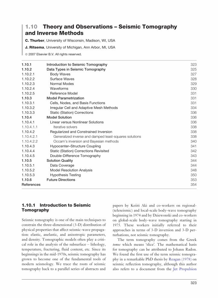
21 May 1998 (Indonesia) at TSUM(H = 28 km; Mw = 6.6; Δ = 101.5°)

Data

PREM synthetic

Body waves

830 1330 1830 2330Time since o

Figure 1 (top) Recorded (vertical component) and (bottom) Pr

seismogram (vertical component) of the 21 May 1998 Indonesia e

body waves and surface waves are indicated.

Section 1.10.5 illustrates how we can evaluate thequality of the model using formal resolution analysesthat invoke an analysis of the properties of the inversematrix G�i, and by forward modeling (hypothesis) tests.We highlight in Section 1.10.6 areas of current andfuture research that are at the forefront of seismictomography. We point out that our discussions areconcentrated on passive-source (i.e., earthquake) tomo-graphy at the crustal through global scale; explorationseismic tomography methods are not covered here.

1.10.2 Data Types in SeismicTomography

In this section, we discuss three general types of data(Figure 1) and their use in the corresponding tomo-graphic methods: body-wave traveltime, surface-wave dispersion, and free-oscillation (normal-mode)spectral measurements. In global tomography, thesethree basic data types provide complementarysampling of the mantle (Figure 2) (see Romanowicz(2003) for a recent review). Teleseismic body-wavetraveltimes are most routinely used in both globaland regional applications. The first global model ofthe deep mantle by Dziewonski et al. (1977) was basedon traveltime picks incorporated in the bulletins ofthe International Seismological Centre (ISC).Subsequent models have utilized the millions of tra-veltime picks the ISC bulletins now comprise (e.g.,Inoue et al., 1990; Vasco et al., 1995; Zhou, 1996; vander Hilst et al., 1997; Bijwaard et al., 1998; Montelliet al., 2004a, 2004b). Global-scale traveltime tomogra-phy has been key in illuminating the variable extentof slab penetration into the lower mantle (e.g., Grand,

rigin (s)2830 3330 3830 4330

Surface waves

eliminary Reference Earth Model (PREM) synthetic

arthquake at station TSUM (Tsumeb, Namibia). The arrival of

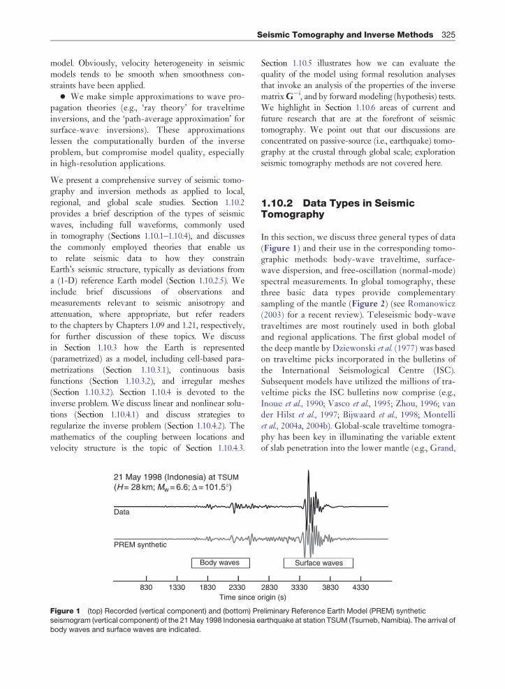
Fundamental-modeRayleigh waves

Teleseismicbody waves

–1.5% +1.5%

Shear velocity variation

120 km 325 km 600 km 1100 km 2100 km

OvertoneRayleigh waves

Figure 2 Maps of shear-velocity variations at 120, 325, 600, 1100, and 2100 km depth. These maps are derived by inverting (top row) fundamental-mode Rayleigh wave,

(middle row) overtone Rayleigh wave, and (bottom row) teleseismic traveltime data. Note that these individual data sets provide complementary structural constraints. Thefundamental modes constrain seismic structure in the upper�300 km of the mantle (depending on the frequency range analysed), the overtone data constrain deeper regions of

the transition zone (less than �1000 km), while teleseismic traveltime data constrain the lower mantle (greater than �1000 km) best.


1994; Grand et al., 1997; Fukao et al., 2001). Surfacewaves generally produce the highest amplitude signalsin seismograms and provide constraints on the uppermantle. Measurements of surface-wave dispersion (i.e.,the frequency-dependent surface-wave speed) are keyin our understanding of lithospheric structure, espe-cially in oceanic regions where few seismic stations arelocated (e.g., Nakanishi and Anderson, 1982; Levequeand Cara, 1985; Nataf et al., 1986; Montagner andTanimoto, 1991; Zhang and Tanimoto, 1993; Laske,1995; Trampert and Woodhouse, 1995; Ekstrom et al.,1997; van Heijst and Woodhouse, 1999). Normal-mode spectral measurements provide constraints onthe longest wavelength part of lateral heterogeneitythrough the Earth (e.g., Masters et al., 1982, 1996; Heand Tromp, 1996; Resovsky and Ritzwoller, 1999).These data lend themselves for joint inversions forshear and compressional velocity (Masters et al.,1996; Deschamps and Trampert, 2004), and even den-sity (Ishii and Tromp, 1999, 2001; Kuo andRomanowicz, 2002). We also briefly discuss the topicsof waveform inversion and the use of reference Earthmodels.

Although several workers have demonstrated thatrobust body-wave (e.g., Bhattacharyya et al., 1996; Reidet al., 2001; Ritsema et al., 2002; Komatitsch et al., 2002;Nolet et al., 2005) and surface-wave (e.g., Romanowicz,1991; Billien et al., 2000; Selby and Woodhouse, 2002;Dalton and Ekstrom, 2006) amplitude patterns can bederived from high-quality data to constrain velocitygradients and attenuation structure, most tomographicstudies of velocity structure are primarily based onwave traveltime or phase delay inversions. Comparedto amplitudes, traveltime data sets possess little scatterand they can be determined in a relatively straightforward manner.

1.10.2.1 Body Waves

Body waves are relatively low-amplitude, impulsivesignals that, at teleseismic distances, propagate alonga variety of paths through the deep mantle and core.Direct waves, surface reflections, and core reflectionsprovide sampling of the mantle along unique paths.In global tomography, teleseismic traveltimes are keyin constraining the structure of the deep mantle.Upper-mantle modeling using teleseismic travel-times and local and regional tomography modelinggenerally rely on measurements from a relativelydense regional network of stations.

Ray theory and Fermat’s principle are at the heartof traditional body-wave traveltime tomography. In

the infinite frequency limit, traveltime T can bewritten as a path integral,

T ¼Z

ray path

uðrÞ ds ½1�

where u is the model of slowness (reciprocal of wavespeed) at points along the ray path, r is position,and ds is an infinitesimal element of path length(see Chapter 1.03). Our problem of determining the3-D slowness structure u(r) from the arrival timeresiduals, obtained by solving a set of equations ofthe general form

dT ¼Z

ray path

duðrÞ ds ½2�

where d represents a perturbation, is confoundedbecause we do not know the true ray path (neglectingfor the moment the additional issues of the hypocen-ter location and origin time if an earthquake is thesource of the arrival). Looked at another way, the raypath used to compute traveltimes from which themodel perturbation is estimated will no longer bethe correct ray path once the perturbations areapplied to the model. Fermat’s principle rescues usfrom this quandary, thanks to the stationary nature oftraveltime under small perturbations to the ray path.Thus, if the path perturbation between the initial andadjusted models is sufficiently small, the traveltime(and therefore the traveltime residual) will be nearlythe same no matter which of the two paths is used.See Snieder (1990), Snieder and Sambridge (1992),and Snieder and Spencer (1993) for a detailed treat-ment of this issue.

It should be clear from eqns [1] and [2] that body-wave traveltime tomography in the infinite fre-quency limit is relatively simple in theory, but morecomplex if finite frequency effects are taken intoaccount in broadband traveltime data analyses. Twosuch examples are ‘fat ray’ tomography (Husen andKissling, 2001) and ‘banana-doughnut’ theory(Dahlen et al., 2000).

Fat ray tomography adopts the view that theentire first Fresnel volume (the volume withinwhich scattered energy arrives within one-half thedominant period of the seismic wave) of the firstarriving phase should be considered in relating tra-veltime residuals to model perturbations. Therefore,the region of the model sensitive to a given datum isbanana shaped for a typically curved path, with thesource and receiver close to (but not at) the tips ofthe banana (Figure 3). Husen and Kissling (2001)

R

TSX + TXR – TSR = T/2

X

S

Figure 3 Diagram of the Fresnel zone for a body wave in

the Earth. A point X is in the first Fresnel zone if the scattered

wave from point X reaches the receiver at R within a timeequal to 1/2 of the wave period T of the direct arrival from

the source S.

328 Seismic Tomography and Inverse Methods

developed such an approach for local earthquaketomography (LET), distributing the contributions toa given traveltime perturbation (eqn [2]) among themodel parameters in proportion to the fraction of the

total Fresnel volume present in a given model cell,rather than along a path of infinitesimal width.

The need for banana-doughnut theory arises whencross-correlation measurements between observed andsynthetic waveforms are used to estimate traveltimes(Dahlen et al., 2000). The seemingly counterintuitiveresult is that the cross-correlation measurement iscompletely insensitive to the model along the geome-trical (infinite frequency) ray path, producing a hole

within the banana along the ray path – hence the termbanana doughnut. As one might expect, the volume ofthe banana and its interior ‘hole’ are strongly frequencydependent. However, whether finite-frequency effectsimpact the resolution of Earth structure is still a matter

of debate (Montelli et al., 2004a, 2004b; van der Hilstand De Hoop, 2005).

Another source of complexity is anisotropy, wherewavespeed depends on the direction of wave propa-

gation or wave polarization. For shear waves,anisotropy is most readily identified via shear-wavesplitting (SWS; an example of birefringence) (e.g.,Silver, 1996). A shear wave with an initial linearpolarization will be ‘split’ as it passes through an

anisotropic zone (when the initial polarization direc-tion is not aligned with an axis of the anisotropicstructure). Therefore, fast shear-wave polarizationdirections and splitting times can readily be mea-sured. However, it is not straightforward to model

SWS, at least in a tomographic sense. In contrast,P-wave anisotropy is not directly observable in asingle three-component seismogram. P waves simplycannot be ‘split’ in the same manner transverseS waves can. Instead, P-wave traveltimes throughan anisotropic volume depend on propagation direc-tion, making it difficult to separate P-waveanisotropy from P-wave-speed heterogeneity,although a tomographic modeling approach is stillpossible (Hirahara, 1993). The use of SWS observa-tions to provide a priori constraints for an anisotropicP-wave tomographic inversion is one practicalapproach (Eberhart-Phillips and Henderson, 2004).See Chapter 1.09 for a thorough discussion of seismicanisotropy.

Attenuation, on the other hand, can be approachedreadily in the same manner for P and S waves. Even ifthe quality factor Q (Aki and Richards, 1980) isfrequency independent, higher-frequency wavesundergo greater intrinsic attenuation than low-fre-quency waves because they pass through more wavecycles. Their amplitude decays exponentially:

Aðx; f Þ ¼ A0 exp –�fx

VQ

� �� ½3�

where V is wavespeed, f is frequency, and x is dis-tance of propagation. A common approach fortomography is to express attenuation in terms of theparameter t � (defined as traveltime/quality factor),leading to an integral relationship between t � and Q

along the path,

t � ¼Z

path

dt

Q ðrÞ ¼Z

path

ds

V ðrÞQ ðrÞ ½4�

t � values at a set of observing stations for a givenearthquake can be determined by joint, nonlinearfitting of observed spectra using an accepted sourcemodel (Lees and Lindley, 1994). The t� values canthen be inverted for a 3-D Q model in a mannerequivalent to body-wave tomography (Scherbaum,1990; Rietbrock, 2001). See Chapter 1.21 for a moregeneral discussion of attenuation.

1.10.2.2 Surface Waves

There are two types of surface waves with differentparticle motion characteristics, just as there aretwo types of body waves – but with a ‘twist’.Surface waves are evanescent waves (with a purelyimaginary vertical wave number ijvj) that propagatehorizontally along the Earth’s surface with a ‘skin


depth’ that increases with increasing period (or wave-

length). Love waves are composed of horizontallypolarized shear waves (SH) trapped within a surface

layer (or layers). Rayleigh waves form byan interaction between compressional and vertically

polarized shear waves (P-SV) at the surface. The

combination of the Earth’s sphericity and theincrease of wavespeed with depth leads to dispersion

of surface waves. As a result, surface waves are

recorded as a ‘train’ of waves, with long-period/long-wavelength waves generally arriving first. At

teleseismic distances, surface waves have much largeramplitude than body waves due to their geometric

spreading in 2-D, as opposed to the 3-D spreading of

body waves.One consequence of dispersion is the existence of

two distinct velocities characterizing surface-wave

propagation. Let us express displacement u (x, t)

as an integral over harmonic plane waves of all fre-quencies o :

uðx; tÞ ¼Z

Að!Þ expfið!t – kð!ÞÞx þ �ð!Þg d! ½5�

If we approximate the wave number k (o) by aTaylor series about o0,

kð!Þ ¼ kð!0Þ þ ðdk=d!jð! ¼ !0Þð! – !0Þ ½6�

it is straightforward to show that the displacementdue to harmonic waves near o0 is approximately

uðx; tÞ ¼Z !0þd!

!0 – d!

Að!Þ expfið! – !0Þðt – dk=d!xÞg

� expfið!0t – kð!0ÞxÞ þ �Þg d! ½7�

The two sinusoidal functions in [7] correspond topropagating waves with different speeds. The carrierwave at frequency o propagates at the phase velocity(C) o0/k, upon which a more slowly varying envel-ope with frequency do and wave number dk issuperposed. This envelope propagates at the groupvelocity (U) do/dk.

Surface-wave group velocity analysis involvesmultitapered spectral analysis of narrow-band fil-

tered signals,

sðtÞ ¼Z

sð!ÞHð!Þ d! ½8�

where H(o) is the taper function, usually of the formexp{�(o�o0)2/o0

2}. Group velocity can be deter-mined by estimating how the peak of the amplitudespectrum varies as a function of group velocityU (¼epicentral distance/traveltime) and the central

frequency of the taper function. This analysis hasbeen applied globally to determine group velocitydispersion (see Chapters 1.01 and 1.02).

Phase velocities are determined either with datafrom multiple stations, or from single seismograms.The phase �i (determined from the Fourier trans-form) of a recording i at a distance xi can be written as

�i ¼!t – kð!Þxi þ �s þ 2n�

¼!½t – x=cð!Þ�þ �s þ 2n� ½9�

where �s is the initial phase (due to the source).Defining �ij as �i – �j for stations i and j at the sameazimuth from the source (so that �s is common to bothrecordings i and j ), we can solve for the phase velocity

Cð!Þ ¼ !ðxi – xj Þ=½!ðti – tj Þ þ 2ðm – nÞ� –�ij � ½10�

The term 2(m – n)� is found empirically by ensuringthat the phase velocity has a ‘reasonable’ value at thelongest periods. The subsequent analysis at increas-ingly shorter periods is ‘locked in’ by requiring that C

is a continuous function of o.Single-station (i ) measurements of phase velocity

require knowledge of �s(o), that is, knowledge of theearthquake focal mechanism:

Cð!Þ ¼ !x=½!t þ �sð!Þ þ 2n� – �i � ½11�

Often, we measure the phase �(o) relative to that ina synthetic seismogram for a spherically symmetricEarth model ��¼�obs��syn. Again, we removethe ‘cycle-skip’ ambiguity by locking 2n� at thelowest frequencies, and estimating �� at increas-ingly higher frequencies. For further details, see

Chapters 1.01, 1.02, and 1.05.

1.10.2.3 Normal Modes

Normal modes (also known as ‘free oscillations’) arestanding waves excited by the largest earthquakes onEarth. Like standing waves on a string fixed at bothends, normal modes have distinct frequencies deter-mined by Earth’s finite size and its internal elasticstructure. The gravest normal mode, the so-called‘football mode’, has a period of about 54 min. Inanalogy to surface waves (intimately related to nor-mal modes), there are two types of normal modes,distinguished by their mode of oscillations. Torsionalmodes are analogous to Love waves. They do nothave radial displacements and they do not causevolume changes. Spheroidal modes are analogous toRayleigh waves, and involve a combination of radialand transverse motions. Like standing waves on a


string, we can express the displacement field in theEarth as a sum of normal modes (e.g., Gilbert, 1970;Dahlen and Tromp, 1998):

uðx; tÞ ¼X

n

Xl

X1

m¼ – 1

nAml ð!ÞnYl ðrÞXm

l ð�; �Þ

� expfi!ml tg ½12�

Each mode is described by its radial order n, andsurface order l and m. These integers describe thefrequency nol

m of the normal mode, and the spatialshape of the radial eigenfunction nYl (r) and surfaceeigenfunction Xl

m(�, �). A sum of normal modesdescribes the complete wavefield up to frequencyol

m. However, due to the computational burden, nor-mal modes are used to study primarily long period(T > 20–50 s) wave propagation in practice.

A ‘multiplet’ nol consists of 2lþ 1 ‘singlets’ nolm

(m takes values between –l andþl ). For a sphericallysymmetric Earth, the singlet eigenfrequencies are thesame. For a laterally heterogeneous Earth, the multi-plet ‘splits’, rendering singlets nol

m with slightlydifferent eigenfrequencies. Earth’s rotation has anobservable effect on the gravest multiplets (e.g., 0S2

and 0S3). Lateral heterogeneity (both elastic hetero-geneity and anisotropy) can cause even moresplitting. Tomographers use observations of splittingto constrain the large-scale variations (e.g., Giardiniet al., 1987; Masters et al., 1996; Ishii and Tromp,1999; Resovsky and Ritzwoller, 1999), albeit thatonly the ‘even-degree’ structure can be constrainedin a direct manner.

It is difficult to make splitting measurements.Spectral peaks have a finite width, because seismo-grams are not infinitely long, and due to the effect ofanelasticity. Moreover, multiplets can overlap, whichmakes it impossible to treat them in isolation.However, analysis of the splitting of coupled multi-plets enables us to constrain both even-degree andodd-degree structure (Dahlen and Tromp, 1998). See

Chapters 1.01, 1.02, and 1.05 for further details.

1.10.2.4 Waveforms

While traveltimes and phase delays represent para-metric measurements made from seismograms, it isalso possible to model the seismograms directly ‘wig-gle for wiggle’. Waveform inversions are particularlyadvantageous in that it allows for the analysis ofstrongly interfering signals. A waveform inversion istypically posed as a search for the model m that best

minimizes the (least-squares) fit between theobserved seismogram (or a segment of it) d(t) and a

computed seismogram s (m, t):

FðmÞ ¼Z

dtfdðtÞ – sðm; tÞg2 ½13�

In global tomography, waveform fitting was intro-duced by Woodhouse and Dziewonski (1984) using

digital seismic data from upgraded global seismicstations. An important novelty of their approach is

that it allows for the recovery of both even and odd

spherical harmonic coefficients. In their approach,still widely used today, synthetic seismograms were

computed using normal mode summation. The ‘path-average approximation’ accounts for the effects of

lateral heterogeneity by perturbing the eigenfre-quency of each multiplet. Using eqn [12] as a

description of a long-period seismogram, we canfind perturbations to d�(r), d�(r), and d�(r) due to

perturbations in frequency do. We can write thedependence of do(�, j) as

d! ¼Z

gc

ðK� d�þ K� d� þ K� d�Þ dS ½14�

where the 1-D kernels K�, K�, and K� describe thedependence of perturbation in eigenfrequency o toperturbations in P velocity, S velocity, and density,respectively (see Dahlen and Tromp (1998) for anextensive theoretical treatment).

The ‘partitioned waveform inversion technique’(Nolet and Snieder, 1990) also utilizes the path-aver-

age approximation approach, but given its focus onsmaller (continental-scale) regions (e.g., Zielhuis and

Nolet, 1994; van der Lee and Nolet, 1997; Lebedevet al., 1997), it is limited to minor-arc waveforms only

albeit at somewhat higher frequencies. The methodenables the separate analysis (and data weighing) of

fundamental-mode surface waves and overtone sig-nals (such as triplicated SS, SSS waves) and

background seismic models unique to different pro-pagation paths.

More recent work has focused on the develop-ment of more realistic kernels. Two-dimensional

kernels computed using across-branch coupling(e.g., Li and Tanimoto, 1993; Li and Romanowicz,

1995; Marquering and Snieder, 1995; Zhao andJordan, 1998) include (frequency-dependent) sensi-

tivity along the body-wave propagation pathwithin the plane of propagation. These higher-order

(compared to the path-averaged approximation byWoodhouse and Dziewonski (1984)) kernels, better


describe the sensitivity of overtone surface waves and

complex body waves like SS (the surface reflected S

wave) and Sdiff (the core-diffracted S wave) to Earth

structure. Models SAW12D (Li and Romanowicz,

1996) and SAW24B16 (Megnin and Romanowicz,

2000) are based on these 2-D kernels.At a regional scale, Zhao et al. (2005) demonstrated

the ability to compute the Frechet kernels for the full-

waveform inverse problem using a 3-D starting model,

opening up the avenue of iterative waveform tomo-

graphy at regional scales. The data are frequency-

dependent phase delay and amplitude anomalies

(Gee and Jordan, 1992), which are evaluated using

cross correlation between the observed data and syn-

thetics. Chen et al. (2007) applied this approach to the

Los Angeles region, leading to improvements in exist-

ing models of 3-D structure based on traveltime

tomography and active-source models.

1.10.2.5 Reference Model

A radially symmetric (1-D) model of wave speed

takes a central role in the analysis of global seismic

data and global tomography. The Jeffreys Bullen

Tables ( Jeffrey and Bullen, 1958), 1066A (Gilbert

and Dziewonski, 1975), Preliminary Reference

Earth Model (PREM; Dziewonski and Anderson,

1981), IASP91 (Kennett and Engdahl, 1991), and

ak135 (Kennett et al., 1995) are often invoked. They

provide wave speed or a combination of wave speed,

density, and attenuation as a function of depth in the

Earth, and explain to first order the characteristics of

global wave propagation, such as the propagation

time of teleseismic body waves, and the dispersion

of surface waves (including in some cases the effect of

upper-mantle anisotropy). Using digital broadband

recordings, tomographers have built catalogs of sur-

face-wave dispersion measurements (e.g., Ekstrom

et al., 1997; Trampert and Woodhouse, 1996) and

catalogs of body-wave traveltimes (e.g., Woodward

and Masters, 1991; Su et al., 1994; Ritsema et al., 2002)

by systematically comparing recorded and PREM

synthetic waveforms (Figure 1).The 1-D reference model is also used in the for-

ward modeling theory. For example, a body-wave

traveltime anomaly, dT, can be defined in terms of

velocity as (see Section 1.10.2.1)

dT �Z

s0

1

V02 ðrÞ dV ðrÞ ds ½15�

Similarly, a surface-wave phase-velocity perturba-tion dC(o) due to shear velocity heterogeneity inthe mantle can be written as

dCð!Þ ¼Z

gc

ds

Zdr

qCð!ÞqV 0

S ðrÞ

� �dVSðrÞ ½16�

where we have assumed that surface waves propagatealong the great circle path gc and that the relationshipbetween phase velocity C and shear velocity VS can becalculated for the 1-D reference model. It is straight-forward to compute 1-D synthetics, body-wave paths,and kernel functions that relate surface-wavedispersion to seismic velocity for 1-D seismicmodels. Moreover, eqns [15] and [16] render linearrelationships between the seismic observables andwave speed heterogeneity. These can be solved usingstandard linear inverse techniques (see Section 1.10.4).Current research addresses how better, but morecomplex, theories affect the model solution.

In local-scale studies, the importance of the starting1-D model has been clearly demonstrated. For exam-ple, Kissling et al. (1994) proposed the use of the‘minimum 1-D model’ determined by inversion for alayered structure as the starting model for 3-D tomo-graphy. Refraction models provide another potentialsource for a starting 1-D model. Because the LETproblem is strongly nonlinear, a suitable startingmodel is critical for reaching an optimal solution.

1.10.3 Model Parametrization

The Earth’s seismic velocity structure has been repre-sented in a wide variety of ways in seismic tomographystudies. All are only approximations to the true 3-Dstructure of the Earth, or some portion of it. The Earthhas heterogeneous structure on a vast range of spatialscales, including complications such as discontinuities,faults, layering, intrusions, inclusions, zones of elevatedtemperature or partial melt, and random geologic het-erogeneities. It also displays anisotropy, which is thetopic of Chapter 1.09. The spatial scale of heterogene-ity that can be imaged with seismic tomographydepends primarily on the density of wave sampling,with a lower bound proportional to the minimumwavelength of recorded seismic-wave energy.

1.10.3.1 Cells, Nodes, and Basis Functions

No single scheme can fully represent all aspects ofthe Earth’s heterogeneity. At the local scale, the


constant-velocity, uniform volume block approach ofAki and Lee (1976) and the variable volume blockapproach of Roecker (1982) treat a volume of theEarth as a set of cells within each of which the seismicvelocity is constant (Figure 4(a)). This approach hasthe advantage of simplicity, but is clearly lacking inthe ability to represent heterogeneous structurefaithfully, even structures as simple as slight gradi-ents in velocity or oblique discontinuities. From theinverse theory point of view, a block/cell inversion isoften set up as an overdetermined problem (moreindependent data than unknowns), but this strategycan be criticized for being underparametrized (insuf-ficient parameters to adequately represent the realEarth). At the same time, some model parametersmay actually be unconstrained even though thereare more data than unknowns, resulting in a mixed-determined problem (simultaneously over- andunderdetermined). Alternatively, one can employ alarge number of small cells, allowing gradual or rapidvelocity changes from block to block to mimic gra-dients or discontinuities, respectively (Nakanishi,1985; Walck and Clayton, 1987; Lees and Crosson,1989). Unfortunately, the use of a large number of

(a) (b)

(d)(

CoM

P

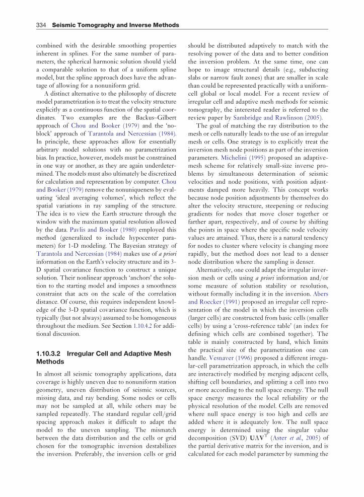
Figure 4 Examples of types of model parametrization scheme

laterally varying but vertically constant velocity within a given laycells. (e) Interfaces separating regions with velocity defined on a gr

(1992) Tomographic imaging of P and S wave velocity structure

Research 97: 19909–19928, with permission from American Geo

cells, if not compensated for, results in a severelyunderdetermined problem (many more unknownsthan independent data), and increased computationalburden. These two problems are typically dealt withby applying a smoothing operator and a sparse-matrix solver, respectively (see Section 1.10.4).

Variations on the discrete block parametrizationinclude laterally varying layers (Hawley et al., 1981)and a 3-D grid of nodes (Thurber, 1983). In theapproach of Hawley et al. (1981), the model is dividedinto horizontal layers in which velocity is constant inthe vertical direction, but velocity is obtained byinterpolation in the horizontal directions among ver-tical nodal lines (Figure 4(b)). The spacing betweennodal lines may vary from layer to layer. Thurber(1983) used a 3-D grid approach (Figure 4(c)), inwhich velocity varies continuously in all directions,with linear B-spline interpolation among nodes.Alternatively, one can use cubic B-splines with con-tinuous second-order derivatives (Michelini andMcEvilly, 1991).

Another variant of the 3-D grid theme is to con-sider each set of four neighboring nodes as definingthe vertices of a tetrahedron (Figure 4(d); Lin and

(c)

e) Anradoho

late boundary

BSurface

s. (a) Constant-velocity, uniform volume blocks. (b) Layers of

er. (c) Regular grid of nodes. (d) Variable-size tetrahedralid. (e) Reproduced from Zhao D, Hasegawa A, and Horiuchi S

beneath northeastern Japan. Journal of Geophysical

physical Union.


Roecker, 1997). The four node velocities can be usedto define a unique linearly varying velocity fieldwithin the tetrahedron; the velocity gradient canthus point in any direction. Snell’s law is used tocross tetrahedron boundaries. This allows the use ananalytic formula for ray tracing using an initial-value(‘shooting’) approach, as ray paths are circulararc segments in a medium with constant-velocitygradient. Other alternative interpolation schemesare possible, but would require different ray-tracingprocedures. See also Section 1.10.3.2 for an exampleof the use of tetrahedrons in adaptive-meshtomography.

Similar approaches have been adopted for regio-nal- and global-scale tomography. Aki et al. (1977)employed constant-slowness, uniform volume cellsin their original teleseismic (regional) inversionwork, and that method (ACH after the authors Aki,Christoffersson, and Husebye) has proven to be a‘workhorse’ for the seismology community (seeEvans and Achauer, 1993). Some improvementshave been made to the algorithm over the years,including allowing for variable block thickness withdepth (Evans and Achauer, 1993) and using nodeswith spline interpolation (VanDecar et al., 1995), andproblems and code errors have been pointed out(Masson and Trampert, 1997; Julian et al., 2000), butthe basic method continues to be used widely.Humphreys and co-workers developed a similaralgorithm (Humphreys et al., 1984), and Spakman,Nolet, and co-workers developed a third comparablealgorithm (Spakman and Nolet, 1988), both of whichhave also been put to wide use. A key distinctionbetween the latter two is the inverse problem solu-tion method, SIRT for the former and LSQR for thelatter (see Section 1.10.4).

Zhao and co-workers have taken a slightly differ-ent approach that emphasizes the importance ofmajor seismic velocity discontinuities along withvelocity heterogeneity. Using the study of northeast-ern Japan by Zhao et al. (1992) as an example, theauthors define the discontinuities and embed a velo-city grid within each layer (Figure 4(e)). Themethod allows the inclusion of secondary phasedata (e.g., converted phases) to model the positionsof the discontinuities, although this particular studydid not utilize this capability.

Similarly, Zhao (2004) incorporated discontinu-ities and a 3-D grid in a global tomographic model,with a grid spacing of 3–5�. Specifically, he includedthe Moho and the 410 and 660 km discontinuities,keeping them fixed during the inversion. More

commonly, global tomographic models utilize sphe-rical ‘blocks’ of uniform latitude and longitude extentor roughly uniform size (Sengupta and Toksoz, 1976;Inoue et al., 1990; Vasco et al., 1995; Zhou, 1996; vander Hilst et al., 1997).

Alternatively, one can adopt a functionalapproach to representing 3-D structure, either witha set of basis functions or an a priori functional form.An example of the former is an expansion in a set ofcontinuous, orthogonal basis functions (e.g., sinusoi-dal or spherical harmonic functions) where thespatial resolution is limited by the number of termsincluded in the expansion (Novotny, 1981).Examples of the latter are the subducting slab para-metrization of Spencer and Gubbins (1980), in whichthe slab is represented by its strike, dip, width, slow-ness contrast, and decay rate with depth; the faultzone parametrization of Wesson (1971), in which thefault zone is represented by its velocity decrease,decay with depth and distance, and the velocity con-trast across it; and the quasi-layered parametrizationof Ashiya et al. (1987) employing a sum of hyperbolictangent functions for the depth variation of velocityand Chebyshev functions for the lateral variation ofvelocity.

Early global P-wave traveltime studies used sphe-rical-harmonic expansions in latitude and longitudeand polynomials in depth (Dziewonski, 1984). Arecent example of these studies reached degree 40,corresponding to a lateral dimension of as little as500 km (Boschi and Dziewonski, 1999). One source ofconcern for this approach is the tendency for thetruncated basis functions to leak into the solution,leading to a biased model estimate (Trampert andSnieder, 1996). If the power in the model spectrumabove the truncation point is weak, this may not be aserious issue, but of course it is difficult to prove thisis the case, in general. We also point out that trunca-tion is a risk to virtually any tomographic methodthat adopts an overdetermined (‘underparametrized’)inverse approach. Trampert and Snieder (1996) infact present a technique for correcting (to firstorder) the biasing effect of truncating spherical har-monic basis functions.

Recently, cubic splines have been used for globaltomography (Antolik et al., 2000; Megnin andRomanowicz, 2000). Spherical splines (Wang andDahlen, 1995) are used for the horizontal variationsand radial splines for the vertical. This approach hasthe advantage of being a local parametrization, lead-ing to a sparse solution matrix and potentiallyavoiding the bias problems of spherical harmonics,


combined with the desirable smoothing propertiesinherent in splines. For the same number of para-meters, the spherical harmonic solution should yielda comparable solution to that of a uniform splinemodel, but the spline approach does have the advan-tage of allowing for a nonuniform grid.

A distinct alternative to the philosophy of discretemodel parametrization is to treat the velocity structureexplicitly as a continuous function of the spatial coor-dinates. Two examples are the Backus–Gilbertapproach of Chou and Booker (1979) and the ‘no-block’ approach of Tarantola and Nercessian (1984).In principle, these approaches allow for essentiallyarbitrary model solutions with no parametrizationbias. In practice, however, models must be constrainedin one way or another, as they are again underdeter-mined. The models must also ultimately be discretizedfor calculation and representation by computer. Chouand Booker (1979) remove the nonuniqueness by eval-uating ‘ideal averaging volumes’, which reflect thespatial variations in ray sampling of the structure.The idea is to view the Earth structure through thewindow with the maximum spatial resolution allowedby the data. Pavlis and Booker (1980) employed thismethod (generalized to include hypocenter para-meters) for 1-D modeling. The Bayesian strategy ofTarantola and Nercessian (1984) makes use of a priori

information on the Earth’s velocity structure and its 3-D spatial covariance function to construct a uniquesolution. Their nonlinear approach ‘anchors’ the solu-tion to the starting model and imposes a smoothnessconstraint that acts on the scale of the correlationdistance. Of course, this requires independent knowl-edge of the 3-D spatial covariance function, which istypically (but not always) assumed to be homogeneousthroughout the medium. See Section 1.10.4.2 for addi-tional discussion.

1.10.3.2 Irregular Cell and Adaptive MeshMethods

In almost all seismic tomography applications, datacoverage is highly uneven due to nonuniform stationgeometry, uneven distribution of seismic sources,missing data, and ray bending. Some nodes or cellsmay not be sampled at all, while others may besampled repeatedly. The standard regular cell/gridspacing approach makes it difficult to adapt themodel to the uneven sampling. The mismatchbetween the data distribution and the cells or gridchosen for the tomographic inversion destabilizesthe inversion. Preferably, the inversion cells or grid

should be distributed adaptively to match with theresolving power of the data and to better conditionthe inversion problem. At the same time, one canhope to image structural details (e.g., subductingslabs or narrow fault zones) that are smaller in scalethan could be represented practically with a uniform-cell global or local model. For a recent review ofirregular cell and adaptive mesh methods for seismictomography, the interested reader is referred to thereview paper by Sambridge and Rawlinson (2005).

The goal of matching the ray distribution to themesh or cells naturally leads to the use of an irregularmesh or cells. One strategy is to explicitly treat theinversion mesh node positions as part of the inversionparameters. Michelini (1995) proposed an adaptive-mesh scheme for relatively small-size inverse pro-blems by simultaneous determination of seismicvelocities and node positions, with position adjust-ments damped more heavily. This concept worksbecause node position adjustments by themselves doalter the velocity structure, steepening or reducinggradients for nodes that move closer together orfarther apart, respectively, and of course by shiftingthe points in space where the specific node velocityvalues are attained. Thus, there is a natural tendencyfor nodes to cluster where velocity is changing morerapidly, but the method does not lead to a densernode distribution where the sampling is denser.

Alternatively, one could adapt the irregular inver-sion mesh or cells using a priori information and/orsome measure of solution stability or resolution,without formally including it in the inversion. Abersand Roecker (1991) proposed an irregular cell repre-sentation of the model in which the inversion cells(larger cells) are constructed from basic cells (smallercells) by using a ‘cross-reference table’ (an index fordefining which cells are combined together). Thetable is mainly constructed by hand, which limitsthe practical size of the parametrization one canhandle. Vesnaver (1996) proposed a different irregu-lar-cell parametrization approach, in which the cellsare interactively modified by merging adjacent cells,shifting cell boundaries, and splitting a cell into twoor more according to the null space energy. The nullspace energy measures the local reliability or thephysical resolution of the model. Cells are removedwhere null space energy is too high and cells areadded where it is adequately low. The null spaceenergy is determined using the singular valuedecomposition (SVD) U�VT (Aster et al., 2005) ofthe partial derivative matrix for the inversion, and iscalculated for each model parameter by summing the


squares of the elements of the row of the orthogonalmatrix V corresponding to the given model para-meter for singular values below a chosen threshold.This process is extremely time consuming for large-scale problems, as it is not fully automatic.

In contrast, for LET, Zhang and Thurber (2005)developed an automatic adaptive-mesh tomographymethod based on tetrahedral cells that matches theinversion mesh to the data distribution. As a result,the number of inversion mesh nodes is greatlyreduced compared to a regular inversion grid withcomparable spatial resolution, and the tomographicsystem is more stable and better conditioned. Theystart the inversion from a slightly perturbed regularinversion grid, constructing the tetrahedral cells (oralternatively the Voronoi diagram) around the nodesusing the Quickhull algorithm (Barber et al., 1996).Rays are traced between events and stations based onthe current regular velocity grid. The rays are used tofind the partial derivatives of the traveltimes withrespect to the model slowness parameters on thecurrent inversion mesh. In the process, the values ofthe ‘derivative weight sum’ (DWS – the sum of theinterpolation weights for the partial derivatives cor-responding to each model parameter; Thurber andEberhart-Phillips, 1999) for the inversion mesh nodesare calculated. Threshold DWS values are set foradding or removing nodes. Once the inversion meshis determined to be optimal, a new set of tetrahedralcells (or new Voronoi diagram) is constructed, andthe partial derivatives of the traveltimes with respectto the new set of inversion mesh nodes are calculated.Following each simultaneous inversion, the velocityvalues on the irregular inversion mesh nodes areupdated, rays are traced through the new model,and the inversion mesh is again updated followingthe same procedure to assure a good match with theray distribution, which will change as the velocitymodel changes and hypocenters move. Compared tothe above methods, key advantages of this approachare that it is fully automatic and it uses the samplingdensity to control the mesh density.

A variety of irregular cell and adaptive mesh tech-niques have also been developed for whole-Earthtomography. One simple approach is the use of twocell sizes, a larger cell for a ‘background’ global 3-Dmodel plus a smaller cell size in a region of interest(Widiyantoro and van der Hilst, 1997). In a similar butmore versatile vein, Spakman and Bijwaard (2001)followed the basic idea of Abers and Roecker (1991)discussed above, but adopted a different strategy forirregular cell design by developing a completely

automated and fast algorithm for the construction ofthe cross-reference table. The design of irregularcells can be constrained by some scalar function, forinstance a measure of model sampling such as cellhit count.

Sambridge and Gudmundsson (1998) proposed anirregular cell approach for global tomography basedon tetrahedral diagrams. Their initial application wasto a regionalized model using a priori information ontectonic provinces and subducting slab geometry toconstruct a fixed-grid model (Gudmundsson andSambridge, 1998), but they did not explicitly explainhow to optimize the cells. Some possibilities are toadjust them based on the model null space energy(Vesnaver, 1996) and/or the velocity gradient. Morerecently, Sambridge and Faletic (2003) introduced adata-driven tetrahedral cell adaptive scheme basedon the maximum spatial gradients in seismic velocityperturbation across each tetrahedron face. This isuseful for trying to characterize regions of rapidvelocity change, but it does not account for the abilityof the data to resolve such changes. Nolet andMontelli (2005) took a similar tetrahedral parametri-zation approach, but included an estimate of localresolving length in deriving the optimal spacing ofmesh nodes.

It is clear that there are many options available formodel parametrization. How does one make achoice? One approach that has some advantages isto adopt a two-stage modeling strategy. An initialphase of modeling can be carried out using a more‘traditional’ regular parametrization. The results ofthe first phase can then serve as both starting modeland point of comparison for a second phase usingsome type of irregular model parametrization. Anysignificant increase in anomaly amplitudes should beaccompanied by a significant decrease in data misfit(e.g., as measured by an F-test) if the results of thesecond phase are to be preferred over the first. Theirregular parametrization also is a hindrance to car-rying out some of the traditional resolution tests,such as spike or checkerboard tests (see Section1.10.5.2). Such resolution tests from the regular para-metrization model can provide valuable informationthat might not easily be obtained otherwise. At thesame time, there is potential concern about the modelresolution for models with locally fine parametriza-tion – unless a complete resolution analysis is carriedout, the reality of fine-scale features resulting fromirregular mesh tomography may be questioned. SeeSections 1.10.4 and 1.10.5 for detailed discussion ofmodel resolution issues.


1.10.3.3 Static (Station) Corrections

In many cases, the adopted model parametrization isstill incapable of representing some aspect or scale ofEarth heterogeneity. The most common situation istreating the shallow structure (e.g., the top few hun-dred meters at a local scale, or the crust at the globalscale) using static (station) corrections. These correc-tions can be defined a priori or determined as part ofthe inversion. The mathematics of the latter optionare treated in Section 1.10.4 below; examples includeBijwaard et al. (1998) and Li and Romanowicz (1996)for global and DeShon et al. (2006) for local body-wave tomography. Examples of the a priori approachinclude using time and phase delays computed from aglobal crustal model (Nataf and Ricard, 1996;Mooney et al., 1998) in global or regional surface-wave tomography (Montagner and Tanimoto, 1991;Boschi and Ekstrom, 2002; Boschi et al., 2004), orusing a fixed crustal refraction model in teleseismictomography (Waldhauser et al., 2002). In all of thesecases, the goal is to prevent shallow heterogeneityfrom ‘leaking’ into the deeper structure. The effec-tiveness of this strategy obviously hinges on thequality of the a priori or derived correction valuesand on how well the highly nonlinear effects of stronglateral variation in crustal structure are dealt with.Recognizing this, Li et al. (2006) adopted a strategyfor teleseismic tomography that allows for perturba-tions to the a priori crustal model by including aregularization term in the inversion that penalizesdeviations from the a priori model. Thus, the crustalmodel will be perturbed where the data require it,although the penalization will generally moderatesuch changes.

1.10.4 Model Solution

In the early days, the limited computer capabilities(typical mainframes with a megabyte of memory, 100MB of disk space, and megahertz CPU speeds) putsevere limits on the mathematical and computationalsophistication that could be implemented for solvingtomography problems. Now we have inexpensivedesktop systems with 3 orders of magnitude largermemory and storage and faster speed than themainframes of the mid-1970s, yet tomographerswill still complain that their computers are too slowand their memory and storage capabilities are notadequate! As computer power has increased, theamount of data and the complexity of both the

model parametrization and the associated forwardproblem solver have risen as well.

The preceding sections set the stage for the criti-cal process of determining a model that adequatelyfits the available data and known constraints. To getto this point, the tomographer needs to make numer-ous decisions regarding the scale of the problem to betackled, the types of data to include, the manner inwhich the 3-D Earth structure will be represented,how the forward modeling will be carried out, etc.Deriving an ‘optimal’ model and evaluating its qual-ity falls under the domain of inverse theory, aboutwhich numerous books have been written (Menke,1989; Parker, 1994; Aster et al., 2005; Tarantola, 2005).A series of papers by Backus and Gilbert (1967, 1968,1970) can be credited with bringing linear inversetheory to the attention of geophysicists, and Wiggins(1972) wrote a noteworthy paper on resolution ofseismic models in particular. While we do not havespace to review all the fundamental aspects of inversetheory as they can be applied to seismic tomography,we can provide a ‘road map’ to guide the appropriateapplication of inverse methods to tomographyproblems.

1.10.4.1 Linear versus Nonlinear Solutions

One key aspect that separates some tomography pro-blems from others is whether the problem is linear ornonlinear. For example, fitting a straight line to a setof x–y points is a linear problem, as is fitting a para-bola. In the former case, the equations are of the form

y ¼ ð1Þm1 þ ðxÞm2 ½17�

whereas in the latter case, they are of the form

y ¼ ð1Þm1 þ ðxÞm2 þ ðx2Þm3 ½18�

Both can be expressed directly in the form

d ¼ Gm ½19�

where d is the data vector of length N, m is a vectorwith M model parameters, and G is the matrix ofpartial derivatives of the data with respect to themodel parameters. In contrast, fitting a Gaussiancurve to a set of x–y points is a nonlinear problem,because the formula

y ¼ m1=½ð2�Þ1=2m2� exp½ – ðx –m3Þ2=ð2m2

2 Þ ½20�

cannot be reduced to a linear equation in terms ofthe variables mi. We point out that solving nonlinearproblems in seismic tomography is generally


accomplished via linearizing the problem about atrial solution and improving the model iteratively(see Aster et al., 2005). The few exceptions applyglobal optimization methods such as Monte Carlo(Shapiro and Ritzwoller, 2002), but that is beyondthe scope of this chapter.

To some degree, this distinction is fuzzy for tomo-graphy problems because the same problem can betackled with either a linear or nonlinear approach.Take, for example, the original LET study of Aki andLee (1976). In a single step, they inverted simulta-neously for local earthquake locations and 3-Dstructure (in terms of constant-slowness ‘blocks’)using a homogeneous background velocity model.They explored the linearity of the problem andmodel uniqueness by repeating the inversion withtwo different background models. Given the conver-gence to the same 3-D structure, they concluded thata linear solution was adequate. Subsequent work onan expanded data set from the same region demon-strated that a nonlinear solution actually wasrequired to converge to a valid solution. In thiscase, the lateral heterogeneity was so strong that thelinear inversion had not converged. Starting with thestudy of Thurber (1983), nonlinear solutions havebecome the norm for LET.

Similarly, the original ACH (Aki et al., 1977) tele-seismic tomography study used a linear inversion.Work by Ellsworth (1977) determined that a nonlinearsolution agreed well with the linear solution for a dataset from Hawaii. In this case, however, the amplitudeof the anomalies was relatively modest (mainly within5%), so a linear approximation was in fact adequate.For regions with higher amplitude anomalies, a non-linear solution could be significantly different. Earlyefforts at nonlinear teleseismic inversion were madeby Thomson and Gubbins (1982), Koch (1985), andNakanishi and Yamaguchi (1986). More recently,Weiland et al. (1995) and VanDecar et al. (1995) devel-oped nonlinear algorithms for teleseismic tomographyand applied them to Long Valley caldera, CA, andeastern Brazil, respectively. In the case of Long Valley,anomalies on the order of 20% were recovered,about 3 times larger than a linear inversion byDawson et al. (1990) using the same data set. A similarstudy for Valles Caldera, New Mexico (Steck et al.,1998), obtained even greater anomalies (25%) usingnonlinear inversion. Despite such impressive resultswith a nonlinear approach, linear inversions are pre-dominant in teleseismic tomography studies.

On a global scale, linear solutions are also thenorm for traveltime inversions, whether they are

block or spline inversions or spherical harmonicexpansion inversions. Beginning with Sengupta andToksoz (1976) and Dziewonski et al. (1977) and con-tinuing through Su et al. (1994) and van der Hilst et al.(1997) (and many others), the inverse problems weremainly set up and solved in a linear manner. Somenotable exceptions are the P-wave study of Bijwaardand Spakman (2000) and the S-wave study ofWidiyantoro et al. (2000), which are both fully non-linear solutions. We also note that Dziewonski (1984)also carried out an iterative inversion but with anapproximate inverse that neglected hypocenter–structure coupling (see Section 1.10.4.3).

Using a 3-D ray tracer (Bijwaard and Spakman,1999) and a 3-D starting model (Bijwaard et al., 1998),Bijwaard and Spakman (2000) carried out inversionsfor cell slowness perturbations, cluster relocationvectors (average hypocenter adjustment for all eventsin a given latitude–longitude–depth bin), and stationcorrections. They found no dramatic changes in thepattern of anomalies compared to Bijwaard et al.(1998), but did observe some sharpening of features.Surprisingly, the improvement in data fit comparedto Bijwaard et al. (1998) was marginal – the variancereduction after two nonlinear iterations was 57.2%compared to 57.1%. This may be because the authorsused the original event locations from Engdahl et al.(1998) as their starting locations rather than usinglocations updated via individual event relocations,or using the cluster relocation vectors determinedby Bijwaard et al. (1998). Since these same locationswere used to derive the starting 3-D velocity model,one would expect that the first nonlinear solutionperturbations would be biased toward low values.Only two iterations were carried out, so the smalladditional model perturbations would in turn lead tominor earthquake relocations and hence small modelperturbations in the subsequent iteration. It is alsopossible that the model damping required to limit thenegative effects of noise in the data set used (from theEngdahl et al. (1998) ‘groomed’ catalog derived fromISC data) may simply be too great to allow a higher-amplitude model to be extracted. This is supportedby the analysis of Dorren and Snieder (1997), whoshowed that noisy data might result in a linear modelestimate that is superior to a nonlinear one in travel-time tomography.

Widiyantoro et al. (2000) carried out a similar non-linear study for S waves, with a somewhat differentoutcome. They included event locations as free para-meters, but heavily penalized relocations because theS-wave data alone are not actually sufficient to


produce well-constrained locations. Thus, the hypo-centers varied very little from their initial locations,again obtained from Engdahl et al. (1998). Theyincluded both damping and smoothing constraints,and a constraint penalizing deviation from the 1-Dak135 model (Kennett et al., 1995) (see Section1.10.4.2 for a discussion of constraints). Their solutionyielded a significant improvement in data fit, increas-ing the variance reduction from the 33% reductionobtained by Widiyantoro et al. (1998) to 40%. Some ofthis improvement can be attributed to the use of ahigher-quality data set (Engdahl et al., 1998). Ontheir other hand, the model results do show significantspatial sharpening and amplitude increase comparedto Widiyantoro et al. (1998). In particular, thedeep signature of some slabs appears substantiallysharpened.

1.10.4.1.1 Iterative solvers

A common inversion approach is the use of iterativematrix solution methods (Aster et al., 2005), such asKaczmarz’ algorithm and the related algebraic recon-struction technique (ART), simultaneous iterativereconstruction technique (SIRT), and conjugate gra-dient least squares (CGLS). ART has convergenceand stability problems, but SIRT and especiallyCGLS have found wide application. The LSQRalgorithm of Paige and Saunders (1982) is probablythe most widely used of these iterative methods. Theinterested reader is referred to van der Sluis and vander Vorst (1987) for an exhaustive discussion of thesetechniques, and to Trampert and Leveque (1990) foran analysis of the SIRT method, which we note issubject to convergence problems. Although this classof solvers is known as iterative methods, we empha-size that they address linear matrix problems. Due totheir popularity, we include a brief introduction tothe CGLS and the LSQR algorithms here.

CGLS is a general method for solving linearequations of the form Gm¼ d by forming the normalequations

GTGm ¼ GTd ½21�

and constructing a convenient set of basis vectors pk

that are mutually conjugate with respect to GTG(Scales, 1987; Aster et al., 2005). Using these basisvectors, the least-squares solution for m can be calcu-lated with an efficient iterative algorithm requiringonly matrix–vector and vector–vector products in arecursive scheme; no actual matrix decompositionor inversion is involved. Efficiency can be further

enhanced by the use of sparse-matrix methods(Davis, 2006), because the procedure does not involvematrix factorizations that can destroy sparseness.Sparse-matrix methods are particularly effective intackling massive-scale tomography problems.

LSQR (Paige and Saunders, 1982) is probably themost widely used algorithm for the solution of largeleast-squares problems in seismology. LSQR is a recur-sive procedure for solving the normal equations that isin theory mathematically equivalent to CGLS (in theabsence of machine accuracy problems) but is morestable in practice. The LSQR algorithm involves atechnique known as Lanczos bidiagonalization, whichtransforms an initial symmetric matrix into one withnonzero values only on the diagonal and the elementsimmediately above it. For a detailed examination ofLSQR and a comparison to other methods in a seismo-logical context, the reader is referred to Nolet (1985,1987) and Spakman and Nolet (1988).

1.10.4.2 Regularized and ConstrainedInversion

Even if there are far more observations than modelparameters in a given seismic tomography problem,the inverse problem is almost always rank deficient,meaning that G has one or more zero singular valuesand that it is has an unstable solution in the presenceof noise. This is expected because some model para-meters may not be directly sampled by the data (i.e.,cells without ‘hits’) (see Section 1.10.3.2). The condi-tion number of G (ratio of largest to smallest singularvalue) provides one direct measure of noise sensitiv-ity (Aster et al., 2005), but it can only be estimatedwith some of the popular solution techniques (e.g.,LSQR). To solve such stability problems, some formof regularization or constraint is required(Sambridge, 1990; Aster et al., 2005).

1.10.4.2.1 Generalized inverse and

damped least-squares solutions

Equations [13] and [14] are linear relationshipsbetween the seismic data (i.e., body-wave traveltimeanomaly dT, or surface-wave phase shift dC) andperturbations from the wave speed in the referencemodel. They can be discretized and written in matrixform as before, as

Gm ¼ d ½22�

G relates the model to the data, or more typically thedata misfit to the model perturbations, and is often


based on wave theory for a 1-D reference model (e.g.,PREM, ak135). In seismic tomography, we typicallyhave many more data than unknowns (N >> M).Given data errors, the equations in [22] are inconsis-tent and do not have an exact solution. Therefore, weusually minimize a measure of discrepancy (misfit):

ðGm – dÞT ðGm – dÞ ½23�

Here, we have chosen the Euclidean norm thatdefines [23] to be a least-squares problem. Theleast-squares formulation is often used becauseof its mathematical simplicity. However, it is notnecessarily the best for tomographic problems,given the large influence of data outliers. Othernorms have been adopted in some cases (e.g., Bubeand Langan, 1997), but the least-squares approach ispredominant.

In damped least squares (DLS), we minimize

ðGm – dÞTðGm – dÞ þ "2mTm ½24�

The damping term "2mTm serves to penalize modelsm with a large norm. In global and teleseismic tomo-graphy, this is equivalent to preferring models thatare close to the (1-D) reference model. Particularlyin regions poorly sampled by seismic waves, thewave speed will retain values close to the referencemodel.

We obtain the DLS solution by differentiating[24] with respect to the model parameters m andsolving for m:

mDLS ¼ ½ðGTGþ "2IÞ – 1GT�d ½25�

This solution is of the general form

m – i ¼ G – id ½26�

where G�i is a ‘generalized’ inverse. If U�VT is thesingular value decomposition of G, then we can writethe DLS inverse and the corresponding solution as

GDLS– i ¼ VFLyUT and mDLS ¼ GDLS

– i d ½27�

where Ly is the pseudoinverse of L (with diagonalelements 1/�i unless �i¼ 0, in which case the diag-onal element of Ly is 0) and the diagonal elements ofF (the ‘filter factors’) satisfy (Aster et al., 2005)

f 2i ¼ �i

2 =ð�i2 þ "2Þ ½28�

In addition to determining the solution itself, wedesire to know the quality of the solution as well.Two measures of quality are the model resolutionmatrix, which indicates the model ‘blurriness’, andthe model covariance matrix, which indicates the

uncertainty of and covariation among model para-meters (Aster et al., 2005). The definition of the modelresolution matrix Rm is obtained by substitutingGm¼ d into [26], obtaining

m – i ¼ G – iGm ¼ Rmm ½29�

The model covariance matrix Cm has the form

G – iCdðG – iÞT ½30�

where Cd is the data covariance matrix, oftenassumed to be diagonal (uncorrelated errors). In thecase of the DLS solution in [18], Rm and Cm aregiven by

Rm ¼ VFVT

Cm ¼ VFLyUTCdUðLyÞTFTVT ½31�

We face the inevitable tradeoff that decreasing "improves the estimated model resolution (i.e., bringsRm closer to an identity matrix), but at the same time,it increases the model uncertainty (i.e., increases thesize of the diagonal elements of Cm). A tradeoffanalysis can be carried out to estimate the optimumdamping value (e.g., Eberhart-Phillips, 1986). This isbasically equivalent to an L-curve analysis (Asteret al., 2005), whereby the corner of a log(misfit) versuslog(model norm) plot can be used to determine agood damping value.

One can also apply weights to the data (Wd) andmodel (Wm), forming the weighted DLS equations to

be minimized,

ðGm – dÞTWdðGm – dÞ þ "2mTWmm ½32�

If we then define

MTM ¼Wm; DTD ¼Wd ½33�

and the transformations

m9¼ Mm; d9¼ Dd; G9¼ DGM – 1 ½34�

it is straightforward to demonstrate that minimizing[32] is identical to minimizing

ðG9m9 – d9ÞTðG9m9 – dÞ þ "2m9Tm9 ½35�

An alternative approach to damping that yieldssimilar results is singular value truncation (Aster

et al., 2005). The truncated SVD (TSVD) solution

forms an approximate inverse matrix using the p

largest singular values of G:

GTSVD ¼Xp

i¼1

Ui �i VTi ½36�


If p is the rank of G, then we have the pseudoinversesolution. See Aster et al. (2005) for a detaileddiscussion and comparison of the least-squares, pseu-doinverse, and TSVD solutions.

Another ‘trick’ for improving stability of theinversion is preconditioning (Gill et al., 1981). Ingeneral, the ratio of the largest to smallest singularvalue (the condition number) provides a measure ofthe stability of the inverse model, particularly itssensitivity to noise in the data (Aster et al., 2005).Furthermore, the convergence rate for the CGLSmethod can be improved if the system can be trans-formed (scaled) to one with many unit-value singularvalues. Thus, scaling the system of equations toreduce the condition number and/or increase thenumber of unit-value singular values is a desirablestep to implement in many cases.

Convergence of CGLS and similar methods leadsto a quandary when regularization is desired. AsAster et al. (2005) show, the convergence rate istypically rapid in the initial iterations for unregular-ized CGLS, after which noise in the solution tends tobuild up rapidly. This is a combination of accumu-lated effects of round-off errors and the fact that theiterative solution is converging toward an unregular-ized solution. If regularization is introduced, thealgorithm will converge more slowly, and will gen-erally fit the data better than the unregularized casefor a given model norm, but the cost is an order ofmagnitude increase in the number of required itera-tions. Since seismic tomography problems virtuallyalways require some form of regularization, the extracomputational burden is generally unavoidable.

As noted above, the original Aki et al. (1977) (ACH)teleseismic and Aki and Lee (1976) LET methods bothinvolved single-step linearized inversions for themodel parameters. This approach allowed the use oflinear inverse theory techniques for model estimationand also for model resolution and uncertainty analysis.Aki et al. (1977) compared models obtained using botha generalized inverse (TSVD) and a damped least-squares (‘stochastic’) inverse. For the teleseismic case,the system of equations is always linearly dependentdue to the tradeoff between average layer velocity andevent origin times, so a simple least-squares solutionwas impossible. The generalized inverse approachuses the nonzero singular values of the G matrix tocompute a least-squares solution, whereas the stochas-tic inverse approach computes a damped least-squaressolution using a damping value ("2) equal to the a priori

ratio of the data variance to the solution variance (Akiet al., 1977). Aki and Lee (1976) used just the stochastic

inverse approach, because their matrix was not strictlysingular but contained very small singular values thatwould amplify the effect of data errors on the model.

1.10.4.2.2 Occam’s inversion

and Bayesian methods

In addition to the techniques discussed above, thereare two other philosophically different approachesfor treating underdetermined tomographic problems.One can be labeled an Occam’s razor approach, andthe other Bayesian (see Scales and Snieder (1997) foran interesting discussion of the latter).

The Occam’s approach, commonly attributed toConstable et al. (1987), involves the inclusion of con-straint equations in the inversion enforcing minimizedfirst-or second-order spatial differences of the modelperturbations, weighted relative to minimizing datamisfit. We note that this is an example of what isproperly called Tikhonov regularization (see Asteret al., 2005). The first-order constraint attempts tominimize model perturbation gradients, leading to a‘flat’ model perturbation. The second-order constraintattempts to minimize model perturbation curvature,leading to a ‘smooth’ model perturbation. In general,this regularization can be achieved by augmentingGm¼ d with a set of equations of the formwLm¼ 0, and minimizing the system

G

wL

" #m ¼

d

0

" #½37�

For a 1-D tomography problem, L for first-orderregularization would be a banded matrix with rowsof the form [0 0 0 –1 þ1 0 0 0], whereas forsecond-order regularization the rows would be of theform [0 0 0 –1 2 –1 0 0 0].

Examples of this approach include Lees andCrosson (1990), Benz et al. (1996), Hole et al. (2000),and Zhang and Thurber (2003). A variant by Symonsand Crosson (1997) penalizes the roughness of thesum of the current model plus the perturbation, sothat the final model remains smooth. Once again, anL-curve analysis (Aster et al., 2005) can be valuablefor determining the appropriate weighting of theregularization equations (the value of w). The use ofsmoothing constraints tends to result in fewer arti-facts in poorly sampled regions compared to simpledamping. At the same time, however, one desires tobe able to ‘tease out’ heterogeneity and sharp spatialchanges in structure as effectively as possible withseismic tomography, so the use of smoothing comesat a cost.


An example of a Bayesian approach, mentioned inSection 1.10.3.1, involves the specification of a spatialcovariance function that reflects the tendency fornearby points in the Earth to have similar wave speeds.Following Tarantola and Nercessian (1984), an a priori

model covariance function Cm0(e.g., of Gaussian form)

and a data covariance function Cd0are defined, and the

solution is obtained by minimizing

ðGm – dÞTðCd0Þ – 1ðGm – dÞ þmTðCm0

Þ – 1m ½38�

(note the close correspondence in form to [32]).Tarantola and Valette (1982) show that a nonlinearalgorithm for minimizing [38] is

m ¼m0 þ Cm0GTðCd0

þGðCm0Þ – 1GTÞ – 1

� fd0 – gðmÞ þGðm –m0Þg ½39�

where g is the (nonlinear) forward equation and m0 isthe a priori model. The way Tarantola andNercessian (1984) formulate their problem, [39] isconstructed using numerical integration along thecurrent ray paths, rather than by apportioning raypaths into cells for the computation of derivatives. Inpractice, we view this distinction as somewhat minor,because at some level, discretization of the model willbe required once the current model is no longerhomogeneous and wave propagation in 3-D must beconsidered. For the interested reader, a broad pre-sentation of Bayesian methods for geophysics can befound in Sambridge and Mosegaard (2002).

1.10.4.3 Hypocenter–Structure Coupling

A solution strategy adopted by some researchersinvolves first solving for 3-D structure with earth-quake locations fixed, then solving for earthquakelocations with the structure fixed. Theoretical andnumerical studies (e.g., Thurber, 1992; Roecker et al.,2006) have shown that this approach leads to bias inboth locations and structure. We summarize the ana-lysis from Roecker et al. (2006) to clarify the nature ofthis important problem. The hypocenter–velocitystructure problem can be stated as

Hdhþ Sds ¼ r ½40�

where H and S are the derivative matrices and dhand ds are perturbation vectors for hypocenters andslowness structure, respectively. The singular valuedecomposition of H is

H ¼ U�VT ¼ ½UpjU0��VT ½41�

where Up is the range of H and U0 is the null space ofH (Aster et al., 2005). Multiplying the original equationby UT and separating the p and 0 components gives

UTp H

UT0 H

" #dhþ

UTp S

UT0 S

" #ds ¼

rp

r0

" #½42�

Noting that U0TH¼ 0 by definition and, if we initially

relocate the earthquakes, then rp¼ 0 also, we have

UTp H

0

" #dhþ

UTp S

UT0 S

" #ds ¼

0

r0

" #½43�

This separates into two sets of equations:

UpTHdhþUpTSds ¼ 0 ½44�

and

U0T Sds ¼ r0 ½45�

We can determine ds simply by solving the secondset of equations, which is the decoupled problem (theseparation of parameters method of Pavlis andBooker (1980)). If instead we decide to solve theentire system of equations involving ds but incor-rectly ignore the contribution of dh in eqn [43], weactually solve

UTp S

UT0 S

" #ds ¼

0

r0

" #½46�

This is equivalent to solving eqn [45] but with theadded constraint that a weighted sum of ds will bezero. This is the bias that is caused by not carryingout the full simultaneous inversion.

The above analysis explains some observationsregarding the behavior of a joint hypocenter–velocity

structure inversion versus a velocity-only inversion.

In doing a velocity-only inversion, the added con-

straints [46] force ds to be small, which in turn means

that subsequent estimations of dh will be small as

well (small velocity perturbations will result in

small hypocenter perturbations). The ds term is

kept small at a cost of misfit to the data, because in

trying to keep ds small, the fit to r0 will be degraded.

This is the tendency that is documented in Thurber

(1992) and which can be observed in velocity-only

inversion tests with real data – both dh and ds are

much too small in a velocity-only inversion, even

when alternated with hypocenter relocation, and

the data fit is poor. To illustrate this, consider a

simplified 1-D Earth model (Figure 5), following

Thurber (1992), with four seismic stations straddling

Station 1 Station 2 Station 3 Station 4

True quakelocation

–10 km –5 km

Vp = 5 km s–1 Vp = 6 km s–1Fault

0 km +6 km +12 km–X +X

Figure 5 Hypothetical 1-D Earth with a velocity discontinuity across a fault with a velocity discontinuity at X¼ 0.0 km, four

seismic stations, and an earthquake occurring on the fault. From Thurber CH (1992) Hypocenter–velocity structure coupling in

local earthquake tomography. Special Issue: Lateral Heterogeneity and Earthquake Location. Physics of the Earth and

Planetary Interiors 75: 55–62.


a fault across which velocity changes discontinuously

from 5.0 to 6.0 km s�1. If a hypothetical earthquake

occurs on the fault and a homogeneous velocity

model of 5.5 km s�1 is used to locate the event, its

calculated location would be 0.75 km to the right of

the fault. If we then invert for a laterally heterogeneous

velocity model using least squares, placing a disconti-

nuity at the fault (using a priori information), but ignore

the hypocenter–velocity structure coupling (i.e., keep

the event location fixed), we obtain a model with a

velocity of 5.44 km s�1 to the left of the fault and

5.56 km s�1 to the right. In contrast, if we perform a

simultaneous inversion for structure and location, the

earthquake is relocated to within 0.06 km of the fault,

and we obtain a model with a velocity of 5.04 km s�1 to

the left of the fault and 6.06 km s�1 to the right. Thus

the velocity-only inversion underestimates the velocity

contrast by nearly an order of magnitude, while the

simultaneous inversion recovers the true structure to

within 1% and determines the event location within

100 m. The conclusion is that for LET, solving the full

system of equations is critical in order to obtain an

unbiased solution.Although many tomography algorithms utilize the

fast sparse-matrix solvers such as LSQR, it is worth

noting the historical use of subspace methods (e.g.,

Kennett et al., 1988) for efficient inversion procedures,

and in particular for dealing with matrix size issues

when many earthquakes are included in an inversion.

For LET, three groups independently and nearly

simultaneously published comparable methods for

separating hypocenter parameters from velocity

model parameters, allowing the efficient solution of

smaller matrix problems in place of one giant problem

(Pavlis and Booker, 1980; Spencer and Gubbins, 1980;

Rodi et al., 1981). As a motivation for this approach,

consider an LET problem with 10 000 earthquakes

observed on average at 50 stations, and with 20 000

model parameters. The full system matrix would be ofsize (50� 10 000) by (4� 10 000þ 20 000), or 500 000by 60 000. If we take advantage of the annulling pro-cedure of Pavlis and Booker (1980), for example, wecan decompose the coupled hypocenter–structureequations for each earthquake i,

Hi dhi þ Si dsi ¼ ri ½47�

where as before Hi and Si are the matrices of deriva-tives of arrival times with respect to hypocenter andmodel parameters, respectively (now for a singleearthquake), and dhi and dsi are the correspondingparameter perturbations. Using the orthogonalmatrix U0i that satisfies U0iHi¼ 0 allows us toassemble the decoupled equations

U0iHidhi þU0iSidsi ¼ U0iri or S0i dsi ¼ r0i ½48�

The matrix in the original partial system in [47]would be of size 40 by 20 004, whereas the matrix inthe decoupled system in [48] would be of size 36 by20 000. If we treat all the events this way, the result isa system of equations of size 460 000 by 20 000, asubstantial size reduction achieved at relatively lowcomputational cost. Even greater reduction of theproblem size can be achieved by incrementally con-structing the normal equations, S9TS9¼ S9Tr9

(Spencer and Gubbins, 1980), resulting in a systemof equations that is only 20 000 by 20 000.Unfortunately, the cost of this last step is a squaringof the condition number of the system matrix, and aloss of matrix sparseness, but the price may be worthpaying in some cases.

1.10.4.4 Static (Station) CorrectionsRevisited

Static (station) corrections, a constant time delay oradvance applied for a given station, are commonly


included in some types of seismic tomography pro-blems, as discussed above. It is worth noting that staticcorrections can be analyzed in a manner equivalent tothat used for the hypocenter–structure coupling issue(Section 1.10.4.3). Just as in the hypocenter–structurecoupling situation, including static corrections canresult in a suppression of model heterogeneity, parti-cularly at shallow depths near the stations. Thecorrections can absorb some of the heterogeneitythat otherwise would have been projected into the 3-D model. One compromise approach (Michael, 1988)is to solve the tomography problem without staticcorrections, and then solve the system with staticcorrections included but the 3-D model held fixed.Michael (1988) has shown that this can be an effectivetechnique for improving earthquake locations withoutbiasing the 3-D tomographic model.

1.10.4.5 Double-Difference Tomography

The use of differential times for determining relativelocations of earthquakes (or explosions) has been afruitful field of work for many decades (e.g., Douglas,1967). A number of studies over the last decade haveshown spectacular improvement in earthquake orexplosion location precision when precise differentialtimes from waveform cross correlation (WCC) areused in combination with joint location techniques.Some examples of applications to earthquakesinclude Hawaii (Got et al., 1994; Rubin et al., 1998),California (Waldhauser et al., 1999), New Zealand(Du et al., 2004), the Soultz geothermal field, France(Rowe et al., 2002), and Mount Pinatubo volcano(Battaglia et al., 2004), and to explosions at theBalapan test site (Phillips et al., 2001; Thurber et al.,2001). These and other studies have demonstratedthe substantial improvement in the delineation ofseismogenic features or in the accuracy of relativelocations of ground-truth events that is possible usingmultiple-event location methods with high-precisionarrival-time data. These successes inspired efforts toincorporate differential times in seismic tomography.The first published algorithms for double-difference(DD) tomography are due to Zhang and co-workers(Zhang and Thurber, 2003, 2005; Zhang et al., 2004).Their methods are discussed in some detail becausetheirs is the first and so far most widely used DDtomography approach.

To set the stage for understanding DD tomogra-phy, we first briefly review the DD location problem(see Wolfe (2002) for a thorough analysis). Following

the notation of Section 1.10.4.3, for single eventlocation, we iteratively solve an equation of the form

r ¼ Hdh ½49�

where dh includes perturbations to location and ori-gin time, H is the partial derivative matrix, and rcontains the traveltime residuals. If we now considera set of equations [49] for a pair of events, and sub-tract the equations for the two events observed at onestation, we have a set of equations of the form

r ik – r

jk ¼

X3

l¼1

qT ik

qxil

�xil þ� i –

X3

l¼1

qTjk

qxjl

�xjl þ� j ½50�

where rki and rk

j are the residuals from events i and j atstation k, T ’s are traveltimes, and x and �x are hypo-center coordinates and their perturbations. Note thatthe residual difference can be rewritten as (tobs

i – tobsj)

– (tcali – tcal

j), the DD, where tobs and tcal indicate theobserved and calculated arrival times, respectively.For DD location, one solves for perturbations to therelative locations (and an origin time shift) to mini-mize the residual differences. A key aspect is thatobserved differential arrival times (tobs

i – tobsj) can be

determined to high accuracy using waveform correla-tion methods (Waldhauser and Ellsworth, 2000).

Menke and Schaff (2004) demonstrated that differ-ential time data are capable of resolving absolutelocations. Ideally, one would like to take that onestep farther and utilize all the information from differ-

ential times and absolute arrival times to determineboth locations and structure. To that end, Zhang andThurber (2003) generalized the DD location methodto determine jointly the 3-D velocity structure and the

absolute event locations. The equations for DD tomo-graphy are a combination of the standard tomographyequations and a generalization of eqn [50]:

r ik – r

jk ¼

X3

l¼1

qT ik

qxil

�xil þ� i þ

Z k

i

duds –X3

l¼1

qTjk

qxjl

�xjl

– � j –

Z k

j

duds

r ik ¼X3

l¼1

qT ik

qxil

�xil þ� i þ

Z k

i

duds ½51�

where du is perturbation to slowness and ds is anelement of path length, as in [2]. Three types of data,absolute arrival times, catalog differential arrivaltimes, and WCC data, are used in the inversion. Tocombine these three types of data into one system, ahierarchical weighting scheme is applied during theinversion, similar to hypo-DD (Waldhauser, 2001).


Zhang and Thurber (2003) solve the complete sys-tem of linear equations [51], along with smoothingconstraint equations, by means of the LSQR algorithm(Paige and Saunders, 1982) (see Section 1.10.4.1). Eachequation is weighted according to the a priori datauncertainty, data type, distance between the eventpair, and misfit at each iteration. The relative weightingfor the different data types and the distance weightingare determined a priori, whereas the residual weightingis determined a posteriori, with large residuals rejectedor downweighted by a biweight function (Waldhauserand Ellsworth, 2000). For LSQR, the number of itera-tions required to reach a desired accuracy dependsstrongly on the scaling of the problem (Paige andSaunders, 1982). For this reason, before the system isfed into the LSQR solver, scaling is applied (Section1.10.4.3) so that each column has an L2 norm equal to 1.

The advantages of DD tomography are evidentwhen compared to either the original DD locationalgorithm hypo-DD (Waldhauser, 2001) or conven-tional tomography. In hypo-DD, an a priori 1-Dvelocity model is used, and the centroids of eventsdefined as belonging to clusters are fixed at their initial(catalog) locations. Thus, the original hypo-DD algo-rithm cannot account for 3-D velocity heterogeneity,and its results are dependent on the initial locations. Incontrast, DD tomography directly embodies 3-D het-erogeneity, and event locations are not constrained asthey are in hypo-DD. In conventional tomography,3-D heterogeneity is of course considered, but thereis no mechanism for incorporating the higher-accuracydifferential times, meaning the event locations remainscattered as in, for example, a normal seismicity cata-log. The ability of DD tomography to include thedifferential times leads to a sharpening of the seismicitydistribution, and in turn, an improved velocity modelas well. In Figures 6(a) and 6(b), we show an exampleof the sharpening of both the seismicity and the velo-city structure achieved by DD tomography comparedto conventional tomography for the San Andreas Faultnear Parkfield, CA (Thurber et al., 2004; Zhang andThurber, 2005). At a larger scale, Zhang et al. (2004)show the dramatic variations in structure deep within asubducting slab that can be imaged with the DD tomo-graphy technique (Figure 6(c)).

1.10.5 Solution Quality

While the previous sections have laid out the proce-dures involved in tomographic modeling, theultimate question – how well does the tomographic

model reflect the true Earth – is the most importantand perhaps the most difficult one to answer.Without exception, tomography provides distortedimages of the real Earth. The image resolution isfinite due to, for example, choices in parametrization(e.g., block size) and regularization (e.g., smoothing)and it is spatially variable due to the heterogeneousdata coverage. Yet, an understanding of seismic data,formal resolution analyses, and hypothesis tests arehelpful to guide tomographic model interpretation.

While it is not so straightforward to generalizemodel resolution issues, we focus on several recentlyderived global-scale tomographic models to highlighthow differences in data sets underlie gross character-istics of global models. We discuss in detail formalresolution analyses and illustrate them using modelS20RTS and demonstrate how hypothesis tests canbe helpful in model interpretation.

1.10.5.1 Data Coverage

Data coverage (i.e., the sampling of the mantle byseismic waves) has a first-order impact on the grosscharacteristics of the model. Surface-wave phasedelays and teleseismic body-wave traveltimes (seeSection 1.10.2) are the most commonly used datatypes in global tomography. We illustrate how thesedata characterize six recently derived global P and Smodels that are based on a variety of these data types.While the spectra of seismological models may be thepreferred observables to constrain the predominantscale length of convection in the mantle (e.g., Su andDziewonski, 1991, 1992; Megnin et al., 1997)(Figure 7), we limit our comparison to maps ofspatial distribution of velocity heterogeneity.

Figure 8 compares maps of velocity heterogeneityfor shear velocity models SAW24B16 (Megnin andRomanowicz, 2000), SB4L18 (Masters et al., 2000),S20RTS (Ritsema et al., 1999), and TXBW (Grand,2002) and P-velocity models P-MIT (van der Hilstet al., 1997) and FF-PRI (Montelli et al., 2004b). The Smodels SB4L18 and S20RTS are derived using a com-bination of traveltime and surface-wave data, whileTXBW is derived using multiple S traveltimes. The Smodel SAW24B16 is derived using surface-wave andbody-wave waveforms. Models P-MIT and FF-PRIare entirely based on teleseismic P-wave traveltimes.

Surface waves propagate horizontally through theuppermost mantle. These data are ideal for constrain-ing the crust and uppermost mantle structure,especially in oceanic regions where few seismic sta-tions are present. Fundamental-mode surface waves

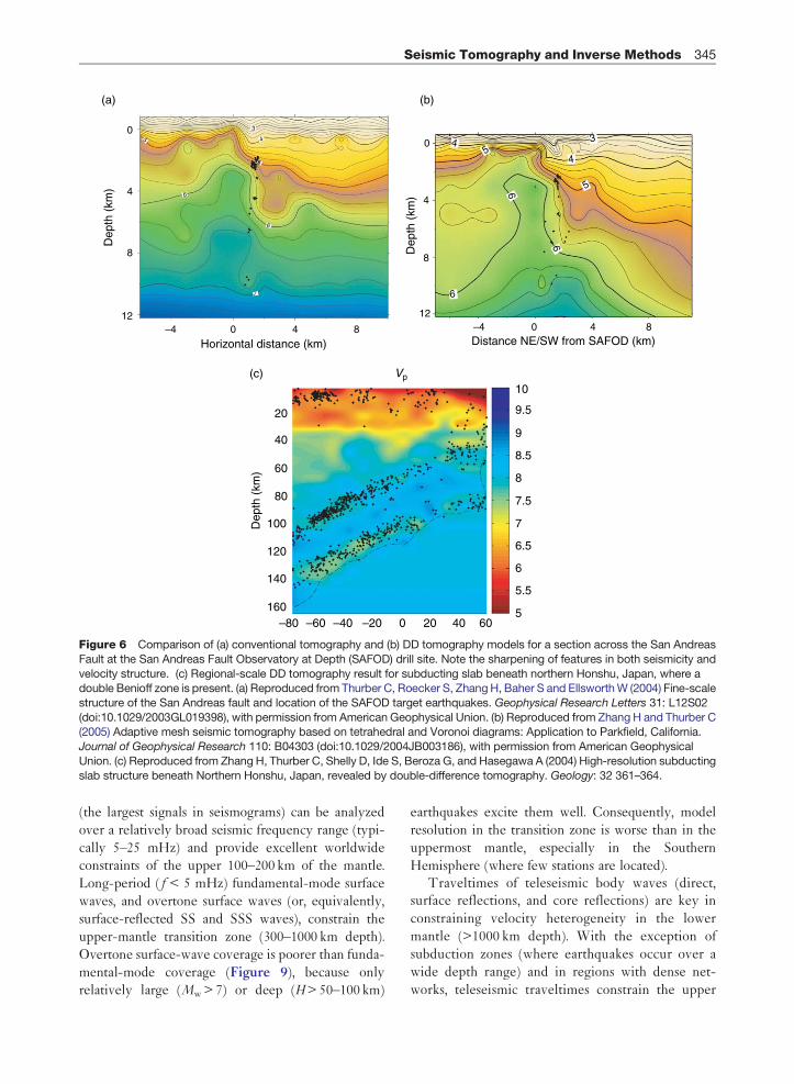
0

4 6

6

5

3

7

4

5

8

12

Horizontal distance (km)

Dep

th (

km)

Dep

th (

km)

–412

8

4

05

4

6

4

3

56

6

0 4 8Distance NE/SW from SAFOD (km)

–4 0 4 8

20

(c)

(a) (b)

Vp

10

9.5

9

8.5

8

7.5

7

6.5

6

5.5

5

40

60

80

100Dep

th (

km)

120

140

160–80 –60 –40 –20 0 20 40 60

Figure 6 Comparison of (a) conventional tomography and (b) DD tomography models for a section across the San Andreas

Fault at the San Andreas Fault Observatory at Depth (SAFOD) drill site. Note the sharpening of features in both seismicity and

velocity structure. (c) Regional-scale DD tomography result for subducting slab beneath northern Honshu, Japan, where adouble Benioff zone is present. (a) Reproduced from Thurber C, Roecker S, Zhang H, Baher S and Ellsworth W (2004) Fine-scale

structure of the San Andreas fault and location of the SAFOD target earthquakes. Geophysical Research Letters 31: L12S02

(doi:10.1029/2003GL019398), with permission from American Geophysical Union. (b) Reproduced from Zhang H and Thurber C(2005) Adaptive mesh seismic tomography based on tetrahedral and Voronoi diagrams: Application to Parkfield, California.

Journal of Geophysical Research 110: B04303 (doi:10.1029/2004JB003186), with permission from American Geophysical

Union. (c) Reproduced from Zhang H, Thurber C, Shelly D, Ide S, Beroza G, and Hasegawa A (2004) High-resolution subducting

slab structure beneath Northern Honshu, Japan, revealed by double-difference tomography. Geology: 32 361–364.


(the largest signals in seismograms) can be analyzed

over a relatively broad seismic frequency range (typi-

cally 5–25 mHz) and provide excellent worldwideconstraints of the upper 100–200 km of the mantle.

Long-period ( f < 5 mHz) fundamental-mode surface

waves, and overtone surface waves (or, equivalently,

surface-reflected SS and SSS waves), constrain the

upper-mantle transition zone (300–1000 km depth).

Overtone surface-wave coverage is poorer than funda-

mental-mode coverage (Figure 9), because onlyrelatively large (Mw > 7) or deep (H > 50–100 km)

earthquakes excite them well. Consequently, model

resolution in the transition zone is worse than in the

uppermost mantle, especially in the Southern

Hemisphere (where few stations are located).Traveltimes of teleseismic body waves (direct,

surface reflections, and core reflections) are key in

constraining velocity heterogeneity in the lower

mantle (>1000 km depth). With the exception of

subduction zones (where earthquakes occur over a

wide depth range) and in regions with dense net-

works, teleseismic traveltimes constrain the upper

0

2019

1817 16

151413

1211

10

Angular order9

87

65

43

21

0

27002400

21001800

1500

Depth (km)1200

900600

300

1/12 1/6 2/6 3/6rms amplitude

4/6 5/6 1

Figure 7 Spectral amplitude of shear velocity heterogeneity in model S20RTS as a function of depth and angular order l.

Note that the amplitude spectrum is largest at the boundary layers of the mantle (surface, core–mantle boundary, the 660 kmphase transition) and that it is predominantly ‘red’, meaning that the spectral amplitudes decrease significantly beyond order

l¼8 (i.e., shear-velocity variations with wavelengths longer than about �5000 km).


mantle poorly (Figure 10) because body waves pro-pagate steeply through it.

An understanding of surface-wave and body-wavecoverage helps us to gain insight in understanding thefirst-order differences between the S- and P-wavemodels of Figure 8. Surface-wave data are onlyincorporated in S models, and they are the keydata to constrain the lithospheric structure. TheS-velocity models feature relatively strong (�15%)velocity variations in the upper 200 km that correlatewith surface geology (e.g., high velocities in the old-est regions of continents), and plate tectonics (e.g.,mid-ocean ridges, oceanic plate ages). The P modelslack these features as traveltime data provide extre-mely poor upper-mantle resolving power. The broadhigh-velocity structure in the western Pacific transi-tion zone is likely a signature of slab flattening abovethe 660-km phase transition. The P models featureupper-mantle slab structures in much more detail.However, the incomplete transition zone sampling(i.e., ocean basins and Africa), especially in modelP-MIT that is based on direct P wave only, makesit still difficult to place transition zone heterogeneityin a global context. Moreover, the high correlationbetween the maps for depths of 125 km and 600 km in

the P-wave models (note, e.g., the signature of theAfrican cratons throughout the upper mantle) is awell-understood artifact due to the relatively poorvertical resolution in the upper mantle.

The lowermost mantle (D0) is ideally constrained byshear-wave core reflections (i.e., ScS) and core diffrac-tions (Sdiff). P-wave counterparts of these waves (e.g.,PcP, Pdiff) have small amplitudes. ISC catalogs, in parti-cular, lack reliable Pdiff traveltime data as these signalsare especially difficult to detect in short-period seismo-grams. Therefore, velocity heterogeneity in D0 isprobably best resolved in S models. S models includebroad low-velocity anomalies beneath Africa and thePacific that are less conspicuous in P models. Some ofthe differences in S- and P-velocity heterogeneity maybe real (e.g., Masters et al., 2000). We note however, thatmodels which include long-period Pdiff traveltime data,such as model FF-PRI and an updated version ofP-MIT (Karason and van der Hilst, 2001), show theAfrican and Pacific anomalies with more clarity, under-scoring that data coverage is playing a key role in theresolution of velocity heterogeneity.

Heterogeneity in the mid-mantle (1000–2500 kmdepth) is primarily constrained by traveltimes orbody waveforms. Since all models in Figure 8

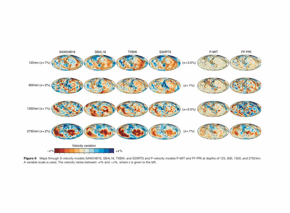
SAW24B16 SB4L18 TXBW S20RTS

(x = 3.5%)

(x = 1%)

(x = 1%)

(x = 0.5%)

125 km (x = 7%)

600 km (x = 2%)

1350 km (x = 1%)

2750 km (x = 2%)

Velocity variation

–x % +x %

P-MIT FF-PRI

Figure 8 Maps through S-velocity models SAW24B16, SB4L18, TXBW, and S20RTS and P-velocity models P-MIT and FF-PRI at depths of 125, 600, 1350, and 2750 km.

A variable scale is used. The velocity varies between –x% and þx%, where x is given to the left.

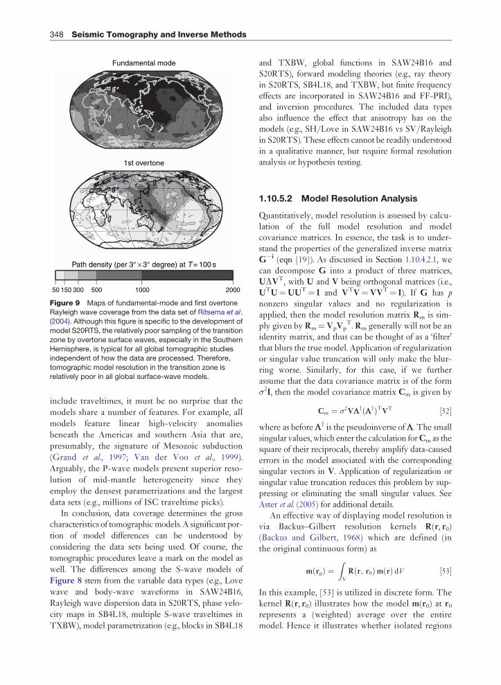
Fundamental mode

1st overtone

Path density (per 3° × 3° degree) at T = 100 s

50 150 300 500 1000 2000

Figure 9 Maps of fundamental-mode and first overtoneRayleigh wave coverage from the data set of Ritsema et al.

(2004). Although this figure is specific to the development of

model S20RTS, the relatively poor sampling of the transition

zone by overtone surface waves, especially in the SouthernHemisphere, is typical for all global tomographic studies

independent of how the data are processed. Therefore,

tomographic model resolution in the transition zone isrelatively poor in all global surface-wave models.


include traveltimes, it must be no surprise that the

models share a number of features. For example, all

models feature linear high-velocity anomalies

beneath the Americas and southern Asia that are,

presumably, the signature of Mesozoic subduction

(Grand et al., 1997; Van der Voo et al., 1999).

Arguably, the P-wave models present superior reso-

lution of mid-mantle heterogeneity since they

employ the densest parametrizations and the largest

data sets (e.g., millions of ISC traveltime picks).In conclusion, data coverage determines the gross

characteristics of tomographic models. A significant por-

tion of model differences can be understood by

considering the data sets being used. Of course, the

tomographic procedures leave a mark on the model as

well. The differences among the S-wave models of

Figure 8 stem from the variable data types (e.g., Love

wave and body-wave waveforms in SAW24B16,

Rayleigh wave dispersion data in S20RTS, phase velo-

city maps in SB4L18, multiple S-wave traveltimes in

TXBW), model parametrization (e.g., blocks in SB4L18

and TXBW, global functions in SAW24B16 andS20RTS), forward modeling theories (e.g., ray theoryin S20RTS, SB4L18, and TXBW, but finite frequencyeffects are incorporated in SAW24B16 and FF-PRI),and inversion procedures. The included data typesalso influence the effect that anisotropy has on themodels (e.g., SH/Love in SAW24B16 vs SV/Rayleighin S20RTS). These effects cannot be readily understoodin a qualitative manner, but require formal resolutionanalysis or hypothesis testing.

1.10.5.2 Model Resolution Analysis

Quantitatively, model resolution is assessed by calcu-lation of the full model resolution and modelcovariance matrices. In essence, the task is to under-stand the properties of the generalized inverse matrixG�i (eqn [19]). As discussed in Section 1.10.4.2.1, wecan decompose G into a product of three matrices,U�VT, with U and V being orthogonal matrices (i.e.,UTU¼UUT¼ I and VTV¼VVT¼ I). If G has p

nonzero singular values and no regularization isapplied, then the model resolution matrix Rm is sim-ply given by Rm¼VpVp

T. Rm generally will not be anidentity matrix, and thus can be thought of as a ‘filter’that blurs the true model. Application of regularizationor singular value truncation will only make the blur-ring worse. Similarly, for this case, if we furtherassume that the data covariance matrix is of the form2I, then the model covariance matrix Cm is given by

Cm ¼ 2VLyðLyÞTVT ½52�

where as before Ly is the pseudoinverse of L. The smallsingular values, which enter the calculation for Cm as thesquare of their reciprocals, thereby amplify data-causederrors in the model associated with the correspondingsingular vectors in V. Application of regularization orsingular value truncation reduces this problem by sup-pressing or eliminating the small singular values. SeeAster et al. (2005) for additional details.

An effective way of displaying model resolution isvia Backus–Gilbert resolution kernels R(r, r0)(Backus and Gilbert, 1968) which are defined (inthe original continuous form) as

mðr0Þ ¼Z

V

Rðr; r0ÞmðrÞ dV ½53�

In this example, [53] is utilized in discrete form. Thekernel R(r, r0) illustrates how the model m(r0) at r0

represents a (weighted) average over the entiremodel. Hence it illustrates whether isolated regions

170–510 km 850–1190 km

1360–1700 km 1870–2210 km

2380–2720 km

Path density (per 3° × 3° degree)

5025 100 175 250 500

Figure 10 Maps of teleseismic body wave (S, SS, SSS, SKS, SKKS, ScS, ScS2) wave coverage from the data set ofRitsema et al. (2004). Although this figure is specific to the development of model S20RTS, it is typical that teleseismic body

wave coverage is best in the mid-mantle (1000–2000 km depth) and relatively poor in the upper mantle (0–1000 km).

Uppermost mantle sampling is excellent only in subduction zones and regions with dense seismic networks.


of the model of the mantle are independentlyresolved. Figure 11 shows four Backus–Gilbert ker-nels computed for model S20RTS. The relativelybroad lateral extents of these kernels reflect thecoarse degree-20 parametrization of S20RTS, whilethe variable vertical extent is, again, an indication ofthe heterogeneous model resolution (velocity varia-tions with wavelengths shorter than 2000 km at theEarth’s surface are unresolved). Resolution is best inthe uppermost mantle (0–200 km) (Figure 11(a)).Here, S20RTS employs a relatively fine spline

parametrization (Ritsema et al., 2004), and this regionis well sampled by fundamental-mode Rayleighwaves. Vertical resolution is poor in the transitionzone. The Backus–Gilbert kernel computed for adepth of 350 km and the location south of NewZealand (Figure 11(b)) is broad, reflecting the poorvertical resolution in the transition zone, especially inthe Southern Hemisphere. Therefore, the low-velocity structure in this region, which is prominentin S20RTS (as well as SB4L18), has an uncertainvertical extent. The Backus–Gilbert kernel in

(a) (b)

(c) (d)

0 0.5 1.0

2004006008001000

Depth (km

)

Depth (km

)D

epth (km)

Depth (km

)

1200140016001800

150 km 350 km

575 km 1075 km

0 0.5 1.0

20040060080010001200140016001800

0 0.5 1.0

20040060080010001200140016001800

0 0.5 1.0

20040060080010001200140016001800

Figure 11 Backus–Gilbert resolution kernels for locations beneath (a) Western Australia (150 km depth), (b) Southwest

Pacific (350 km depth), (c) Mariana Islands (575 km depth), (d) Southeast Asia (1075 km) for model S20RTS. Map views are

shown on the left. Vertical cross sections through the kernels are shown on the right. The geographic variability of these

kernels reflects the heterogeneous mantle resolution, typical for any tomographic model.


Figure 11(c) has a narrower depth extent, given therelatively high data coverage of the western Pacificby both body waves and overtone Rayleigh waves.Finally, the Backus–Gilbert kernel at 1075 km depth(Figure 11(d)) beneath Southeast Asia is less than200 km wide. Given this relatively narrow extent, wemay conclude that the high-velocity anomaly in thisregion of the mantle is resolved independently fromanomalies shallower in the mantle. Hence, it appearsnot to be an artifact from vertical averaging of high-velocity (slab) structure in the transition zone ofIndonesia.

While formal resolution tests are feasible for mod-erately large inversions (e.g., Ritsema et al., 1999; Ishii

and Tromp, 1999; Kuo and Romanowicz, 2002) whenthe model comprises fewer than 10 000 parameters,

they become ultimately impractical for extremelylarge problems. Boschi (2003) and Soldati and

Boschi (2005) provide some enlightening discussionsof whole-Earth model resolution matrix calculations.Beginning with Nakanishi and Suetsugu (1986), a

number of authors have proposed methods for deriv-ing approximate model resolution and/or covariance

matrices (Zhang and McMechan, 1995; Nolet et al.,1999; Yao et al., 1999). The effectiveness and

efficiency of these methods has been subject tosome debate. Displaying such results is also proble-matic, since both matrices have dimensions equal tothe number of model parameters. One strategy forcompressing the full resolution matrix into a compactform that can be displayed in a manner like that ofthe model itself is resolution spread (Michelini andMcEvilly, 1991), which produces a scalar field quan-tifying the spatial extent of blurring at each point inthe model.

1.10.5.3 Hypothesis Testing

An entirely different strategy for evaluating the qual-ity of a tomographic model involves hypothesis tests.In such tests, it is determined how a hypotheticalstructure of the Earth would be recovered tomogra-phically. There are two ways to approach such tests.One could evaluate the resolution operator Rm,which is defined as [29]:

mout ¼ Rmmin ½54�

Simply convolving Rm with a conceptual inputmodel min renders mout which is the tomographically


resolved structure if min were the true Earth. Thedegree of recovery of min in various parts of mout isused to define the well-resolved parts of the model.Alternatively, one can mimic the effects of [29] byinverting synthetic data generated for min followingthe same procedures that were applied to the real data.Tomographers choose a variety of synthetic struc-tures for min including spikes (isolated anomalies),checkerboards (models with alternating high- andlow-velocity anomalies), and conceptual geologicalstructures.

Figure 12 shows an application to the Icelandicupper mantle, where model S20RTS features a low-velocity anomaly that extends much deeper into theupper mantle than what is typical for the Mid-AtlanticRidge (Figure 12(a)). To assess this extent, we can testhow relative narrow structures (cylinders) with variabledepth extents are projected tomographically. The 200-km-wide cylinders of min are at least 5 times wider inmout (Figure 12(b)). This is entirely due to the para-metrization of model S20RTS (spherical harmonics upto order and degree 20) that cannot accommodatevelocity variations with a half-wavelength smallerthan 1000 km. Furthermore, we can observe verticalstretching of the cylinders due to the finite depth reso-lution. For example, the cylinder that extends from thesurface to a depth of 400 km is projected into mout as ananomaly that reaches the 670 km discontinuity. Therelatively broad averaging lengths deeper in the transi-tion zone are also evident in Figure 12. The peakanomaly of the 100-km-thick cylinder that, in min,was placed immediately below the 660-km discontinu-ity is reduced by about a factor of 6 in mout. While it isimpossible to conclude which true Earth structure isresponsible for the tomographic image of Figure 12(a)(we can only determine mout given min, but not viceversa), it appears that heterogeneity in the mantlebelow the 660 km discontinuity is independentlyresolved from the mantle above it. It is plausible, how-ever, that a low-velocity anomaly in the upper 400–500 km of the mantle is artificially extended to 700 kmdepth. The hypothesis tests of Figure 12 suggest alsothat a lower bound of the Icelandic anomaly is a realfeature.

Another approach is to use geophysically moremeaningful input models. An example is providedin Figure 13. Here an input model (min) is derivedfrom a numerical calculation of mantle convection(McNamara and Zhong, 2005; Ritsema et al., 2007)and mout is obtained by convolving min with Rm.Figure 13 demonstrates how small-scale structuressuch as thermal instabilities from thermochemical

basal structures cannot be resolved at the resolution

of S20RTS (and presumably other global models). In

addition, even large structures in min are artificially

stretched and tilted in mout in regions (e.g., the cen-

tral Pacific lower mantle) with unidirectional mantle

sampling.Hypothesis tests like those in Figures 12 and 13

have serious pitfalls when only a number of cases of

min are tested. One can only infer how min is mapped

tomographically into mout, but not vice-versa

because the components of a model in the null

space of G (the components of V corresponding to

the zero singular values) cannot possibly be resolved.

It is therefore dangerous to generalize the resolution

of a tomographic model from the outcome of only a

few tests. In fact, Leveque et al. (1993) show, perhaps

counterintuitively, that the success of a checkerboard

test to resolve the small-scale checkerboard structure

cannot guarantee that larger-scale structures will be

resolved with the same data set. It is possible for some

small features to be resolvable when some larger-

scale features are not. For instance, they illustrate

how horizontal variations can be well recovered

while the large-scale radial variation is poorly

resolved if most of the rays are subparallel and stee-

ply incident. This is of course an inherent problem of

the teleseismic traveltime inversion, such as the ACH

tomography method (Aki et al., 1977).We also point out that cell-based tomographic

systems have a natural tendency for negative model

covariance between adjacent cells. This is caused by

the fact that, when resolution is imperfect, a positive

perturbation in one cell can be counterbalanced by

negative perturbations in adjacent cells (the exact

pattern of a checkerboard) with little effect on the

data fit. Hence noisy (underdamped or under-

smoothed) tomographic models typically show

oscillatory behavior. Thus, checkerboard tests may

yield overly optimistic estimates of model quality

due to the presence of error in the synthetic data

coupled with the character of the model covariance.‘Model restoration’ tests are another popular

approach. Here, a model with all of the main features

of the model obtained from the real data (sometimes

with the sign of the anomalies reversed; Husen and

Kissling, 2001) is used to generate synthetic observa-

tions, which are then inverted using the same method

and parameters as those used for the real data. When

extended to include comparable assessment of mod-

els lacking some of the key features (Zhang et al.,

2004), this approach can be very effective.

200

400

600

800

1000

1200

1400

Dep

th (

km)

0–200 km 0–300 km 0–400 km 0–500 km

200

400

600

800

1000

1200

1400

Dep

th (

km)

–20 –10 0 10 20

660–860 km

–20 –10 0 10 20

660–960 km

–20 –10 0 10 20

660–1060 km

–20 –10 0 10 20

660–1160 km

Distance (deg) Distance (deg) Distance (deg) Distance (deg)

(b)

200

400

600Dep

th (

km)

40 50

North American Shield Iceland Baltic Shield(a)

800

1000–50 –40 –30 –20 –10 0 10 20 30

Distance (deg)

–3% +3%Shear velocity variation from 1-D

Figure 12 (a) Upper-mantle cross section through model S20RTS, showing a low-velocity anomaly beneath Iceland thatextends to about 800 km depth. (b) ‘Spike tests’ designed to evaluate whether the Icelandic low-velocity anomaly points to a

deeper-than-normal mantle upwelling beneath the Icelandic region of the Mid-Atlantic Ridge, or whether it is a tomography

artifact. The cross sections show mout obtained by convolving hypothetical models min with the resolution operator Rm.The input models min are 200-km-wide cylinders of the mantle beneath Iceland with a uniform velocity perturbation from

the reference model. Their tops are top row at the Earth’s surface or bottom row at the 660 km discontinuity, and their

vertical extent varies from left to right between 100 and 500 km. The numbers indicate to which depth the cylinders in

min extend.


One thorough approach to the quantification ofmodel uncertainty is the use of global optimization

methods, such as Monte Carlo (Mosegaard and

Tarantola, 1995), to explore the range of possible

solutions. Press (1968) took the Monte Carlo

approach for modeling global 1-D Earth structure.

Shapiro and Ritzwoller (2002) applied a Markov-

chain Monte Carlo analysis to a global surface wave

model of crust and upper mantle structure. As one

might expect, the uncertainties that they quantify

substantially exceed standard estimates based on the

model covariance matrix.Given the difficulties of fully evaluating model

resolution and covariance matrices, tomographers

often resort to the kind of simplified hypothesis tests

described above to estimate the significance of

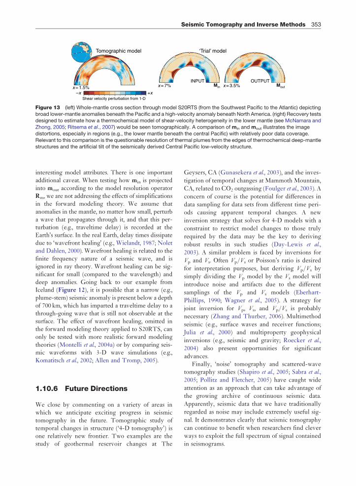
Tomographic model

x = 1.5% x = 7% x = 3.5%INPUT OUTPUT

Min Mout

–x +xShear velocity perturbation from 1-D

‘Trial’ model

Figure 13 (left) Whole-mantle cross section through model S20RTS (from the Southwest Pacific to the Atlantic) depicting

broad lower-mantle anomalies beneath the Pacific and a high-velocity anomaly beneath North America. (right) Recovery testsdesigned to estimate how a thermochemical model of shear-velocity heterogeneity in the lower mantle (see McNamara and

Zhong, 2005; Ritsema et al., 2007) would be seen tomographically. A comparison of min and mout illustrates the image

distortions, especially in regions (e.g., the lower mantle beneath the central Pacific) with relatively poor data coverage.

Relevant to this comparison is the questionable resolution of thermal plumes from the edges of thermochemical deep-mantlestructures and the artificial tilt of the seismically derived Central Pacific low-velocity structure.


interesting model attributes. There is one importantadditional caveat. When testing how min is projectedinto mout according to the model resolution operatorRm, we are not addressing the effects of simplificationsin the forward modeling theory. We assume thatanomalies in the mantle, no matter how small, perturba wave that propagates through it, and that this per-turbation (e.g., traveltime delay) is recorded at theEarth’s surface. In the real Earth, delay times dissipatedue to ‘wavefront healing’ (e.g., Wielandt, 1987; Noletand Dahlen, 2000). Wavefront healing is related to thefinite frequency nature of a seismic wave, and isignored in ray theory. Wavefront healing can be sig-nificant for small (compared to the wavelength) anddeep anomalies. Going back to our example fromIceland (Figure 12), it is possible that a narrow (e.g.,plume-stem) seismic anomaly is present below a depthof 700 km, which has imparted a traveltime delay to athrough-going wave that is still not observable at thesurface. The effect of wavefront healing, omitted inthe forward modeling theory applied to S20RTS, canonly be tested with more realistic forward modelingtheories (Montelli et al., 2004a) or by comparing seis-mic waveforms with 3-D wave simulations (e.g.,Komatitsch et al., 2002; Allen and Tromp, 2005).

1.10.6 Future Directions

We close by commenting on a variety of areas inwhich we anticipate exciting progress in seismictomography in the future. Tomographic study oftemporal changes in structure (‘4-D tomography’) isone relatively new frontier. Two examples are thestudy of geothermal reservoir changes at The

Geysers, CA (Gunasekera et al., 2003), and the inves-

tigation of temporal changes at Mammoth Mountain,

CA, related to CO2 outgassing (Foulger et al., 2003). A

concern of course is the potential for differences in

data sampling for data sets from different time peri-

ods causing apparent temporal changes. A new

inversion strategy that solves for 4-D models with a

constraint to restrict model changes to those truly

required by the data may be the key to deriving

robust results in such studies (Day-Lewis et al.,

2003). A similar problem is faced by inversions for

Vp and Vs. Often Vp/Vs or Poisson’s ratio is desired

for interpretation purposes, but deriving Vp/Vs by

simply dividing the Vp model by the Vs model will

introduce noise and artifacts due to the different

samplings of the Vp and Vs models (Eberhart-

Phillips, 1990; Wagner et al., 2005). A strategy for

joint inversion for Vp, Vs, and Vp/Vs is probably

necessary (Zhang and Thurber, 2006). Multimethod

seismic (e.g., surface waves and receiver functions;

Julia et al., 2000) and multiproperty geophysical

inversions (e.g., seismic and gravity; Roecker et al.,

2004) also present opportunities for significant

advances.Finally, ‘noise’ tomography and scattered-wave

tomography studies (Shapiro et al., 2005; Sabra et al.,

2005; Pollitz and Fletcher, 2005) have caught wide

attention as an approach that can take advantage of

the growing archive of continuous seismic data.

Apparently, seismic data that we have traditionally

regarded as noise may include extremely useful sig-

nal. It demonstrates clearly that seismic tomography

can continue to benefit when researchers find clever

ways to exploit the full spectrum of signal contained

in seismograms.


Acknowledgments

This material is based upon work supported byNational Science Foundation grants EAR-0106666and EAR-0609763 ( JR) and EAR-0346105, EAR-0409291, and EAR-0454511 (CT).

References

Abers GA and Roecker SW (1991) Deep structure of anarc-continent collision: Earthquake relocation and inversionfor upper mantle P and S wave velocities beneath PapuaNew Guinea. Journal of Geophysical Research96: 6370–6401.

Ajo-Franklin JB and Minsley B (2005) Application of minimumsupport constraints to seismic traveltime tomography. EOSTransactions of the America Geophysical Union 86: H13C-1344.

Aki K and Lee WHK (1976) Determination of three-dimensionalvelocity anomalies under a seismic array using first P-arrivaltimes from local earthquakes, 1, a homogeneous initialmodel. Journal of Geophysical Research 81: 4381–4399.

Aki K, Christofferson A, and Husebye ES (1977) Determinationof the three-dimensional seismic structure of the lithosphere.Journal of Geophysical Research 82: 277–296.

Aki K and Richards P (1980) Quantitaive Seismology, Theoryand Methods, 932 pp. San Francisco, CA: W H Freeman.

Allen RM and Tromp J (2005) Resolution of regional seismicmodels: Squeezing the Iceland anomaly. GeophysicalJournal International 161: 373–386.

Anderson DL and Dziewonski AM (1984) Seismic tomography.Scientific American 251: 60–68.

Antolik M, Ekstrom G, Dziewonski AM, Boschi L, Gu YJ, andPan J-F (2000) A new global joint P and S velocity model ofthe mantle parameterized in cubic B-splines.In: Rosenblatt M (ed.) Proceedings of the 22nd Annual DOD/DOE Seismic Research Symposium. New Orleans, LA.Seattle, WC: Kluwer.

Ashiya K, Asano S, Yoshii T, Ishida M, and Nishiki T (1987)Simultaneous determination of the three-dimensional crustalstructure and hypocenters beneath the Kanto–Tokai District,Japan. Tectonophysics 140: 13–27.

Aster RC, Borchers B, and Thurber CH (2005) ParameterEstimation and Inverse Problems, 296 pp. London: Elsevier/Academic Press.

Backus GE and Gilbert JF (1967) Numerical applications of aformalism for geophysical inverse problems. GeophysicalJournal of the Royal Astronomical Society 13: 247–276.

Backus G and Gilbert F (1968) The resolving power of grossEarth data. Geophysical Journal of the Royal AstronomicalSociety 16: 169–205.

Backus G and Gilbert F (1970) Uniqueness in the inversion ofinaccurate gross Earth data. Philosophical Transactions ofthe Royal Society of London A 266: 187–269.

Barber CB, Dobkin DP, and Huhdanpaa HT (1996) TheQuickhull algorithm for convex hulls. ACM Transactions onMathematical Software 22: 469–483.

Battaglia J, Thurber C, Got J-L, Rowe C, and White R (2004)Precise relocation of earthquakes following the June 15,1991 explosion of Mount Pinatubo (Philippines). Journal ofGeophysical Research 109: B07302 (doi:10.1029/2003JB002959).

Benz HM, Chouet BA, Dawson PB, Lahr JC, Page RA, andHole JA (1996) Three-dimensional P and S wave velocity

structure of Redoubt Volcano, Alaska. Journal ofGeophysical Research 101: 8111–8128.

Bhattacharyya J, Masters G, and Shearer P (1996) Global lateralvariations of shear wave attenuation in the upper mantle.Journal of Geophysical Research 101: 22273–22289.

Bijwaard H and Spakman W (1999) Fast kinematic ray tracing offirst- and later-arriving global seismic phases. GeophysicalJournal International 139: 359–369.

Bijwaard H and Spakman W (2000) Non-linear global P-wavetomography by iterated linearized inversion. GeophysicalJournal International 141: 71–82.

Bijwaard H, Spakman W, and Engdahl ER (1998) Closing thegap between regional and global travel time tomography.Journal of Geophysical Research 103: 30055–30078.

Billien M, Leveque JJ, and Trampert J (2000) Global maps ofRayleigh wave attenuation for periods between 40 and 150seconds. Geophysical Research Letters 27: 3619–3622.

Boschi E, Ekstrom G, and Morelli A (eds.) (1996) SeismicModeling of Earth Structure, 572 pp. Rome, Italy: InstitutoNazionale di Geofisica.

Boschi L (2003) Measures of resolution in global body-wavetomography. Geophysical Research Letters 30: 1978(doi:10.1029/2003GL018222).

Boschi L and Dziewonski AM (1999) High and low-resolutionimages of the earth’s mantle: Implications of differentapproaches to tomographic modeling. Journal ofGeophysical Research 104: 25567–25594.

Boschi L and Ekstrom G (2002) New images of the Earth’s uppermantle from measurements of surface wave phase velocityanomalies. Journal of Geophysical Research 107: 2059(doi:10.1029/2000JB000059).

Boschi L, Ekstrom G, and Kustowski B (2004)Multiple resolution surface wave tomography: TheMediterranean region. Geophysical Journal International157: 293–304.

Bube KP and Langan RT (1997) Hybrid �1/ �2 minimization withapplications to tomography. Geophysics 62: 1183–1195.

Butler R, Lay T, Creager K, et al. (2004) The GlobalSeismographic Network surpasses its design goal. EOSTransactions of the American Geophysical Union85: 225–229.

Chen P, Zhao L, and Jordan TH (2007) Full 3D tomography forcrustal structure of the Los Angeles region. Bulletin of theSeismological Society of America (in press).

Chiao LY and Kuo BY (2001) Multiscale seismic tomography.Geophysical Journal International 145: 517–527.

Chou C and Booker JR (1979) A Backus–Gilbert approach tothe inversion of travel time data for three dimensionalvelocity structure. Geophysical Journal of the RoyalAstronomical Society 59: 325–344.

Clayton RW and Hearn TM (1982) A tomographic analysisof lateral velocity variations in Southern California.EOS Transactions of the American Geophysical Union63: 1036.

Committee on the Science of Earthquakes (2003) Living on anActive Earth, 418 pp. Washington, DC: National AcademiesPress.

Constable SC, Parker RL, and Constable CG (1987) Occam’sinversion: A practical algorithm for generating smoothmodels from electromagnetic sounding data. Geophysics52(3): 289–300.

Dahlen FA, Hung SH, and Nolet G (2000) Frechet kernels forfinite-frequency travel times-I. Theory. Geophysical JournalInternational 141: 157–174.

Dahlen FA and Tromp J (1998) Theoretical Global Seismology,1025 pp. Princeton, NJ: Princeton University Press.

Dalton CA and Ekstrom G (2006) Global models of surface-wave attenuation. Journal of Geophysical Research 111:B05317 (doi:10.1029/2005JB003997).


Davis T (2006) SIAM Series on the Fundamentals of Algorithms:Direct Methods for Sparse Linear Systems, 214 pp.New York: PWS Publishing.

Dawson PB, Evans JR, and Iyer HM (1990) Teleseismictomography of the compressional wave velocity structurebeneath the Long Valley region, California. Journal ofGeophysical Research 95: 11021–11050.

Day-Lewis F, Harris JM, and Gorelick S (2003) Time-lapseinversion of crosswell radar data. Geophysics67: 1740–1752.

Deschamps F and Trampert J (2004) Towards a lower mantlereference temperature and composition. Earth and PlanetaryScience Letters 222: 161–175.

DeShon HR, Schwartz SY, Newman AV, et al. (2006)Seismogenic zone structure beneath the Nicoya Peninsula,Costa Rica, from three-dimensional local earthquake P- andS-wave tomography. Geophysical Journal International164: 109–124.

Dorren HJS and Snieder RK (1997) Error propagation in non-linear delay-time tomography. Geophysical JournalInternational 128: 632–638.

Douglas A (1967) Joint epicenter determination. Nature215: 47–48.

Du W, Thurber CH, Reyners M, Eberhart-Phillips D, andZhang H (2004) New constraints on seismicity in theWellington region, New Zealand, from relocated earthquakehypocenters. Geophysical Journal International158: 1088–1102.

Dziewonski AM (1984) Mapping the lower mantle: Determinationof lateral heterogeneity in P velocity up to degree and order 6.Journal of Geophysical Research 89: 5929–5952.

Dziewonski AM and Anderson DL (1981) Preliminary ReferenceEarth Model. Physics of the Earth and Planetary Interiors25: 297–356.

Dziewonski AM, Hager BH, and O’Connell RJ (1977) Large-scale heterogeneities in the lower mantle. Journal ofGeophysical Research 82: 239–255.

Dziewonski AM and Steim JM (1982) Dispersion andattenuation of mantle waves through waveform inversion.Geophysical Journal of the Royal Astronomical Society70: 503–527.

Dziewonski AM and Woodhouse JW (1987) Global images ofthe Earth’s interior. Science 236: 37–48.

Eberhart-Phillips D and Henderson CM (2004) Includinganisotropy in 3-D velocity inversion and application toMarlborough, New Zealand. Geophysical JournalInternational 156: 237–254.

Eberhart-Phillips D (1986) Three-dimensional velocity structurein Northern California Coast Ranges from inversion of localearthquake arrival times. Bulletin of the SeismologicalSociety of America 76: 1025–1052.

Eberhart-Phillips D (1990) Three-dimensional P and S velocitystructure in the Coalinga region, California. Journal ofGeophysical Research 95: 15343–15363.

Ekstrom G, Tromp J, and Larson EW (1997) Measurements andmodels of global surface wave propagation. Journal ofGeophysical Research 102: 8137–8157.

Ellsworth WL (1977) Three-Dimensional Structure of the Crustand Mantle Beneath the Island of Hawaii. PhD Thesis,Massachusetts Institute of Technology, Cambridge.

Engdahl ER, van der Hilst RD, and Buland RP (1998) Globalteleseismic earthquake relocation with improved travel timesand procedures for depth determination. Bulletin of theSeismological Society of America 88: 22–43.

Evans JR and Achauer U (1993) Teleseismic velocitytomography using the ACH method: Theory and applicationto continental-scale studies. In: Iyer HM and Hirahara K(eds.) Seismic Tomography: Theory and Applications,pp. 319–360. London: Chapman and Hall.

Foulger GR, Julian BR, Pitt AM, Hill DP, Malin P, and Shalev E(2003) Three-dimensional crustal structure of Long Valleycaldera, California, and evidence for the migration of CO2

under Mammoth Mountain. Journal of Geophysical Research108(B3): 2147 (doi:10.1029/2000JB000041).

Fukao Y, Widiyantoro S, and Obayashi M (2001) Stagnant slabsin the upper and lower mantle transition region. Reviews ofGeophysics 39: 291–323.

Gee LS and Jordan TJ (1992) Generalized seismological datafunctionals. Geophysical Journal International 111: 363–390.

Giardini D, Li X-D, and Woodhouse JH (1987) Three-dimensional structure of the Earth from splitting in free-oscillation spectra. Nature 325: 405–411.

Gilbert F (1970) Excitation of the normal modes of the Earth byearthquake sources. Geophysical Journal of the RoyalAstronomical Society 22: 223–226.

Gilbert F and Dziewonski AM (1975) An application of normalmode theory to the retrieval of structural parameters andsource mechanism from seismic spectra. PhilosophicalTransactions of the Royal Society of London A 278: 187–269.

Gill PE, Murray W, and Wright MH (1981) Practical Optimization,401 pp. San Diego, CA: Academic Press.

Got JL, Frechet J, and Klein F (1994) Deep fault plane geometryinferred from multiplet relative relocation beneath the southflank of Kilauea. Journal of Geophysical Research99: 15375–15386.

Grand SP (1994) Mantle shear structure beneath the Americasand surrounding oceans. Journal of Geophysical Research99: 11591–11621.

Grand SP, van der Hilst RD, and Widiyantoro S (1997) Globalseismic tomography: A snapshot of convection in the Earth.GSA Today 7: 1–7.

Grand SP (2002) Mantle shear-wave tomography and the fate ofsubducted slabs. Philosophical Transactions of the RoyalSociety of London A 3260: 2475–2491.

Gudmundsson O and Sambridge M (1998) A regionalized uppermantle RUM seismic model. Journal of GeophysicalResearch 103: 7121–7136.

Gunasekera RC, Foulger GR, and Julian BR (2003) Three-dimensional tomographic images of progressive pore-fluiddepletion at the Geysers geothermal area, California. Journalof Geophysical Research 108 (doi:10.1029/2001JB000638).

Hawley BW, Zandt G, and Smith RB (1981) Simultaneousinversion for hypocenters and lateral velocity variations: Aniterative solution with a layered model. Journal ofGeophysical Research 86: 7073–7076.

He X and Tromp J (1996) Normal-mode constraints on thestructure of the mantle and core. Journal of GeophysicalResearch 101: 20053–20082.

Hirahara K (1993) Tomography using both local earthquakesand teleseisms: Velocity and anisotropy – Theory. In: Iyer HMand Hirahara K (eds.) Seismic Tomography: Theory andApplications, pp. 493–518. London: Chapman and Hall.

Hole JA, Brocher TM, Klemperer SL, Parsons T, Benz HM, andFurlong KP (2000) Three-dimensional seismic velocitystructure of the San Francisco Bay area. Journal ofGeophysical Research 105: 13859–13874.

Humphreys E, Clayton RW, and Hager BH (1984) Atomographic image of mantle structure beneath southernCalifornia. Geophysical Research Letters 11: 625–627.

Husen S and Kissling E (2001) Local earthquake tomographybetween rays and waves: Fat ray tomography. Physics of theEarth and Planetary Interiors 123: 127–147.

Inoue H, Fukao Y, Tanabe K, and Ogata Y (1990) Whole mantleP-wave traveltime tomography. Physics of the Earth andPlanetary Interiors 59: 294–328.

Ishii M and Tromp J (1999) Normal-mode and free-air gravityconstraints on lateral variations in velocity and density of theEarth’s mantle. Science 285: 1231–1236.


Ishii M and Tromp J (2001) Even-degree lateral variations in theEarth’s mantle constrained by free oscillations and the free-airgravity anomaly. Geophysical Journal International 145: 77–96.

Iyer HM and Hirahara K (eds.) (1993) Seismic Tomography:Theory and Applications, pp. 319–360. London: Chapmanand Hall.

Jeffrey H and Bullen KE (1958) Seismological Tables, Office ofthe British Association, Burlington House, London.

Jet Propulsion Laboratory (1976) Petroleum explorationassessment: Phase 1 report. JPL Document 5040-32.Pasadena, CA: Jet Propulsion Laboratory.

Julia J, Ammon CJ, Herrmann RB, and Correig AM (2000)Joint inversion of receiver function and surface wavedispersion observations. Geophysical Journal International143: 1–19.

Julian BR, Evans JR, Pritchard MJ, and Foulger GR (2000) Ageometrical error in some computer programs based on theAki–Christofferson–Husebye ACH method of teleseismictomography. Bulletin of the Seismological Society ofAmerica 90: 1554–1558.

Karason H and van der Hilst RD (2001) Tomographic imaging ofthe lowermost mantle with differential times of refracted anddiffracted core phases (PKP, Pdiff). Journal of GeophysicalResearch 106: 6569–6588.

Kennett BLN and Engdahl ER (1991) Traveltimes for globalearthquake location and phase identification. GeophysicalJournal International 105: 429–465.

Kennett BLN, Engdahl ER, and Buland R (1995) Constraints onseismic velocities in the Earth from travel times. GeophysicalJournal International 122: 403–416.

Kennett BLN, Sambridge MS, and Williamson PR (1988)Subspace methods for large inverse problems with multipleparameter classes. Geophysical Journal International94: 237–247.

Kissling E (1988) Geotomography with local earthquake data.Reviews of Geophysics 26: 659–698.

Kissling E, Ellsworth WL, Eberhart-Phillips D, and Kardolfer U(1994) Initial reference models in local earthquaketomography. Journal of Geophysical Reasearch99: 19635–19646.

Koch M (1985) Nonlinear inversion of local seismic travel timesfor the simultaneous determination of the 3-D-velocitystructure and hypocentres-application to the seismic zoneVrancea. Journal of Geophysics 56: 160–173.

Komatitsch D, Ritsema J, and Tromp J (2002) The spectral-element method, Beowulf computing and global seismology.Science 298: 1737–1742.

Kuo C and Romanowicz B (2002) On the resolution of densityanomalies in the Earth’s mantle using spectral fitting ofnormal mode data. Geophysical Journal International150: 162–179.

Laske G (1995) Global observation of off-great circlepropagation of long-period surface waves. GeophysicalJournal International 123: 245–259.

Lebedev S, Nolet G, and van der Hilst RD (1997) Theupper mantle beneath the Philipine sea region fromwaveform inversion. Geophysical Research Letters24: 1851–1854.

Lees JM and Crosson RS (1989) Tomographic inversion forthree-dimensional velocity structure at Mount St. Helensusing earthquake data. Journal of Geophysical Research94: 5716–5728.

Lees JM and Crosson RS (1990) Tomographic imaging of localearthquake delay times for three-dimensional velocityvariation in western Washington. Journal of GeophysicalResearch 95: 4763–4776.

Lees JM and Lindley GT (1994) Three-dimensional attenuationtomography at Loma Prieta: Inverting t� for Q. Journal ofGeophysical Research 99: 6843–6863.

Leveque JJ and Cara M (1985) Inversion of multimode surfacewave data: Evidence for sublithospheric anisotropy.Geophysical Journal International 83: 753–773.

Leveque JJ, Rivera L, and Wittlinger G (1993) On the use of thechecker-board test to assess the resolution of tomographicinversions. Geophysical Journal International 115: 313–318.

Li XD and Romanowicz B (1995) Comparison of globalwaveform inversions with and without considering crossbranch coupling. Geophysical Journal International121: 695–709.

Li XD and Romanowicz B (1996) Global mantle shear velocitymodel developed using nonlinear asymptotic couplingtheory. Journal of Geophysical Research 101: 22245–22273.

Li XD and Tanimoto T (1993) Waveforms of long period body-waves in a slightly aspherical earth. Geophysical JournalInternational 112: 92–112.

Li C, van der Hilst RD, and Toksoz MN (2006) ConstrainingP-wave velocity variations in the upper mantle beneathSoutheast Asia. Physics of the Earth and Planetary Interiors154: 180–195.

Lin CH and Roecker SW (1997) Three-dimensional P-wavevelocity structure of the Bear Valley region of CentralCalifornia. Pure and Applied Geophysics 149: 667–688.

Marquering H and Snieder R (1995) Surface wave mode couplingfor efficient forward modeling and inversion of body wavephases. Geophysical Journal International 120: 186–208.

Masson F and Trampert J (1997) On ACH, or how reliable isregional teleseismic delay time tomography? Physics of theEarth and Planetary Interiors 102: 21–32.

Masters G, Johnson S, Laske G, and Bolton H (1996) A shear-velocity model of the mantle. Philosophical Transactions ofthe Royal Society of London A 354: 1385–1411.

Masters G, Jordan T, Silver P, and Gilbert F (1982) Asphericalearth structure from fundamental spheroidal-mode data.Nature 298: 609–613.

Masters G, Laske G, Bolton H, and Dziewonski A (2000) Therelative behavior of shear velocity, bulk sound speed, andcompressional velocity in the mantle: Implications forchemical and thermal structure. In: Karato S (ed.) AGUMonograph, Vol. 117: Earth’s Deep Interior, pp. 63–87.Washington, DC: AGU.

McNamara AK and Zhong S (2005) Thermochemical piles underAfrica and the Pacific. Nature 437: 1136–1139.

Megnin C and Romanowicz B (2000) The 3-D shear velocitystructure of the mantle from the inversion of body, surfaceand higher mode waveforms. Geophysical JournalInternational 143: 709–728.

Megnin C, Bunge HP, Romanowicz B, and Richards MA (1997)Imaging 3-D spherical convection models: What can seismictomography tell us about mantle dynamics? GeophysicalResearch Letters 24: 1299–1302.

Menke W (1989) Geophysical Data Analysis: Discrete InverseTheory. New York: Academic Press.

Menke W and Schaff D (2004) Absolute earthquake locationswith differential data. Bulletin of the Seismological Society ofAmerica 94: 2254–2264.

Michael AJ (1988) Effects of three-dimensional velocitystructure on the seismicity of the 1984 Morgan Hill,California, aftershock sequence. Bulletin of theSeismological Society of America 78: 1199–1221.

Michelini A (1995) An adaptive-grid formalism for traveltimetomography. Geophysical Journal International 121: 489–510.

Michelini A and McEvilly TV (1991) Seismological studies atParkfield: I. Simultaneous inversion for velocity structure andhypocenters using cubic b-splines parameterization. Bulletinof the Seismological Society of America 81: 524–552.

Montagner JP (1994) Can seismology tell us anything aboutconvection in the mantle? Reviews of Geophysics32: 115–138.


Montagner JP and Tanimoto T (1991) Global upper mantletomography of seismic velocities and anisotropies. Journalof Geophysical Research 96: 20337–20351.

Montelli R, Nolet G, Dahlen FA, Masters G, Engdahl ER, andHung SH (2004a) Finite-frequency tomography reveals avariety of plumes in the mantle. Science 303: 338–343.

Montelli R, Nolet G, Masters G, Dahlen FA, and Hung SH (2004b)Global P and PP traveltime tomography: Rays versus waves.Geophysical Journal International 158: 637–654.

Mooney WD, Laske G, and Masters G (1998) CRUST-5.1: Aglobal crustal model at 5o x 5o. Journal of GeophysicalResearch 103: 727–747.

Mosegaard K and Tarantola A (1995) Monte Carlo sampling ofsolutions to inverse problems. Journal of GeophysicalResearch 100: 12431–12448.

Nakanishi I (1985) Three-dimensional structure beneath theHokkaido–Tohoku region as derived from a tomographicinversion of P-arrival times. Journal of Physics of the Earth33: 241–256.

Nakanishi I and Anderson DL (1982) Worldwide distribution ofgroup velocity of mantle Rayleigh waves as determined byspherical harmonic invesion. Bulletin of the SeismologicalSociety of America 72: 1185–1194.

Nakanishi I and Suetsugu D (1986) Resolution matrix calculatedby a tomographic inversion method. Journal of Physics of theEarth 34: 95–99.

Nakanishi I and Yamaguchi K (1986) A numerical experiment onnonlinear image reconstruction from first-arrival times fortwo-dimensional island arc structure. Journal of Physics ofthe Earth 34: 195–201.

Nataf HC and Ricard Y (1996) 3SMAC: An a priori tomographicmodel of the upper mantle based on geophysical modeling.Physics of the Earth and Planetary Interiors 95: 101–122.

Nataf HC, Nakanishi I, and Anderson DL (1986) Measurement ofmantle wave velocities and inversion for lateral heterogeneityand anisotropy, III, inversion. Journal of GeophysicalResearch 91: 7261–7307.

Nolet G (1985) Solving or resolving inadequate and noisytomographic systems. Journal of Computational Physics61: 463–482.

Nolet G (1987) Seismic Tomography: With Applications inGlobal Seismology and Exploration Geophysics. Dordrecht,The Netherlands: D. Reidel.

Nolet G and Dahlen FA (2000) Wavefront healing and theresolution of seismic delay times. Journal of GeophysicalResearch 105: 19043–19054.

Nolet G, Dahlen FA, and Montelli R (2005) Traveltimes andamplitudes of seismic waves: A re-assessment.In: Levander A and Nolet G (eds.) AGU Monograph Series,Vol. 157: Seismic Earth: Analysis of BroadbandSeismograms, pp. 37–48. Washington, DC: AGU.

Nolet G and Montelli R (2005) Optimal parametrization oftomographic models. Geophysical Journal International161: 365–372.

Nolet G, Montelli R, and Virieux J (1999) Explicit, approximateexpressions for the resolution and a posteriori covariance ofmassive tomographic systems. Geophysical JournalInternational 138: 36–44.

Nolet G and Snieder R (1990) Solving large linear inverseproblems by projection. Geophysical Journal International103: 565–568.

Novotny M (1981) Two methods of solving the linearized two-dimensional inverse seismic kinematic problem. Journal ofGeophysics 50: 7–15.

Paige CC and Saunders MA (1982) LSQR: Sparse linearequations and least squares problems. ACM Transactionson Mathematical Software 8: 195–209.

Pavlis GL and Booker JR (1980) The mixed discrete-continuousinverse problem: Application to the simultaneous

determination of earthquake hypocenters and velocitystructure. Journal of Geophysical Research 85: 4801–4810.

Parker RL (1994) Geophysical Inverse Theory, 386 pp.Princeton, NJ: Princeton University Press.

Phillips WS, Hartse HE, and Steck LK (2001) Precise relativelocation of 25 ton chemical explosions at Balapan using IMSstations. Pure and Applied Geophysics 158: 173–192.

Pollitz FF and Fletcher JP (2005) Waveform tomography ofcrustal structure in the south San Francisco bay region.Journal of Geophysical Research 110: B08308 (doi:10.1029/2004JB003509).

Press F (1968) Earth models obtained by Monte Carlo inversion.Journal of Geophysical Research 73: 5223–5234.

Rawlinson N and Sambridge M (2003) Seismic traveltimetomography of the crust and lithosphere. Advances inGeophysics 46: 81–197.

Reagan RL (1978) A Finite-Difference Study of SubterraneanCavity Detection and Seismic Tomography. 229 pp. PhDThesis, University of Missouri-Rolla.

Reid FJL, Woodhouse JH, and van Heijst HJ (2001) Uppermantle attenuation and velocity structure frommeasurements of differential S phases. Geophysical JournalInternational 145: 615–630.

Resovsky JS and Ritzwoller MH (1999) A degree 8 mantle shearvelocity model from normal mode observation below 3 mHz.Journal of Geophysical Research 104: 993–1014.

Rietbrock A (2001) P-wave attenuation structure in the fault areaof the 1995 Kobe earthquake. Journal of GeophysicalResearch 106: 4141–4154.

Ritsema J, Rivera LA, Komatitsch D, Tromp J, and vanHeijst H-J (2002) Effects of crust and mantle heterogeneityon PP/P and SS/S amplitude ratios. Geophysical ResearchLetters 29: 1430 (doi:10.1029/2001GL013831).

Ritsema J, van Heijst HH, and Woodhouse JH (1999) Complexshear wave velocity structure imaged beneath Africa andIceland. Science 286: 1925–1928.

Ritsema J, van Heijst HJ, and Woodhouse JH (2004) Globaltransition zone tomography. Journal of GeophysicalResearch 109: B02302 (doi:10.1029/2003JB002610).

Ritsema J, McNamara AK, and Bull A (2007) Tomographic filteringof geodynamic models: implications for model interpretationand large-scale mantle structure. Journal of GeophysicalResearch 112: B01303 (doi: 10.1029/2006JB004566).

Ritzwoller MH and Laveley EM (1995) Three-dimensionalseismic models of the Earth’s mantle. Reviews ofGeophysics 33: 1–66.

Ritzwoller MH, Levshin AL, Ratnikova LI, and Egorkin AA (1998)Intermediate period group velocity maps across CentralAsia, Western China, and parts of the Middle East.Geophysical Journal International 134: 315–328.

Rodi WL, Jordan TH, Masso JF, and Savino JM (1981)Determination of the three-dimensional structure of easternWashington from the joint inversion of gravity andearthquake data. Systems Sciences and Software ReportSSS-R-80-4516, La Jolla, CA.

Roecker SW (1982) Velocity structure of the Pamir–Hindu Kushregion; possible evidence of subducted crust. Journal ofGeophysical Research 87: 945–959.

Roecker S, Thurber C, and McPhee D (2004) Joint inversion ofgravity and arrival time data from Parkfield: New constraintson structure and hypocenter locations near the SAFOD drillsite. Geophysical Research Letters 31: L12S04 (doi:10.1029/2003GL019396).

Roecker S, Thurber C, Roberts K, and Powell L (2006) Refiningthe image of the San Andreas Fault near Parkfield, Californiausing a finite difference travel time computation technique.Tectonophysics 424 (doi:10.1016/j.tecto.2006.02.026).

Romanowicz B, Cara M, Fels JF, and Rouland D (1984)Geoscope: A French initiative in long period three


component seismic networks. EOS Transactions of theAmerican Geophysical Union 65: 753–754.

Romanowicz B (1991) Seismic tomography of the Earth’s mantle.Annual Review of Earth and Planetary Science 19: 77–99.

Romanowicz B (2003) Global mantle tomography: Progressstatus in the past 10 years. Annual Review of Earth andPlanetary Science 31: 303–328.

Rowe CA, Aster RC, Phillips WS, Jones RH, Borchers B, andFehler MC (2002) Using automated, high-precision repickingto improve delineation of microseismic structures at theSoultz geothermal reservoir. Pure and Applied Geophysics159: 563–596.

Rubin A, Gillard D, and Got JL (1998) A re-examination ofseismicity associated with the January 1983 dike intrusion atKilauea volcano, Hawaii. Journal of Geophysical Research103: 10003–10015.

Sabra KG, Gerstoft P, Roux P, and Kuperman WA (2005)Surface wave tomography from microseisms in southernCalifornia. Geophysical Research Letters 32: L14311(doi:10.1029/2005GL023155).

Sambridge MS (1990) Non-linear arrival time inversion:Constraining velocity anomalies by seeking smooth modelsin 3-D. Geophysical Journal International 102: 653–677.

Sambridge M and Faletic R (2003) Adaptive whole Earthtomography. Geochemistry, Geophysics, Geosystems,4(3): 1022 (doi:10.1029/2001GC000213).

Sambridge M and Gudmundsson O (1998) Tomographicsystems of equations with irregular cells. Journal ofGeophysical Research 103(B1): 773–781.

Sambridge M and Mosegaard K (2002) Monte Carlo methods ingeophysical inverse problems. Reviews of Geophysics40: 3-1–3-29 (doi:10.1029/2000RG000089).

Sambridge M and Rawlinson N (2005) Seismic tomography withirregular meshes. In: Levander A and Nolet G (eds.) AGUGeophysical Monograph series, Vol. 157: Seismic Earth:Array Analysis of Broadband Seismograms, pp. 49–65.Washington, DC: AGU. (doi:10.1029/156GM04).

Scherbaum F (1990) Combined inversion for the three-dimensionalQ structure and source parameters using microearthquakespectra. Journal of Geophysical Research 95: 12423–12438.

Scales JA (1987) Tomographic inversion via the conjugategradient method. Geophysics 52(2): 179–185.

Scales JA and Snieder R (1997) To Bayes or not to Bayes?Geophysics 62(4): 1045–1046.

Selby ND and Woodhouse JH (2002) The Q structure of theupper mantle: Constraints from Rayleigh wave amplitudes.Journal of Geophysical Research 107: 2097 (doi:10.1029/2001JB000257).

Sengupta MK and Toksoz MN (1976) Three dimensional modelof seismic velocity variation in the Earth’s mantle.Geophysical Research Letters 3(2): 84–86.

Shapiro NM, Campillo M, Stehly L, and Ritzwoller MH (2005)High-resolution surface-wave tomography from ambientseismic noise. Science 307: 1615–1618.

Shapiro NM and Ritzwoller MH (2002) Monte-carlo inversion fora global shear-velocity model of the crust and upper mantle.Geophysical Journal International 151: 88–105.

Silver PG (1996) Seismic anisotropy beneath the continents:Probing the depths of geology. Annual Review of Earth andPlanetary Science 24: 385–432.

Snieder R (1990) A perturbative analysis of non-linear inversion.Geophysical Journal International 101: 545–556.

Snieder R and Sambridge M (1992) Ray perturbation theory fortraveltimes and ray paths in 3-D heterogeneous media.Geophysical Journal International 109: 294–322.

Snieder R and Spencer C (1993) A unified approach to raybending, ray perturbation and paraxial ray theories.Geophysical Journal International 115: 456–470.

Soldati G and Boschi L (2005) The resolution of whole Earthseismic tomographic models. Geophysical JournalInternational 161: 143–153.

Spakman W and Bijwaard H (2001) Optimization of cellparameterization for tomographic inverse problems. Pureand Applied Geophysics 158: 1401–1423.

Spakman W and Nolet G (1988) Imaging algorithms: Accuracyand resolution in delay time tomography. In: Vlaar NJ,Nolet G, Wortel M, and Cloetingh S (eds.) MathematicalGeophysics: A Survey of Recent Developments inSeismology and Geodynamics, pp. 155–188. Dordrecht, TheNetherlands: D Reidel.

Spencer C and Gubbins D (1980) Travel-time inversion forsimultaneous earthquake location and velocity structuredetermination in laterally varying media. Geophysical Journalof the Royal Astronomical Society 63: 95–116.

Steck L, Thurber C, Fehler M, et al. (1998) Crust and uppermantle P-wave velocity structure beneath the Valles Caldera,New Mexico: Results from the JTEX teleseismic experiment.Journal of Geophysical Research 103: 24301–24320.

Su WJ and Dziewonski AM (1991) Predominance of long-wavelength heterogeneity in the mantle. Nature352: 121–126.

Su WJ and Dziewonski AM (1992) On the scale of mantleheterogeneity. Physics of the Earth and Planetary Interiors74: 29–54.

Su WJ, Woodward RL, and Dziewonski AM (1994) Degree 12model of shear velocity heterogeneity in the mantle. Journalof Geophysical Research 99: 4945–4980.

Symons NP and Crosson RS (1997) Seismic velocity structureof the Puget Sound region from 3-D non-linear tomography.Geophysical Research Letters 24(21): 2593–2596.

Tarantola A (2005) Inverse Problem Theory and Methods forModel Parameter Estimation, 342 pp. Philadelphia, PA:Society for Industrial and Applied Mathematics.

Tarantola A and Nercessian A (1984) Three-dimensionalinversion without blocks. Geophysical Journal of the RoyalAstronomical Society 76: 299–306.

Tarantola A and Valette B (1982) Generalized nonlinear inverseproblems solved using the least squares criterion. Reviewsof Geophysics and Space Physics 20: 219–232.

Thomson CJ and Gubbins D (1982) Three-dimensionallithospheric modeling at NORSAR: Linearity of the methodand amplitude variations from the anomalies. GeophysicalJournal International 71: 1–36.

Thurber CH (1983) Earthquake locations and three-dimensionalcrustal structure in the Coyote Lake area, central California.Journal of Geophysical Research 88: 8226–8236.

Thurber CH (1992) Hypocenter–velocity structure coupling inlocal earthquake tomography. Special Issue: LateralHeterogeneity and Earthquake Location. Physics of the Earthand Planetary Interiors 75: 55–62.

Thurber CH (2003) Seismic tomography of the lithosphere withbody-waves. Pure and Applied Geophysics 160: 717–737.

Thurber CH and Aki K (1987) Three-dimensional seismic imaging.Annual Review of Earth and Planetary Sciences 15: 115–139.

Thurber CH and Eberhart-Phillips D (1999) Local earthquaketomography with flexible gridding. Computers andGeosciences 25: 809–818.

Thurber C, Roecker S, Zhang H, Baher S, and Ellsworth W(2004) Fine-scale structure of the San Andreas fault andlocation of the SAFOD target earthquakes. GeophysicalResearch Letters 31: L12S02 (doi:10.1029/2003GL019398).

Thurber C, Trabant C, Haslinger F, and Hartog R (2001) Nuclearexplosion locations at the Balapan, Kazakhstan, nuclear testsite: The effects of high-precision arrival times and three-dimensional structure. Physics of the Earth and PlanetaryInteriors 123: 283–301.

Zhang YS and Tanimoto T (1993) High-resolution global uppermantle structure and plate tectonics. Journal of GeophysicalResearch 98: 9793–9823.

Zhao D (2004) Global tomographic images of mantle plumesand subducting slabs: Insight into deep earth dynamics.Physics of the Earth and Planetary Interiors 146: 3–34.

Zhao D, Hasegawa A, and Horiuchi S (1992) Tomographicimaging of P and S wave velocity structure beneathnortheastern Japan. Journal of Geophysical Research97: 19909–19928.

Zhao L and Jordan TH (1998) Sensitivity of frequency-dependent travel times to laterally heterogeneous,

anisotropic Earth structure. Geophysical JournalInternational 133: 683–704.

Zhao L, Jordan TH, Olsen KB, and Chen P (2005) Frechetkernels for imaging regional earth structure based on three-dimensional reference models. Bulletin of the SeismologicalSociety of America 95: 2066–2080.

Zhou HW (1996) A high resolution P wave model for the top1200 km of the mantle. Journal of Geophysical Research101: 27791–27810.

1.10 Theory and Observations – Seismic Tomography and...

Documents

Transcript of 1.10 Theory and Observations – Seismic Tomography and...