11-year solar cycle in Schumann resonance data as observed...

Sun and Geosphere, 2015; 10: 39-49 ISSN 1819-0839

39

11-year solar cycle in Schumann resonance data as observed in Antarctica

A.P. Nickolaenko1, A.V. Koloskov2, M. Hayakawa3, Yu.M. Yampolski2, O.V. Budanov2, V.E. Korepanov4

1A.Ya. Usikov, Institute for Radiophysics and Electronics, National Academy of Sciences of the Ukraine, 12, Acad. Proskura St., Kharkiv, 64085, Ukraine

2Institute of Radio Astronomy, National Academy of Sciences of the Ukraine, 4 Chervonopraporna St., Kharkiv, 61002, Ukraine

3Hayakawa Institute of Seismo Electromagnetics Co. Ltd., University of Electro-Communications, Incubation Center,

1-5-1 Chofugaoka, Chofu Tokyo 182-8585, Japan 4Lviv Centre of Institute for Space Research, National Academy of Sciences and State

Space Agency of Ukraine, 5-A Naukova St., Lviv, 79060, Ukraine

E mail ([email protected] [email protected] [email protected] [email protected]).

Accepted 16 January 2015

Abstract Studies of Schumann resonance allows obtaining characteristics of the lower ionosphere and the dynamics of global thunderstorms based on the data recorded at a single or a few ground-based observatories. We use the simple model of a point source. The vertical profile of air conductivity is described by the “knee” model. We used continuous Schumann resonance record from the “Akademik Vernadsky” Ukrainian Antarctic station (geographic coordinates: 65.25°S and 64.25°W, L=2.6). A data processing show that the north-south seasonal drift of global thunderstorms was about 20°, and the intensity of global lightning activity changed annually by the factor 1.5–2. Unequal duration of the “electromagnetic” seasons was confirmed (“summer” ~ 120 days, “winter” ~ 60 days; duration of the “spring” is shorter than the “fall”). A possible explanation of inter-annual variations of Schumann resonance parameter follows from changes in the effective height of the lower ionosphere. In this case, we used the spatial thunderstorm distribution following from the annual data of the Optical Transient Detector satellite. We show that recorded inter-annual variations of resonance frequencies and intensities might be attributed to 1–2 km alterations in the knee height of ionosphere. The most realistic mechanism of changes should include both the height variations and the drift of global thunderstorms. Both the processes are governed by solar activity. We also estimated the feasible trend in the equatorial soil surface temperature by 1.6°C corresponding to the inter-annual change of Schumann resonance intensity. © 2015 BBSCS RN SWS. All rights reserved

Keywords: Schumann resonance; point source; source-receiver distance; global thunderstorm activity; ionosphere

Introduction Monitoring and analysis of the world’s lightning is an

important task for many reasons. One of the significant applications for these researches is studying the connection of lightning with climate and weather changes (Williams, 2012). Taking into account the global nature of thunderstorm activity, it is necessary to select appropriate diagnostic tools, which allow estimating the lightning distribution above all our planet. One possible technique for these investigations is survey of the lightning flashes performed from the satellites. Results of several space missions focused on the monitoring of lightning flashes using optical observations (Optical Transient Detector - OTD, Lightning Imaging Sensors - LIS) are presented and discussed in the literature (Christian et al., 2003; Buechler et al., 2014). Common number of flashes on the Earth as well as geographical and seasonal distributions of global thunderstorms were determined from the satellite data and have been analyzed by Christian et al. (2003). It should be noted that satellite

observations of lightning have some limitations: only small part of global thunderstorms can be directly observed at each moment of time, because the field of view of the optical sensor is relatively small (for OTD it is ~0.25% from all surface of the Earth), and efficiency of lightning detection can be limited by the illumination conditions. Therefore, satellite observations give information sufficient for studying long-term peculiarities of global lightning and only in the statistical-probability sense.

Other opportunity to monitor global thunderstorms, which we will use in the current paper, is observation of the electromagnetic background signal within ELF waveband. As recent experimental results demonstrate, the global resonator formed by the shells Earth surface – lower boundary of ionosphere – Schumann resonator (Nickolaenko and Hayakawa, 2002) excited by the thunderstorm activity in ELF band also serves as the indicator of this activity. The fruitfulness of this diagnostic technique was illustrated for example in the work of Williams (1992), where positive correlation between the relative tropical

A.P. Nickolaenko, A.V. Koloskov, et.al, 11-year solar cycle in Schumann resonance data as observed in Antarctica

40

temperatures and the amplitude of the first Schumann resonance for the period of 5.5 years was demonstrated. Potentially Schumann resonance (SR) observation within ELF waveband allow obtaining total response from all the world’s lightning and estimate dynamic of the global thunderstorms, based on the data recorded at single or a few ground-based observatories. It is worth noting that the parameters of SR signals are determined not only by the sources, but by the properties of the lower ionosphere – medium where signal is propagated. On the one hand, this fact permits using SR observations for probing of the lower ionosphere (Füllekrug et al., 2002), but on the other hand, it complicates studying the characteristics of the sources – global thunderstorm activity.

Diagnostic of the world lighting can be performed by comparing observed power spectra of magnetic and electric fields with modeled ones. A variety of numerical and analytical algorithms (e.g. Nickolaenko and Hayakawa, 2002; Williams et al., 2006) as well as models of the sources are used while calculating the parameters of SR signals. The simplest model for the world’s thunderstorms is equatorial point or distributed source following the Sun during a day at the position corresponding to 17-18 hours local time (Bormotov et al., 1972; Nickolaenko and Rabinowicz, 1995; Nickolaenko et al., 1998; Yatsevich et al., 2005; Pechony, 2007; Pechony et al., 2007). Despite apparent simplicity, one source model is still an important tool for obtaining meaningful geophysical information from the SR monitoring records. It can be effectively used for interpreting of one-point observations and separating the effects produced by the dynamic of the source from the influence of medium on the Schumann resonance signal behavior. More sophisticated models assume three independent sources of thunderstorm activity which correspond to three main global lightning centers (Sátori et al., 2003; Koloskov et al., 2005, Sekiguchi et al., 2006; Bezrodny, 2007; Nickolaenko et al., 2012) or use empirical distributions based of the results of meteorological or space observations (World Meteorological Organization, 1956; Christian et al., 2003; Nickolaenko et al., 2006; Pechony 2007). It should be noted, that realistic distribution of global lightning is quite complicated to be reconstructed using the data from single observation point, and the records of several widely separated observatories are required (Shvets et al., 2010; Williams et al., 2014).

The current paper is devoted to interpreting of the long-term observations of SR background signal performed at the Ukrainian Antarctic Station (UAS) “Akademik Vernadsky” (65.25° S and 64.25° W) (Koloskov et al., 2013). There are several continuous long-term SR registrations performed in the world. For example, the 11-year monitoring of resonance parameters was presented, discussed and interpreted in the paper by Sátori et al. (2005). It included the Antarctic records collected at the Arrival Height observatory with a few substantial gaps although. Therefore, our first objective is presenting the

continuous 10-year SR record obtained in Antarctica (polar location provides minimal effect from artificial and natural interference signals).

Our second goal is estimating the parameters of the global thunderstorm activity from Antarctic record. We apply two “ultimate” models of the source in the model computations: the first one is the point source, and the second implies the average global distribution of thunderstorms obtained by the OTD satellite. We address annual and inter-annual trends in SR data discuss and interpret such variations.

Our third objective is evaluating possible global changes in the height of the lower ionosphere, which might be associated with variations and trends observed in Antarctica.

We use the first SR mode frequencies WESNf ,1 and

intensities WESNI ,1 recorded in the horizontal magnetic

field components since they are proportional to the effective source distance D (e.g., Nickolaenko and Hayakawa, 2002, 2014). Relevant wavelength is equal to the Earth circumference, so that oscillations remain practically insensitive to such “insignificant” details as ionosphere non-uniformities or continents where thunderstorm concentrate.

Experimental records and preliminary data processing

Monitoring observations of SR signals are performed at the Ukrainian Antarctic Station, which will be discussed and interpreted here; it was presented in the paper Koloskov et al. (2013), published in Russian. Because these records are main experimental data set for the current paper, we will describe it in more details. Regular observation of SR signals at UAS was started in March 2002 (Bezrodny et al., 2003). Two horizontal orthogonal components of magnetic fields oriented along geographic meridian (South-North – SN channel) and parallel (West-East – WE channel) where continuously recorded within frequency band 0.1-300 Hz using high-sensitive GPS synchronized induction-coil magnetometers developed by Lviv Center of Institute for Space Research. The experimental data are processed as follows. Daily records from SN and WE channels are separated on 10-minutes intervals. We calculate mean power and cross spectra for each interval with frequency resolution 0.1 Hz. So we have 144 spectra for each day. Then we reject the spectra distorted by interference signals and derive monthly averaged data sets - 144 spectra for each month. These arrays of spectra are used to compute monthly averaged arrays of intensities, peak frequencies (for SN and WE channels separately) and polarization characteristics (polarized intensity, ellipticity, position angle, degree of polarization) for first three modes of SR signals. In the current paper we will analyze only intensities and peak frequencies for the first Schumann

mode. Peak frequencies ( ( )i

SNtf1 and ( )i

WEtf1 ) for

every 10-minutes time interval it , 144...1=i are

calculated as the weighted averaged using equation:


41

( ) ( ) ( )∫∫∆+

∆−

∆+

∆−

⋅=

ff

ff

iWESN

ff

ff

iWESN

iWESN

dftfSdftfSftf0

0

0

0

,, ,,,1

, (1)

where: ( )i

SNtfS ,

and ( )i

WEtfS ,

are power spectra calculated for SN and WE channels correspondently,

0f = 8.0 Hz, f∆

= 1.5 Hz. Intensity corresponds to the values of spectra at peak frequencies:

( ) ( )iWESNWESN

iWESN

tfStI ,,1

,,1 =

. Finally, we calculate daily averaged values of peak frequencies

( )iWESNWESN

tff,

1,

1 = and intensities

( )i

WESNWESNtII

,

1

,

1 =

for each month from March 2002 to February 2012. These data are presented in Figure 1. The upper frame in this figure depicts the long-term variations of the normalized intensity of the first SR mode observed in the horizontal magnetic field I1 = I1WE + I1SN. The thick line shows the running average of changes. Smoothing was performed in the time window of ±3 points width. The middle frame in Fig. 1 presents variations of the first peak frequency observed in two orthogonal magnetic field components. The line with crosses corresponds to the HSN field and the line with dots shows the HWE component. To reduce the rapid oscillations of peak frequencies, we applied the moving average of the data with the same window as for thick intensity curve. Dashed gray lines correspond to the yearly averaged peak frequencies. The lower frame illustrates the concurrent variations in the solar activity. The black lines depict the intensity of solar radiation at the 10.7 cm wavelength (the left ordinate), and the gray lines show the Wolf’s number (the right ordinate). The dashed lines in the middle and lower frames present the annually averaged plots. One may observe that solar activity reached the minimum in 2009 and the SR parameters changes “in-phase” with the 11-year solar cycle.

Figure 1: Averaged intensities (top panel) and peak frequencies (middle panel) of first Schumann resonance recorded at the Ukrainian Antarctic Station “Akademik Vernadsky” (65.25° S and 64.25° W) from March 2002 to February 2012 with respect to solar activity indexes (bottom panel) - intensity of solar radiation at the 10.7 cm wavelength and the Wolf’s number

Description of the models For interpreting the results of observations

performed in Antarctica at UAS, we use two models for the world’s thunderstorms: point source model and distribution based on the OTD satellite data. On the first stage, we calculate integral power spectra of electric and magnetic field produced in observation point (UAS) by the above-mentioned models of lightning sources. Then we vary the parameters of the sources and the characteristics of the medium (lower ionosphere) to estimate changes of these parameters within annual and inter-annual time scales by comparing computational results with the experimental data. We assume that the Earth-ionosphere cavity is uniform along the angular coordinates, and the ionosphere is isotropic. The height conductivity profile of the lower ionosphere corresponds to the “knee model” developed by Mushtak and Williams (2002) for obtaining peak frequencies and Q-factors consistent with observations. According to this model, the vertical profile of the atmospheric conductivity is bending at a certain height. This altitude is called the knee height denoted as hKNEE. Above the knee, the conductivity grows faster than below the knee. The complex radio propagation constant ν(f) is calculated from the following expression:

( ) ( ) EM hhkaf2

4121 ++−=ν (2)

Here, a is the radius of the Earth, k = ω/c is the wave

number of the free space, ω is the circular frequency; hE and hM are the electric and magnetic characteristic heights. In the standard knee model of Mushtak and Williams (2002) the complex heights are found from:

( ) ( )

( ) ( )[ ]( ) ( )[ ]ffi

ff

ffhfh

KNEEbaa

KNEEba

KNEEaE KNEE

arctg2

1ln2

1

ln

2

ζζπζ

ζζ

ζ

−−+

++−+

++=

(3)

( ) ( ) ( ) 2ln ** πζζ fiffhfh mmmmM −−= (4)

In Eq.(3) hKNEE = 55 km is the knee height and fKNEE =

10 Hz is knee reference frequency. The height scale of the conductivity profile is ζa = 2.9 km above the knee, and it is ζb = 8.3 km below the knee altitude. Equation (4) implies the following parameters fm

* = 8 Hz and hm

* = 96.5 km. The height scale of the profile near the magnetic height varies with frequency: ζm = ζm

*+ bm (1/f - 1/fm

*) where bm = 20 km and ζm* = 4 km. At the

lower, electric height hE, the conduction current is equal to the displacement current of given frequency f (Greifinger and Greifinger, 1978). This means that the equality condition is held there:

σ(hKNEE) = σKNEE = 2π fKNEE ε0 = 20πε0, (5)

where ε0 = 8.859 10−12 F/m is the permittivity of vacuum. The upper, magnetic height hM accounts for the diffusion of electromagnetic fields into the ionosphere.


42

The magnetic height is found from Greifinger and Greifinger (1978). The following relation is valid here:

σm(hm) = 1 /[4µ02π fm* (ζm)

2] (6)

where µ0 = 4π⋅10−7 Hn/m is the permeability of vacuum; ζm is the scale height of exponential profile in the vicinity of hM (Greifinger and Greifinger, 1978; Mushtak and Williams, 2002; Nickolaenko and Hayakawa, 2002, 2014). Formula (6) physically means that the profile scale height is equal to the electromagnetic wavelength in the medium.

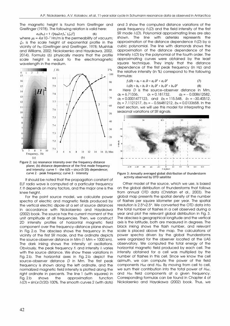
Figure 2: (a) resonance intensity over the frequency–distance plane; (b) distance dependence of the first mode frequency and intensity: curve 1 – the I(D) = sin(π D/20) dependence; curve 2 – peak frequency; curve 3 – intensity

It should be noted that the propagation constant of ELF radio wave is computed at a particular frequency f. It depends on many factors, and the major one is the knee height.

For the point source model, we calculate power spectra of electric and magnetic fields produced by the vertical electric dipole at a set of source distances in accordance with Nickolaenko and Hayakawa (2002) book. The source has the current moment of the unit amplitude at all frequencies. Then, we construct 2D intensity profiles of horizontal magnetic field component over the frequency–distance plane shown in Fig. 2.a. The abscissa shows the frequency in the vicinity of the first SR mode, and the ordinate depicts the source-observer distance in Mm (1 Mm = 1000 km). The dark inking shows the intensity of oscillations. Obviously, the peak frequency f1 and intensity I1 varies with the source distance. We show these variations in Fig. 2.b. The horizontal axes in Fig. 2.b depict the source–observer distance D in Mm. The first peak frequency is shown along the left ordinate, and the normalized magnetic field intensity is plotted along the right ordinate in percents. The line 1 (with squares) in Fig. 2.b shows the approximation function I1(D) = sin(π D/20)⋅100%. The smooth curves 2 (with dots)

and 3 show the computed distance variations of the peak frequency f1(D) and the field intensity of the first SR mode I1(D). Polynomial approximating lines are also shown. The line with asterisks represents the approximation of the distance dependence f1(D) by a cubic polynomial. The line with diamonds shows the approximation of the distance dependence of the intensity I1(D) by the polynomial of the fourth order. The approximating curves were obtained by the least square technique. They imply that the distance dependence of the first peak frequency (in Hz) and the relative intensity (in %) correspond to the following formulas:

f1(D) = a0 + a1⋅D + a2⋅D2 + a3⋅D

3 (7)

I1(D) = b0 + b1⋅D + b2⋅D2 + b3⋅D

3 + b4⋅D4 (8)

Here D is the source–observer distance in Mm, a0 = 6.71336, a1 = 0.181732, a2 = − 0.008612582, a3 = 0.0001477123, and b0 = 115.548, b1 = −30.40512, b2 = 7.1121217, b3 = − 0.56481212, b4 = 0.0133658. In the next section, we will use this model for interpreting the seasonal variations of SR signals.

Figure 3: Annually averaged global distribution of thunderstorm activity observed by OTD satellite

Other model of the source, which we use, is based on the global distribution of thunderstorms that follows from annual OTD data (Christian et al., 2003). The global map presents the spatial density of the number of flashes per square kilometer per year. The spatial resolution is 2.5°×2.5°. We converted the OTD data into the total number of flashes in a cell observed during a year and plot the relevant global distribution in Fig. 3. The abscissa is geographical longitude and the vertical axis is the latitude, both are measured in degrees. The black inking shows the flash number, and relevant scale is placed above the map. The calculations of power spectra driven by the global thunderstorms were organized for the observer located at the UAS observatory. We computed the total energy of the horizontal magnetic field produced by each cell. The intensity obtained for a cell was multiplied by the number of flashes in this cell. Since we know the cell azimuth, we can compute the power of the field components HWE and HSN. By moving from cell to cell, we sum their contribution into the total power of HWE, and HSN field components at a given frequency. Corresponding formulas can be found in Chapter 4 of Nickolaenko and Hayakawa (2002) book. Thus, we


43

estimate the spectral density of the field components produced by the world thunderstorms. Afterwards, frequency is changed, the new ν(f) value is calculated, and the procedure is repeated.

We use the model based on the OTD data for interpreting of inter-annual trends in the SR data recorded at UAS. The possible explanation of these variations may imply changes of the lower ionosphere during the 11-year solar cycle. Formally, the ELF propagation constant depends on the ionosphere profile via the ratio of characteristic magnetic hM and electric hE heights (hM/hE). We consider here variations of the hE caused by changes of the knee height from its regular value of 55 km: it ranges from 45 to 65 km with the step δhKNEE = 1 km. All other parameters of conductivity profile remain constant (see Eq 2-6). After computing power spectra, we combine them into the field intensity maps over the frequency–knee height plane. The maps are shown in Fig. 4.a for the magnetic field components of the first mode of SR - HWE, and HSN. One may observe that small changes of the knee height lead to noticeable alterations in the peak frequency and the peak power. Both of them increase with elevation of the knee height.

Figure 4: (a) changes in the SR spectra in the magnetic field components because of modifications of the knee altitude; (b) dependence of the first peak frequency and peak intensity caused by alteration of the knee altitude: curve 1 depicts the f1 of the field component HWE; curve 2 shows the f1 of the HSN field; curves 3 and 4 show correspondingly the intensities of components HSN and HWE

We show in Fig. 4.b the first peak frequencies and intensities of the orthogonal magnetic field components as functions of the knee height. The abscissa shows the knee height hKNEE in kilometers. The left ordinate shows the maximum frequency in the power spectrum in Hz. Line 1 corresponds to the frequency of the component HWE and line 2 depicts the peak frequency of the HSN field. As might be seen, the peak frequencies of two orthogonal fields vary similarly. The departure of the plots arises from the different orientation of the magnetic antenna having the 8-shape angular patterns superimposed on the

global distribution of thunderstorms. As a result, different field components are sensitive to the lightning strokes at different global thunderstorm centers. The right ordinate in Fig. 4.b shows the peak intensity of the spectra measured in arbitrary units. Line 3 shows the intensity I1 of the field component HSN and line 4 depicts intensity of the HWE field. These also vary similarly, however, they are separated by a wider gap. The departures are also conditioned by the angular pattern of magnetic antennas: it arises from different distances to the field sources in Africa, America, and South-East Asia combined with deviations in their activity.

Processing of data presented in Fig. 4.b by the least squares method provided the linear relationships of the form:

f1= c0 + c1⋅hKNEE (9)

I1= g0 + g1⋅hKNEE (10)

Coefficients in Eq.(9) are c0 = 3.35768; c1 = 7.98×10−2 relevant to the HWE field component and c0 = 3.46903; c1 = 7.88×10−2 for the HSN field. The frequency in Eq.(9) is measured in Hz, and the knee height is measured in kilometers.

Coefficients in Eq.(10) are g0 = −4.34928; g1 = 0.171802 relevant to the HWE field component and g0 = -3.9003; g1 = 0.14492 for the HSN field. The intensity in Eq.(10) is measured in arbitrary units, and the knee height is measured in kilometers. Such a presentation is inconvenient in applications, as the experimental data contain the cumulative intensity of the horizontal magnetic field in (pT)2/Hz. If we average the gk

coefficients of Eq.(10) over the field components and express the model spectral density in absolute units, the following values are obtained: g0 = −0.467; g1 = 1.793×10−2. These coefficients provide the intensity in (pT)2/Hz.

Comparison of the results of model computation with experimental data

Let us use the point source model described in the previous section for interpretation of the peak frequencies variations recorded at UAS within annual time scale. By using equation (7), one can readily correlate the first peak frequency values of 7.7; 7.8; 7.9; and 8.0 Hz with the source distances of 8.3; 12.2; 12.8; and 16 Mm respectively. That is exactly what we did in Fig. 5, where we reproduce the Antarctic monthly averaged first peak frequencies f1 for a particular year of 2006. The months of the year 2006 are shown along the abscissa. The ordinate depicts the observed values of the peak frequency in Hz (left axis) and distance in Mm (right axis). Curve 1 corresponds to the HSN field and the curve 2 presents the HWE component. Frequency variations in the point source model arise from the seasonal drift of thunderstorms. Seasonal northward drift is clearly visible during the boreal summer months, as the distance D from the Antarctic observer to the global thunderstorms increases in both the field components. The separation is estimated as 14 Mm from the SN field component (sensitive to African thunderstorms). Annual drift of these sources


44

reaches 2.4 Mm (in excess of 20°), which is in a rather good agreement with the climatology and independent SR measurements (e.g. Sátori, 2003; Sátori et al., 2003; Hayakawa et al., 2005; Nickolaenko et al., 2006). Variations derived from the WE component (American and Asian thunderstorms) are less pronounced: about 1.5 Mm or 130.

Figure 5: Seasonal patterns of the peak frequencies of the first SR recorded in the HSN (curve 1) and HWE (curve 2) field components at the Ukrainian Antarctic Station “Akademik Vernadsky”

It is worth noting that both estimates exceed 10 Mm. Such a result is surprising, since large distances do not always correspond to climatological data. There might be the following causes of disparity: (i) Different way of evaluating the peak frequency. The values might deviate from those obtained by fitting the resonance peak in the observed spectra. (ii) Deviations might arise from an irrelevant ionospheric model that underestimates the peak frequency. Validity of such an assumption seems doubtful, since the knee model was specially developed for the most exact description of the experimental spectra, although recorded in the Northern hemisphere. (iii) Application of the point source model, which cannot account for the spatial distribution of global thunderstorms. On our opinion the effective distance variation is acceptable, while an additional comparison is desirable between observations and the model computations. Records from the North hemisphere could be very helpful is such a comparison.

Behavior of peak frequencies of the horizontal magnetic field indicates the ultimate northern position

of the global thunderstorms during the June-August season. Moreover, quite reasonable estimates are acquired for the thunderstorm annual drift from the resonance data. These are consistent both with the climatological data, optical observations of the lightning flashes from space (Christian et al., 2003), and with the SR observations in the Northern hemisphere (e.g., Sátori, 2003; Sátori et al., 2003,2005,2012; Pechony, 2007; Pechony et al., 2007; Shvets et al., 2010; Hayakawa et al., 2011; Shvets and Hayakawa, 2011; Williams, 2012). We note that qualitative and quantitative agreement is present in spite the simplest point source model was applied in interpretations. The success of such an interpretation is explained by the relevance of the observed peak frequencies to the distance interval where the f1(D) function is close to a linear one. Therefore, the distance obtained corresponds to the centroid of zone covered by lightning strokes. It is worth noting that seasonal drifts of similar extent were also obtained from the three resonance mode data used in the works by Sátori et al. (2003); Sekiguchi et al. (2006); and Nickolaenko et al. (2012). The latter applied the technique separating the local and universal time variations (Sentman and Fraser, 1991). Similar seasonal source drift was reported by (Sátori, 2003; Sátori et al., 2003, 2005, 2012; Shvets et al., 2010; and Shvets and Hayakawa, 2011).

Figure 6: Seasonal changes of the total intensity of the first SR mode: curve 1 shows the observational data; curve 2 presents the expected variation caused by the distance changes; curve 3 is the intensity of global thunderstorms estimated from the SR records

Fig. 6 demonstrates seasonal variations of the intensity of the first SR mode in 2006. Here, the


45

horizontal axis presents months of 2006, and the vertical axis depicts the intensity of the horizontal magnetic field component in arbitrary units. The observed intensity of resonance oscillations (line 1) has the maximum in summer months and the minimum in boreal winter. The model intensity (curve 2) of resonance oscillations was reconstructed from the Eq. (8) by taking into account the source distance. The latter was derived from the observed peak frequencies by using Eq. (7). We summed the expected intensities of two orthogonal magnetic field components and showed it by curve 2 in Fig. 6. It behaves in a paradoxical way decreasing during boreal summer (June-August). Disparity is quite natural since we applied the source of constant intensity. Contradiction is resolved by accounting for the variable intensity of global thunderstorms: the summer activity increases to an extent overcoming the decrease linked to the northward displacement of the sources. Curve 3 depicts the global lightning activity thus obtained.

One can evaluate the duration of “electromagnetic seasons” from the SR record of Fig. 6. “Electromagnetic summer” lasts from June to September, and this is the period when the source–receiver distance reaches its maximum and the global level of electric activity is the highest. The “electromagnetic winter” lasts from February to March. The source distance is the closest, and thunderstorms are of the weakest level. The remaining intervals correspond to the “spring” and “fall”. Captions in the brackets mark the electromagnetic seasons in Fig. 6.

Thunderstorm intensity thus found varies by the factor of 1.5 during the year, which agrees well with the data obtained at other SR observatories (Sátori, 2003; Sátori et al., 2003,2012; Shvets et al., 2010; Hayakawa et al., 2011; Shvets and Hayakawa, 2011; Nickolaenko et al., 2011; Williams, 2012). Duration of “electromagnetic summer” is about 120 days, whereas the “winter” lasts for about 60 days. The spring period is approximately twice shorter than the autumn one. Unequal duration of seasons in the SR data was noted in the works by (Sátori, 2003; Sátori et al., 2003,2012; and Shvets et al., 2010). All these studies were based on the SR observed in the Northern hemisphere and showed somewhat different duration of seasons. Our data correspond to the Southern hemisphere, and this might cause deviations. At any rate, Antarctic data are qualitatively consistent with the optical observations from space by OTD and LIS satellites (Christian et al., 2003). However, observations of the vertical electric field in the middle Europe showed correspond a longer ‘winter’ (utmost southern) and shorter ‘summer’ (extreme northern) thunderstorm positions (Sátori, 2003; Sátori et al., 2003, 2012). In contrast, Antarctic records, including those presented by Sátori et al. (2005), contain a longer ‘summer’ and a shorter ‘winter’ periods. We note this contradiction, but we have no explanation for this observational fact at present.

The SR monitoring at UAS (see Fig. 1) revealed also a systematic variation of the first peak frequency that

occurred in line with the 11-year solar cycle (Koloskov et al., 2013). Inter-annual changes are driven by the solar activity and allow for dual interpretation (Nickolaenko and Hayakawa, 2002, 2014). Usually, the slow variation is attributed to the inter-annual changes in the ionosphere (Sátori et al., 2005). An alternative explanation connects the SR modifications with a systematic northward-southward drift of global thunderstorms. Validity of this interpretation for the Antarctic data might be verified by the inter-annual frequency variation observed in the Northern hemisphere. Obviously, if the observed changes arise from the seasonal drift of sources, the records in two hemispheres must demonstrate the “mirror behavior”. Observational results presented by Sátori et al. (2005) show that seasonal changes of the first peak frequencies in different hemispheres are antiphased. These facts indicate that they are driven by the seasonal drift of the sources. Meanwhile, the long-term inter-annual variations in the Northern hemisphere (Kułak et al., 2003; Sátori et al., 2005; Ondraskova et al., 2009) demonstrate the similar 11-year trend ‘in-phase’ with the solar activity as in the Southern one. Thus, we must associate the long-term variations of the peak frequencies mainly with the global changes in the lower ionosphere. However, systematic inter-annual drift of global thunderstorms may also exist and provide an additional impact to the observed variation of SR intensities and peak frequencies. Accurate processing of SR data simultaneously recorded in both hemispheres for the time interval comparable with 11-year solar cycle is required to separate the effects produced by changes of the ionosphere from those caused by drift of the sources. Such an analysis is beyond the scope of current work and hopefully may be done in the near future if proper SR records will be available.

Let us employ the OTD model to interpret the inter-annual variations of peak frequencies and intensity observed at UAS (Fig. 1). We will use these data to calculate the knee heights based on the dependences presented in Fig. 4 and equations 9-10. The annually averaged peak frequencies of two components of HWE and HSN are shown in the second and third columns of Table 1. These were converted into the knee heights with the help of Eq. (9). The hKNEE values thus obtained are listed in columns four and five in Table 1. The last two columns contain the annually averaged cumulative peak intensity I1 in (pT)2/Hz and the knee altitude found from the intensity by using Eq.(10).

Thus we obtain three “independent” estimates for the knee height. Figure 7 presents these functions. The years of observations from 2002 to 2011 are plotted on abscissa here. The knee height is shown on the ordinate in km. Lines 1 and 2 show the inter-annual variations of the knee height found from the peak frequency of components HWE and HSN


46

Table 1: Annually averaged peak frequencies of the first SR mode and relevant knee heights

<f1> in different field

components, Hz

hKNEE

deduced from <f1> ,

km

<I1>

cumulative,

(pT)2/Hz

hKNEE

found from <I1>,

km

Year HWE HSN HWE HSN

2002 8.016 7.966 57.74 57.76 0.568 57.75

2003 8.015 7.971 57.72 57.82 0.576 57.39

2004 7.999 7.958 57.40 57.66 0.503 54.39

2005 7.984 7.958 57.33 57.66 0.499 53.66

2006 7.969 7.940 57.14 57.43 0.415 49.17

2007 7.958 7.930 57.00 57.31 0.400 47.97

2008 7.943 7.927 56.81 57.26 0.384 47.33

2009 7.931 7.916 56.66 57.13 0.347 45.41

2010 7.951 7.941 56.91 57.44 0.383 47.4

2011 7.967 7.953 57.11 57.60 0.442 50.72

correspondingly. These heights were found by using Eq. (9). Relevant values are listed in the middle columns of Table 1. Line 3 in Fig. 7 presents the knee height deduced from the cumulative intensity of the first SR mode by using Eq.(10).

Figure 7: Inter-annual variations of the deduced knee heights: curve 1 shows the knee height found from the peak frequency in the HWE record; curve 2 corresponds to peak frequency of HSN field, and curve 3 shows the data found from the records of cumulative field intensity

Figure 7 demonstrates substantial interannual departures of the knee heights found from the peak

frequencies and the field intensity. Difference of curves 1 and 2 is rather small: it reaches almost 1 km while the average knee altitude is about 57 km. Most likely, these deviations arise from the inadequate model allocation of lightning sources over the Earth. However, deviations from the average knee height do not exceed 1%, and this is a rather good coincidence.

The intensity records result in serious departures. Inter-annual alterations of hKNEE definitely go beyond the realistic interval. Indeed, if we accept the hKNEE trend of 10 km, the peak frequency will change by ~0.8 Hz, and such huge variations are absent in observations. However, it is worth noting that UAS is situated in the polar area where variation of knee height may be greater than in the middle and low latitudes, because of influence of energetic charged particles moving along magnetic field lines (Williams et al., 2014). Within long term time-scale a quantity called “auroral power”, which is determined by intensity of electrons precipitations, changes “in-phase” with the 11-year solar cycle with a variation of a factor of two (Zheng et al., 2013). This variation of electron impact can significantly change the profile of conductivity in lower ionosphere (Whitten and Poppoff, 1965) within the range of heights important for Schumann resonance. At the same time, these changes are limited by polar areas, they are irrelevant to the ionosphere of middle and low latitudes, and consequently cannot be accounted within the model of uniform ionosphere, which we use. Besides, the particle precipitation occurs during the magnetic storms only. In spite of active Sun, the auroral power is switched on for relatively short periods of time and thus cannot influence the average lower ionosphere parameters on the inter-annual time scales. Further discussion of this hypothesis will drive us beyond the scope of the current paper.

It is necessary to note that, the overestimated variations might be caused by the fixed intensity of global thunderstorms in the model. When obtaining curve 3 of Fig. 7, we accepted that intensity of global


47

thunderstorms is constant. Possible inter-annual reduction in the thunderstorm activity was attributed to the knee height. To obtain adequate data, one must account for the inter-annual variations of global thunderstorms. Such information is inaccessible at present.

Situation with the knee height might be straightened out if we assume a 1 km drop in hKNEE and the rest of the observed intensity reduction attribute to the changes in global thunderstorm activity. After doing elementary calculations, we obtain that for ∆hKNEE = -1 km, the lightning activity must reduce by the factor of 1.6. This estimate based on the OTD model perfectly agrees with observations and with the reduction obtained in the framework of the point source model.

Summarizing, the estimates of knee height obtained from the UAS observations reach the minimum in 2009. The maximum of the knee height is equal to 57.75 km, it corresponds to the year of 2002 (the active Sun). Application of the annually averaged OTD map provides ambiguous inter-annual hKNEE variations when deduced from resonance intensity since the model does not account for possible inter-annual variations in the thunderstorm activity. On our opinion the realistic height change was about 1 km, and the minimum was reached in 2009 (quiet Sun). Concurrent decrease in the global thunderstorm activity might be estimated by the 1.6 factor.

Discussion We should mention here the interpretation of the

11-year SR data by Sátori et al. (2005) who attributed the inter-annual changes to the upper characteristic height hM of the ionosphere. In this model, the magnetic height decreases with an increase in the solar X-ray flux while the ionosphere around the lower, electric characteristic height hE remains unchanged. As a result, the peak frequency of SR fn ∝ (hE/hM)½ increases. However, to cope with the observed increase in the intensity and the Q-factors, authors had to assert that the upper scale height decreases to extend reducing the novel ζM/hM ratio. This procedure makes the model by Sátori et al. (2005) a two-parametric one. We suggest that the observed variations of peak frequencies and the intensity are associated with changes of a single characteristic height hKNEE. Consequently, the electric height hE also varies. Other parameters of the model are fixed, so that our model is more convenient: we derive a single variable parameter form comparison with observations. Explanation of hKNEE variations may be associated with long-term modulations of the lower ionosphere by changes in the velocity of continuous solar wind that depends on the current solar activity. Plasma of the lower ionosphere is maintained predominantly by the so-called galactic ionizing radiation (Watt, 1967; Viggiano and Arnold, 1995). When activity increases, the average velocity of the solar wind also increases, and it “blows out” the galactic background radiation from the Solar system.

This is the so-called Forbush effect. Thus, the active Sun increases the plasma density in the middle and upper ionosphere, however, a faster solar wind exterminates the lower C-layer of the ionosphere within the range of heights important for Schumann resonance, and all SR parameters increase.

It is interesting to remind that the long-term Antarctic measurements in the VLF band revealed similar alterations in the amplitude of VLF radio transmissions and in the intensity of natural VLF radio noise (Watt, 1967; Bezrodny et al., 1984; Watkins et al., 1998; Thomson and Clilverd, 2000). Similarly to our SR records, the 3 – 4 dB increase was reported in the intensity of both natural noise and the long-distance radio transmissions associated with an increase of the solar activity. It is important to remind that the modern aeronomy data show that the plasma density is modified at heights close to hE. The Monte Carlo computations indicated that the increase in the X- and gamma-rays modifies the ionosphere below the 65–70 km altitudes, see e.g. Inan et al. (2007). Therefore, active Sun provides minor impact around the 100 km altitudes, i.e., the upper characteristic height.

We must also note that transient component of the solar activity (flares, magnetic storms, the corpuscular events) occurs on the short time scales. It is able to temporarily reduce the lower ionosphere edge and to decrease the observed SR parameters: peak frequencies, amplitudes, and the quality factors. Simultaneously, the active sun provides a stronger average solar wind, and the lower ionosphere becomes slightly elevated, the effect is observed as concurrent general increase of the SR parameters and of the average intensity of VLF radio signals.

The inter-annual trend observed in Antarctica of the intensity of the first SR mode is exceptionally similar to changes in the solar activity. Variable solar irradiance might cause alternations in the surface temperature of our planet, primarily, the soil temperature at continents where thunderstorms concentrate. A relationship between changes in the land temperature and the cumulative intensity of SR was analyzed by Sekiguchi et al. (2004, 2006). A high correlation was found between seasonal changes in the resonance intensity (the observatory was located in Japan) and the land temperature in the mid-latitudes. In contrast, the inter-annual trend of resonance power behaved similarly to alterations in the land temperature of tropics (±20° zone around the equator). The relationship was close to linear when the resonance intensity was expressed in dB, and the relevant cross-correlation coefficient was found to be 0.68 for the data series of the 43 months duration.


48

Figure 8: Inter-annual variations: curve 1 shows the temperature anomaly of equatorial soil; curve 2 demonstrates cumulative SR intensity; straight line 3 shows the approximating dependence found by the linear regression

We exploit this result for estimating feasible inter-annual temperature changes. We assume that connection established by Sekiguchi et al. (2004, 2006) persists between the tropical land temperature and the intensity of the SR oscillations regardless the observatory. Relevant data are shown in Fig. 8. Curve 1 corresponds to the temperature anomaly ∆T°C of the soil in the tropical belt. Curve 2 shows the concurrent inter-annual variation of the cumulative SR intensity ∆I in dB. The linear regression between the electromagnetic intensity and the tropical temperature (line 3) provides the following relation:

∆T [0C] = 0.0177 + 0.4845⋅∆I [dB] (11)

The long-term Antarctic measurements of natural VLF radio noise around the 10 kHz frequency allowed Watkins et al. (1998) to suggest a comparable link: a 10% increase in the intensity of radio noise (~0.5 dB) might be associated with a 1°C growth of the global temperature during the period of active Sun. Equation (11) suggests that the alteration in the SR intensity of 1 dB is linked to ~0.5°C alteration of the tropical land temperature.

The UAS SR intensity at the first resonance mode decreased by ~3.2 dB during the 2003-2009 time interval of reducing solar activity (see Fig. 1). In accordance with Eq.(11), the decrease of 1.6°C must occur in the tropical land temperature. Such a trend is quite detectable. We remark that alteration is related

to the soil temperature, while ~80% of tropics are covered by the ocean. The globally averaged estimate of decrease is thus reduced to ~0.3°C, which is still detectable. This trend has no link to the global warming or cooling. This is a regular change in the soil temperature of the tropics related to the 11-year cycle of the solar activity, which was not yet mentioned in literature.

In future, it is desirable to compare the long-term records of SR of the Northern and Southern hemispheres with the tropical temperature. We hope that continuous Antarctic data presented here raise an interest among the SR community and relevant publications will appear very soon

Conclusion The results presented allow for the following

conclusions. 1) The model of a point source confirmed its

efficiency. Reasonable estimates were obtained for seasonal range of the effective source distance by using the UAS records of the first SR mode. The north-south seasonal drift of global thunderstorms was estimated by ~20°.

2) Application of the same model to the records of resonance intensity allowed estimating the annual changes in the global lightning activity by the factor 1.5–2. This estimate agrees with other measurements.

3) Unequal duration of “electromagnetic seasons” was confirmed, which reflect the north–south migration of global thunderstorms. The summer (the extreme northern position) is observed in June–September, and the winter position corresponds to February–March period.

4) Experimental data allow for an alternative interpretation based on changes in the effective height of the global ionosphere. The result is a ~1 km reduction of the ionosphere knee height during 2002–2009 interval when we use the peak frequency records. It exceeds 10 km when derived from the field intensity. The ionosphere lower interface goes down when the solar activity decreases. Such changes are similar to the Forbush effect: a stronger solar wind from active Sun blows out the galactic cosmic rays ionizing the mesosphere and lower ionosphere. The realistic interpretation may combine the latitudinal drift of thunderstorms with variations in the effective height of the lower ionosphere. Both the effects are driven by the Sun.

5) We applied the link derived for the inter-annual trend of cumulative SR intensity and the tropical land temperature. This provided a possible decrease in the tropical land temperature by 1.6 °C toward the minimum of solar activity. Such changes are detectable, and we hope that the statement will be checked.


49

Acknowledgements Authors thank the National Antarctic Science

center of Ukraine for the support of monitoring observations of ELF signals at the Ukrainian Antarctic Station “Akademik Vernadsky”. This work was partially supported by NASU projects “Yatagan-2” (0111U000063) and “Spitsbergen -13, 14” (0113U002656, 0114U002820).

References

Bezrodny V.G.: 2007, J. Atmos. Solar-Terr. Phys. 69(9), 995. doi: 10.1016/j.jastp.2007.03.007.

Bezrodny V.G., Bliokh, P.V., Shubova, R.S., Yampolsky, Yu.M.: 1984, Fluctuations of VLF waves in the Earth – ionosphere cavity, Nauka, Moscow, p. 144.

Bezrodny V.G., Budanov O.V., Koloskov A.V., Yampolski Y.M.: 2003, Kosmicheskaja nauka i tehnologija. 9(5/6), 391.

Bormotov V.N., Lazebny, B.V., Nickolaenko, A.P., Shulga, V.F.: 1972, Geomagnetism and Aeronomia. 12(1), 135.

Buechler D.E., Koshak W.J., Christian H.J., Goodman S.J.: 2014, Atmos. Res. 135–136, 397.

Christian H.J., Blakeslee R.J., Boccippio D.J., Boeck W.L., Buechler D.E, Driscoll K.T., Goodman S.J., Hall J.M., et al.: 2003, J. Geophys. Res. 108(D1), 4005. doi:10.1029/2002JD002347.

Füllekrug M., Fraser-Smith A.C., and Schlegel K.: 2002, Europhys. Lett, 59(4), 626.

Greifinger C., Greifinger P.: 1978, Radio Sci. 13, 831. Hayakawa M., Sekiguchi, M., Nickolaenko, A.P.: 2005, J. Atmos.

Electricity. 25(2), 55. Hayakawa M., Nickolaenko A.P., Shvets, A.V., Hobara, Y.: 2011,

Recent studies of Schumann resonance and ELF transients, in: Wood, M.D. (Ed.) Lightning: Properties, Formation and Types, Nova Sci. Pub., New York, p. 39.

Inan U.S., Lehtinen N.G., Moore R.C., Hurley K., Boggs S., Smith D.M., and Fishman G.J.: 2007, Geophys. Res. Lett. 34. L08103. doi:10.1029/2006GL029145.

Koloskov A.V., Bezrodny V.G., Budanov O.V., Yampolski Y.M.: 2005, Radiofizika i Radioastronomia. 10(1), 11.

Koloskov A.V., Baru, N.A., Budanov O.V., Bezrodny V.G., Gavriluk B.Yu., Paznukhov A.V., Yampolski Yu.M.: 2013, Ukrainian Antarctic Journal. 12, 170.

Kułak A., Kubisz J., Michalec A., Zieba S., Nieckarz Z.: 2003, J. Geophys. Res., 108(A7), 1271. doi:10.1029/2002JA009305.

Mushtak V.C., Williams, E.R.: 2002, J. Atmos. Solar-Terr. Phys. 64, 1989.

Nickolaenko A.P., Rabinowicz, L.M.: 1995, J. Atmos. Solar-Terr. Phys. 57(11), 1345.

Nickolaenko A.P., Sátori, G., Ziegler, V., Rabinowicz, L.M., Kudintseva, I.G.: 1998, J. Atmos. Solar-Terr. Phys. 60(3), 387.

Nickolaenko A.P., Hayakawa, M.: 2002, Resonances in the Earth-ionosphere Cavity, Kluwer Academic Publishers. Dordrecht-Boston-London, p. 380.

Nickolaenko A.P., Pechony, O., Price, C.: 2006, J. Geophys. Res. 111, D23102. doi:10.1029/2005JD006844.

Nickolaenko A.P., Yatsevich E.I., Shvets A.V., Hayakawa M., Hobara Y.: 2011, Radio Sci. 46, RS5003. doi:10.10212/2011RS004663.

Nickolaenko A.P., Kudintseva I.G., Pechony O., Hayakawa M., Hobara Y., Tanaka Y.T.: 2012, Ann. Geophys. 30, 1321. doi:10.5194/angeo-30-1321-2012.

Nickolaenko A.P., Hayakawa M.: 2014, Schumann resonance for tyros: Essentials of global electromagnetic resonance in the Earth–ionosphere cavity, Springer Geophysics Series XI, p. 348.

Ondraskova A., Sevcik S., Kostecky P.A.: 2009, Contributions to Geophysics and Geodesy. 39/4, 345.

Pechony O.: 2007, Modeling and simulations of Schumann resonance parameters observed at the Mitzpe Ramon field

station (Study of the day-night asymmetry influence on Schumann resonance amplitude records) Ph.D. thesis, Tel-Aviv University, Israel, p. 92.

Pechony O., Price C., Nickolaenko A.P.: 2007, Radio Sci. 42, RS2S06. doi:10.10212/2006RS003456.

Sátori G.: 2003, On the dynamics of the North–South seasonal migration of global lightning, Proc. 12th Int.Conf. on Atmospheric Electricity, Versailles, France, Global Lightning and Climate, p. 1.

Sátori G., Williams E.R., Boccippio D.J.: 2003, On the dynamics of the North – South seasonal migration of global lightning, AGU Fall Meeting, San Francisco, December 8-12, abstract no.: AE32A-0167.

Sátori G., Williams E.R., Mushtak V.: 2005, J. Atmos. Solar-Terr. Phys. 67, 553. doi:10.1016/j.jastp.2004.12.006.

Sátori G., Mushtak V., Williams E.: 2009, Schumann Resonance Signatures of Global Lightning Activity. In.: H.-D. Betz, U. Schumann and P. Laroche (Ed.), Lightning: Principles, Instruments and Applications Springer, ISBN: 978-1-4020-9078-3, p. 347.

Schumann, U., Laroche, P. (Eds.) Lightning: Principles, Instruments and Applications, Springer, Dordrecht, p.347.

Sekiguchi M., Hayakawa M., Hobara Y., Nickolaenko A., Williams E.: 2004, Radiophysics and Electronics. 9(2), 383.

Sekiguchi M., Hayakawa, M., Nickolaenko, A.P., Hobara Y.: 2006, Ann. Geophys. 24, 1809.

Sentman D.D., and Fraser B.J.: 1991, J. Geophys. Res. 96(9), 15973.

Shvets A.V., Hobara Y., Hayakawa M.: 2010, Journal of Geophysical Research, 115, A12316. doi:10.1029/2010JA015851.

Shvets A.V., Hayakawa, M.: 2011, Survey Geophys. 32(6), 705. doi:10.1007/s10712-011-9135-1.

Thomson N.R., and Clilverd M.A.: 2000, J. Atmos. Solar-Terr. Phys. 62, 601.

Viggiano A.A., Arnold F.: 1995, Ion Chemistry and Composition of the Atmosphere. Ch.1, in Handbook of Atmospheric Electrodynamic, ed. H. Volland, vol.1, CRC Press, Boca Raton – London – Tokyo, p. 1.

Watkins N.W., Clilverd M.A., Smith A.J., Yearby K.H.: 1998, Geophys. Res. Lett.. 25 (23), 4353.

Watt A.D.: 1967, VLF radio engineering, Pergamon Press, Oxford, New York, Paris, p. 703.

Whitten R.C., and Poppoff I.G.: 1965, Physics of the Lower Ionosphere, Prentice-Hall, p. 232.

Williams E.R.: 1992, Science. 256, 1184. Williams E.R., Mushtak V.C., Nickolaenko A.P.: 2006. Journal of

Geophysical Research, 111, D16107. doi:10.1029/2005JD006944.

Williams E.R.: 2012, Lightning and Climate, Franklin Lecture at AGU Fall Meeting, San Francisco, December 5, 2012.

Williams E., Guha A., Boldi R., Satori G., Markson R., Koloskov A., Yampolski Y.: 2014, Global Circuit Response to the 11-Year Solar Cycle: Changes in Source or in Medium? XV Int. Conf. Atmospheric Electricity.

Williams E.R., Mushtak V.C., Guha A., Boldi R.A., Bor J., Nagy N., Satori G., Sinha et al.: 2014.b, Inversion of Multi-Station Schumann Resonance Background Records for Global Lightning Activity in Absolute Units. AGU Fall Meeting, 15-19 December 2014, San Francisco.

World Meteorological Organization.: 1956, World Distribution of Thunderstorm Days. Part: Tables of Marine Data and World Maps, Geneva.

Yatsevich E.I., Shvets A.V., Nickolaenko A.P., Rabinowicz L.M., Belyaev G.G., Schekotov A.Yu.: 2005, Izvestija VUZOV, Radiofizika. 48(4), 283.

Zheng L., S.Y. Fu Q.G., Zong G., Parks C., Wang C., and Chen X: 2013, Chinese Science Bulletin. 58, 525.

11-year solar cycle in Schumann resonance data as observed...

Documents

Transcript of 11-year solar cycle in Schumann resonance data as observed...