11 Water in the Unsaturated Zone P. Kabat' and J. Beekma2

11.1 Introduction

In the soil below the watertable, all the pores are generally filled with water and this region is called the saturated zone. When, in a waterlogged soil, the watertable is lowered by drainage, the upper part of the soil will become unsaturated, which means that its pores contain both water and air. Water in the unsaturated zone generally originates from infiltrated precipitation and from the capillary rise of groundwater.

The process of water movement in the unsaturated part of the soil profile plays a central role in studies of irrigation, drainage, evaporation from the soil, water uptake by roots, and the transport of salts and fertilizers. The unsaturated zone is of fundamental importance for plant growth. Soil-water conditions in the upper part of the soil profile have a distinct influence on the accessibility, trafficability, and workability of fields.

A knowledge of the physical processes in the unsaturated zone is essential for a proper estimate of drainage criteria and for evaluating the sustainability of drainage systems. This chapter introduces some basic soil physics concerning the movement of water in unsaturated soil, and gives some examples of their use in drainage studies. Several methods of measuring soil-water status and soil hydraulic parameters are dealt within Sections 11.2 and 11.3.

Basic relations and parameters governing water flow in the unsaturated zone are explained in Sections 1 1.4 and 1 1.5. This is followed by a discussion of the extraction of water through plant roots (Section 11.6). Section 1 1.7 treats the preferential flow of water through unsaturated soil.

The steady-state approach is illustrated with the help of a computer program; the unsteady-state flow is highlighted with a numerical simulation model (Section 11.8). The model combines unsaturated-zone dynamics with the characteristics of a drainage system. This enables us to evaluate the effects of a drainage system on soil-water conditions for crop production and on solute transport through the soil.

11.2 Measuring Soil-Water Content

The main constituents of soil are solid particles, water, and air. They can be expressed as a fraction or as a percentage. Basic formulas for soil water content on a volume basis and on a mass basis were given in Chapter 3 (Equations 3.1 to 3.9). In practice, one often expresses soil-water content over a depth of soil directly in mm of water. Thus, 8 = 0.10 means that 10 mm of water is stored in a 100 mm soil column (0.10 x 100 = 10). Soil-water content can be measured either with destructive methods or with non-destructive methods. An advantage of non-destructive measurements is

' The Winand Staring Centre for Integrated Land, Soil and Water Research International Institute for Land Reclamation and Improvement

383

that repetitive measurements can be taken at the same location. This advantage becomes most pronounced when we combine it with automatic data recording.

The gravimetric method, which leads to a soil-water content on the basis of weight or volume, is the most widely used destructive technique.

Non-destructive techniques that have proved to be applicable under field conditions are: - Neutron scattering; - Gamma-ray attenuation; - Capacitance method; - Time-domain reflectrometry.

Gravimetric Method A soil sample is weighed, then dried in an oven at 105”C, and weighed again. The difference in weight is a measure of the initial water content.

Samples can be taken on a mass or on a volume basis. In the first case, we take a disturbed quantity of soil, put it in a plastic bag, and transport it to the laboratory, where it is weighed, dried, and re-weighed after drying. We calculate the mass fraction of water with

(11.1)

where w = fraction of water on mass base (kg.kg-’) m, = mass of water in the soil sample (kg) m, = mass of solids in the soil sample (oven dry soil) (kg)

To get the soil-water content on a volume basis, we need samples of known volume. We normally use stainless steel cylinders (usually 100 cm’), which are pushed horizontally or vertically into profile horizons. We subsequently retrieve and trim the filled cylinder, and put end caps on. Soil horizons are exposed in a soil pit. If no pit can be dug, we can use a special type of auger in which the same .type of cylinder is fixed. The volume fraction of water can be calculated as

where 8 = volumetric soil-water content (m3.m-’) V = volume of cylinder (m’) pw = density of water (kg/m3); often taken as 1000 kg/m3 V, = volume of water (m’)

Simultaneously, the dry bulk density is obtained through (Equation 3.5)

where pb = the dry bulk density (kg/m3)

384

(11.2)

(11.3)

We can convert the soil-water content on mass base (w) to a volumetric soil-water content (0)

(11.4)

The gravimetric method is still the most widely used technique to determine the soil- water content and is often taken as a standard for the calibration of other methods. A disadvantage is that it is laborious, because samples in duplicate or in triplicate are required to compensate for errors and variability. Moreover, volumetric samples need to be taken carefully. The samples cannot usually be weighed in the field, and special care must be taken to prevent them from drying out before they are weighed in the laboratory.

Neutron-Scattering The neutron-scattering method is based on fast-moving neutrons emitted by a radio- active source, usually 241Am, which collide with nuclei in the soil and lose energy. A detector counts part of the slowed-down reflected (thermal) neutrons. Because hydrogen slows down neutrons much more than other soil constituents, and since hydrogen is mainly present in water, the neutron count is strongly related to the water content. We use an empirical linear relationship between the ratio of the count to a standard count of the instrument, which is called the count ratio, and the soil-water content. The standard count is taken under standard conditions, preferably in a pure water body. The empirical relationship reads

0 = a + b R (1 1.5)

R = the count ratio (-) a and b = soil specific constants (-)

where

Because, apart from hydrogen, the count ratio is also influenced by the bulk density of the soil and by various chemical components, a soil specific calibration is required. Constant a in Equation 11.5 increases with bulk density; constant b is influenced by soil chemical composition (Gardner 1986). The calibration can be done by regression of the soil-water content of samples taken around the measurement site, on the count ratio. Calibration can also be done in a drum in the laboratory, but this is more cumbersome, since one needs to create soil conditions comparable to those in the field.

For field measurements, portable equipment has been developed. The most frequently used equipment consists of a probe unit and a scaler (Figure 11.1). The probe, containing a neutron source, is lowered into a tube, called an access tube, in the soil down to the required depth. A proportion of the reflected slow neutrons is absorbed in a boron-trifluoride gas-filled tube (counter). Ionization of the gas results in discharge pulses, which are amplified and measured with the scaler. The action radius of the instrument is spherical and its size varies with soil wetness; the drier the soil, the larger the action radius (between approximately 15 cm in wet soil to 50 cm in dry soil).

For a comparison of measurements from different locations, the size, shape, and material of the access tubes must be identical. Aluminium is a frequently used material

385

scaler and counter recorder

. . . . . . . . . . . . . . . . . . . . . . . . . . . . . . . . . . . .

' . ' _ ' . ' . I . . . . t . . . . . . . . . . . . . . . . . . . . . . .

accesstube.: . : . : . : .

$IOW neutrons. 1 . : . :. . . . . . . . . . . . . . . . . . . . . . . . . . . . . . . . . fast neutrons. 1 . . : . iadio-active source ' . . . . . . . . . . . . . . . . . . . . . . . . . . . . . . . . . . . . . . . . . . . . . . . . . . . . . . . . . . . . . . . . . . . . . . . . . . . . . . . . . . . . . . . . . . . . . . . . . . . . . . . . . . . . . . . . . . . . . . . . . . . . . . . . . . . . . . . . . . . . . . . . . . . . . . . . . . . . .

Figure 1 1 . 1 Neutron probe to measure soil-water content

because it offers practically no resistance to slow neutrons; polyvinyl chloride (PVC), polythene, brass, and stainless steel show a lower neutron transmission. For more details, see Gardner (1986).

The neutron-scattering technique has been widely used under field conditions. Advantages of the method are: - Soil-water content can be measured rapidly and repeatedly in the same place; - Average soil-water content of the sphere of influence can be measured with depth; - Temporal soil-water content changes can easily be followed; - Relation between count ratio and soil-water content is linear. Disadvantages are: - Counts have a high variability; measurementS.are not completely repeatable; - Poor depth resolution; - Measurements are interfered with by many soil constituents; - The use of a radioactive source can pose health risks if no appropriate care is taken

- Measurements near the soil surface are impossible. and create disposal problems after use;

Gamma-Ray Attenuation With the gamma ray method, we can measure the soil's wet bulk density (see Chapter 3). If the dry bulk density does not change over the period considered, changes in wet bulk density are only due to changes in soil-water content. If a beam of gamma rays emitted by a Cesium'37 source is transmitted through the soil, they are attenuated (reduced in intensity), the degree of attenuation increasing with wet bulk density (Bertuzzi et al. 1987).

The field method (Figure 11.2) requires two access tubes, one for the source and one for the detector. These access tubes must be injected precisely parallel and vertical, because the gamma method is highly- susceptible to deviations in distance. Sometimes two gamma-ray sources with different energies are used. With such a dual-source

386

inJoutput connection

guiding system

1 I locking system

\

/A\W/A\Y . . . . . . . . . . . . . . . . . . . . . . . . . . . . . . . . . . . . . . . . . . . . . . . . . . . . . . . . . . . . . . . . . . . . . . . . . . . . . . . . . . . . . . . . . . . . . . . . . . . . . . . . . . . . . . . . . . . . . . . . . . . . . . . . . . . . . . . . . . . . . . . . . . . . . . . . . . . . . . . . . . . . . . . . . . . . . . . . . . . . . . . . . . . . . . . . . . . . . . . . . . . . . . . . . . . . . . . . . . . . . . . . . . . . . . . . . . . . . . . . . . . . . . . . . . . . . . . . . . . . . . . . . . . . . . . . . .source tube.? . . . . . . . . . . . . . . . . . . . . . . . . . . . . (16 mm OD) :. . . . . . . . . . . . . . . . . . . . . . . . . . . . . . . . . . . . . . . . . . . . . . . . . . . . . . . . . . . . . . . . . . . . . . . . . . . . . . . . . . . . . . . . . . . . . . . . . . . . . . . . . . . . . . . . . . . . . . . . . . .

. . . . . . . . . . . . . . . . . . . . . . . . . . . . . . . . . . . . . . . . . . . . . . . . . . . . . . . . . . . . . . .

. . . 'radioactive source'. .. . . - . . . . . . 137 C"(5 "1!), . :.: ' :

. . . . . . . . . . . . . . . . . . . . . . . . . . . . . . . . . . . . . . . . . . . . . . . . . . . . . . . . . . . . . . . . . . . . . . . . . . . . . . . . . . . . . . . . . . . . . . . . . . . . . . . . . . . . . . . . . . . . . . . . . . . . . . . . . . . . . . . . . . . . . .

Annulus container

P alignement jig

. . . . . . . . . . . . . . . . . . . . . . . . . . . . . . . . . . . . . . . . . . . . . . . . . . . . . . . . . . . . . . . . . . . . . . . . . . . . . . . . . . . . . . . . . . . . . . . . . . . . . . . . . . . . . . . . . . . . . . . . . . . . . . . . . . . . . . . . . . . . . . . . . . . . . . . . . . . . . . . . . . . . . . . . . . . . . . . . . . . . . . . . . . . . . . . . . . . . . . . . . . . . . . . . . . . . . . . . . . . . . . . . . . . . . . . . . . . . . . . . . . . . . . . . . . . . . . . . . . . . . . . . . . . . . . . . . . . . . . . . . . . . . . . . . . . . . . . . . . . . . . . . . . . . . . . . . . . . . . . . . . . . . . . . . . . . . . . . . . . . . . . . . . . . . . . . . . . . . . . . . . . . . . . . . . . . . . . . . . . . . . . . . . . . . . . . . . . . . . . . . . . . . . . . . . . . . . . . . . . . . . . . . . . . . . . . . . . . . . . . . . . . . . . . . . . . . . aluminium :. . . . . . . . . . . . . . . . . . . . (40mmOD) . . . . . . . . . . . . . . . . . . . .access tubes A D . . . . . . . . . . . . . . . . . . . . . . . . . . . . . . . . . . . . . . . . . . . . . . . . . . . . . . . . . . . . . . . . . . . . . . . . . . . . . . . . I- . . . . . . . . . . . . . . . . . . . . . . . . . . . . . . . . . . . . . . . . . . . . . . . . . . . . . . . . . . . . . . . . . . . . . . . . . . . . . . . . . . . . . . . . . . . . . . . . . . . . . . . . . . . . . . . . . . . . . . . . . . . . . . . . . . . . . . . . . . . . . . . . . . . . . . . . . . . . . . . . . . . . . . . . . . . . . . . . . . . . . . . . . . . . . . . . . . . . . . . . . . . . . . . . . . . . . . . . . . . . . . . . . . . . . . . . . . . . . . . . ] . . . . . . . . . . . . . . ..:::::. . . . . . .:::. ':.: . . . . . . . . . . . . . . . . . . . . . . . . . . . . . . . . . . . . . . . . . . . . . . . . . . . . . . . . . . . . . . . . . . . . . . . . . . . . . . . . . . . . . . . . . . . . . . . . . . . . . . . . . . . . . . . . . . . . . . . . . . . . . . . . . . . . . . . . . . . . . . . . . . . . . . . . . . . . . . . . . . . . . . . . . . . . . . . . . . . . . . . . . . . . . . . . . . . . . . . . . . . . . . . . . . . . . . . . . . . . . . . . . . . . . . . . . . . . . . . . . . . . . . . . . . . . . . . . . . . . . . . . . . . . . . . . . . . . . . . . . . . . . .

. . . . . . . . . . . . . . . . . . . . . . . . . . . . . . . . . . . . . . . . . . . . . . . . . . . . . . . . . . . . . . . . . . . . . . . . . . . . . . . . . . . . . . . . . . . . . . . . . .

. . . . . . . . . . . . . . . . . . . . . . . . . . . . . . . . . . . . . . . . . . . . . . . . . . . . . . . . . . . . . . . . . . . . . . . . . . . . . . . . . . . . . . . . . . . . . . . . . . . . . . . . . . . . . . . . . . . . . . . . . . . . . . . . . . . . . . . . . . . . . . . . . . . . . . . . . . . . . . . . . . . . . . . . . . . . . . . . . . . . . . . . . . 1' . . detecto! tub,e : .

. . . . . . . . . . . . . ' (32.mm.O.D) . I . . . . . . . . . . . . . . . . . . . . . . . . . . . . . . . . . . . . . . . . . . . . . . . . . . . . . . . . . . . . . . . . . . . . . . . . . . . . . . . . . . . . . . . . . . . . . . . . . . . . . . . . . . . . . . . . . . . . . . . . . . . . . . . . . . . . . . . . . . . . . . . . . . . . . . .

. . . . detector'. . . 1 . : . . . . . - . . . . . . . . . ' . ' . cr]stalNal(TI!. : . . . . . . . . . . . . . . . . . . . . . . . . . . . . . . . . . . . . . . . . . . . . . . . . . . . . . . . . . . . . . . . . . . . . . . . . . . . . . . . . . . . . . . . .

. . . . . . . . . . . . . . . . . . . . . . . . . . . . . . . . . . . . . . . . . . . . . . . . . . . . . . . . . . . . . . . . . . . . . . . . . . . . . . . . . . . . . . . . . . . . . . . . . . . . . . . . . . . . . . . . . . . . . . . . . . . . . . . . . . . . . . . . . . . . . . . . . . . . . . . . . . . . . . . . . . . . . . . . . . . . . . . . . . . . . . . . . . . . . . . . . . . . . . . .

Figure 11.2 The gamma-ray probe (after Bertuzzi e t al. 1987)

method (Gurr and Jakobsen 1978), dry bulk density and water content are obtained separately. The method is especially suitable for swelling soils. The calibration procedure depends on the type of instrument. For details, see Gurr and Jakobsen (1978) and Gardner (1986).

The method is less widely applied than the neutron-scattering method, and is mostly used to follow soil-water content in soil columns in the laboratory. The advantage of the method is that the data on soil-water content can be obtained with good depth resolution. Disadvantages are: - Field instrumentation is costly and difficult to use; - Extreme care must be taken to ensure that the radioactive source is not a health

hazard.

Capacitance Method The capacitance method is based on measuring the capacitance of a capacitor, with the soil-water-air mixture as the dielectric medium. The method has been described

387

by, among others, Dean et al. (1987). Its application and accuracy under field conditions was investigated by Halbertsma et al. (1987).

A probe with conductive plates or rods surrounded with soil constitutes the capacitor. The relative permittivity (dielectric constant) of water is large compared with that of the soil matrix and air. A change in the water content of the soil will cause a change in the relative permittivity, and consequently in the capacitance of the capacitor (probe) surrounded with soil. The capacitor is usually part of a resonance circuit of an oscillator. Changes in the soil-water content, and thus changes in the capacitor capacitance, will change the resonance frequency of the oscillator. In this way, the water content is indicated by a frequency shift. Since the relative permittivity of the soil matrix depends on its composition and its bulk density, calibration is needed for each separate soil.

The field instrument consists of a read-out unit and either a mobile probe to be able to measure in different access tubes or fixed probes (Hilhorst 1984) installed at different depths within the soil profile (Figure 1 1.3).

The capacitance method has been used with good results in several studies. Generally, the accuracy of determining the soil-water content was reported to be in the range of f 0.02 (m3.m-') (Halbertsma et al. 1987). This accuracy is limited by the calibration, rather than by the instrument or by the measurement technique itself. The capacitive instrument can be combined with an automatic data recording system. Such a system can collect soil-water data more or less continuously.

The advantages of the method are comparable to those of the neutron-scattering method. Additional advantages are: - Good depth resolution; - Very fast response;

0.2

0.4

0.6

0.8

-

-

-

- O 2 4 6cm -

Figure 1 I . 3 An example of the installation of the capacitance probes in a soil profile and a schematic illustration of the capacitance probe (after Halbertsma et al. 1987) A. The probes are placed in two columns in between two rows of a crop at different depths

B. The capacitance probe consists of (a) a holder, (b) three electrodes, (c) a cable, and (d) ranging between 2 and 60 cm.

a connector.

388

- Little diversion of measured frequency for repeated measurements; - Different portable versions are available for field use; - The instrument is inherently safe; - It can be combined with an automated data-recording system; - Surface soil-water content can be measured. Disadvantages are: - Relationship between frequency shift and soil-water content is non-linear; - The method is sensitive to electrical conductivity of the soil; - The installation of access tube or probe has to be done with care; small cavities

around the tube have a great influence on the measured frequency.

Time-Domain Reflectrometry A method that also uses the dielectrical properties of the soil is time-domain reflectrometry (TDR). The propagation time of a pulse travelling along a wave guide is measured. This time depends on the dielectrical properties of the soil surrounding the wave guide, and hence on the water content of the soil. The TDR method can be used for many soils without calibration, because the relationship between the apparent dielectric constant and volumetric water content is only weakly dependent on soil type, soil density, soil temperature, and salt content (Topp and Davis 1985). Topp et al. (1980) reported a measured volumetric water content with an accuracy of k 0.02 (m3.m-’).

Time-domain reflectrometry has become popular in recent years, mainly because the method does not need elaborate calibration procedures. Several portable, battery- powered TDR units are available at this moment. Electrodes to be used as the actual measuring device are available in different configurations. The full potential of this method is only realized when it is combined with an automatic data acquisition system (e.g. Heimovaraa and Bouten 1990). The advantages of TDR are comparable to those of the capacitance method. Additional advantages are: - Highly accurate soil-water content measurements at desired depths; - Availability of electrodes with required ranges of influence; - No calibration required for different soil types. Disadvantages are: - Expensive electrodes and data-recording systems, resulting in high costs if an

- Electrodes difficult to install in stony and heavily compacted soils. extensive spatial coverage is desired;

11.3 Basic Concepts of Soil-Water Dynamics

To describe the condition of water in soil, mechanical and thermo-dynamic (or energy) concepts are used. In the mechanical concept, only the mechanical forces moving water through the soil are considered. It is based on the idea that, at a specific point, water in unsaturated soil is under a pressure deficit as compared with free water.

In the energy concept, other driving forces are considered in addition to mechanical forces. These forces are caused by thermal, electrical, or solute-concentration gradients.

389

11.3.1 Mechanical Concept

The mechanical concept can be illustrated by regarding the soil as a mixture of solids and pores in which the pores form capillary tubes. If such a small capillary tube is inserted in water, the water will rise into the tube under the influence of capillary forces (Figure 1 1.4).

The total upward force lifting the water column, F f , is obtained by multiplying the vertical component of surface tension by the circumference of the capillary

(11.6) Ff = ocosa x 2nr

Ff = upward force (N) o = surface tension of water against air (o = 0.073 kg.s-* at 20°C) a contact angle of water with the tube (rad); (cos a N 1) r = equivalent radius of tube (m)

where

By its weight in the gravitational field, the water column of length h and mass m2hp exerts a downward force F1 that opposes capillary rise

(1 1.7) FJ = nr2hp x g

FJ= downward force (N) p = density of water (p = 1000 kg/m3) g = acceleration due to gravity (g = 9.81 m/s2) h = height of capillary rise (m)

where

Figure 1 1.4 Capillary rise of water

390

At equilibrium, the upward force Ff equals the downward force F1 and water movement stops. In that case

o c o s a x 2nr = nr2hp x g

or

2 0 cos a Pgr

h = (11.8)

Substituting the values of the various constants leads to the expression for the height of capillary rise

0.15 r

h = - (11.9)

Thus the smaller the tube, the higher the height of capillary rise.

11.3.2 Energy Concept

Real soils do not consist of capillaries with a characteristic diameter. Water movement in soil, apart from differences in tension, is also caused by thermal, electrical, or solute- concentration gradients. The forces governing soil-water flow can accordingly be described by the energy concept. According to this principle, water moves from points with higher energy status to points with lower energy status. The energy status of water is simply called 'water potential'. The relationship between the mechanical- force concept and the energy-water-potential concept is best illustrated for a situation in which the distance between two points approximates zero. The forces acting on a mass of water in any particular direction are then defined as

(1 1.10)

where Fs = total of forces (N) m = mass of water (kg) s = distance between points (m) $ = water potential on mass base (J/kg)

The negative sign shows that the force works in the direction of decreasing water potential.

The water potential is an expression for the mechanical work required to transfer a unit quantity of water from a standard reference, where the potential is taken as zero, to the situation where the potential has the defined value.

Potentials are usually defined relative to water with a composition identical to the soil solution, at atmospheric pressure, a temperature of 293 K (20°C), and datum elevation zero.

Total water potential, $t, is the sum of several components (Feddes et al. 1988)

$t = $In + $ex + $en + $s + $, + ..... (11.11)

39 1

where Qt = total water potential $, = matrix potential, arising from local interactions between the soil matrix

$ex = excess gas potential, arising from the external gas pressure $en = envelope or overburden potential, arising from swelling of the soil Jr, = osmotic potential, arising from the presence of solutes in the soil water Jr, = gravitational potential, arising from the gravitational force

and water

In soil physics, water potential can be expressed as energy on a mass basis (I)"), on a volume basis (v), or on a weight basis ($"). As an example, let us take the gravitational potential, $g, with the watertable as reference level. The definition of potential says that the mechanical work required to raise a mass of water (m = pV) from the watertable to a height z is equal to mgz or pVgz. Thus the gravitational potential on mass basis ($gm), on volume basis ($i), or on weight basis ($,") will be

$: = = gz (J/kg) PV

(11.12)

(11.13)

(11.14)

We can do the same for other potentials. The general relationship of potentials based on mass (I)"), on volume (v), and on weight ($") is

$" :qP :$"=g :pg : l (11.15)

This means that the values of $"' are a factor 9.8 higher than corresponding values of QW; values of I)" are a factor 9800 higher (for p water = lo3 kg/m3), for which reason we often use kPa as a unit of qP instead of Pa.

In hydrology, one prefers to use the potential on a weight basis, and potentials are referred to as 'heads'. In the following, we shall restrict ourselves to water potentials based on weight. In analogy to Equation 1 1.1 1, we can write

h, = h, + hex + he, + h, + h, + . . . . . (11.16)

with the potentials now called 'heads' and the subscripts having the same meaning as in Equation 1 1.1 1 : - The matric head (h,) in unsaturated soil is negative, because work is needed to

withdraw water against the soil-matric forces. At the groundwater level, atmospheric pressure exists and therefore h, = O;

- Changes in total water head in the soil may also be caused by changes in the pressure of the air adjacent to it. In natural soils, however, such changes are fairly exceptional, so we can assume that he, = O;

- A clay soil that takes up water and swells will exert an additional pressure, he,, on the total water head. In soils with a rigid matrix (non-swelling soils), he, = O;

3 92

- In soil-water studies, we can very often neglect the influence of the osmotic head, h,. This is justified as far as we measure the head values relative to groundwater with the same or nearly the same chemical composition as the soil water; thus h, N O. Where considerable differences in solute concentration in the soil profile exist, it is obviously necessary to take h, into account;

- The gravitational head, h,, is determined at each point by the elevation of that point relative to a certain reference level. Equation 11.14 shows that h, = z, with z positive above the reference level and negative below it.

The sum of the components h,, he,, and he, is usually referred to as soil water pressure head, h, which can be measured with a tensiometer

(11.17) h = h, + he, + he,

If we assume that he, and he, are zero, as mentioned earlier, we can write

h, = h, + h, + h, (11.18)

Taking h, = O, h, = z and denoting h, as H, we can also write H = h , + z (11.19)

H = hydraulic head (m) z = elevation head or gravitational head (m)

where

According to Equation 11.10, differences in head determine the direction and the magnitude of soil-water flow. When the soil water is in equilibrium, 4 H / & = O , and there is no flow. Such a situation is shown in Figure 11.5, where the watertable

. . . . . . . . . . . . . . . . . . . . . . . . . . . . . . . . . . . . . . . . . . . . . . . . . . . . . . . . . . . . . . . . . . . . . . . . . . . . . . . . .tensiomete! 1,. :. :. : . : . . . . . . . - . . . . . . . . . . . . . . . . . . . . . . . . . . . . . . . . . . . . . . . . . . . . . . . . . . . . . . .

height above reference level in cm 100

75

50

25

O

-25

--li 21 h l

soil surface

. . . . . . . . . . . . . . . . . . . . . . . . . . . . . . . . . . . . . . . . . . . . . . . . . . . . . . . . . . . . . . . . . . . . . . . . . . . . . . . . . . . . I . . . . . . . . . . . . . .

. s o i l . ' . ' . ' . ' . ' . ' . ' . ' . ' . . . . . . . . . . . . . 1;; ~ ~ ; : : : : : : : : : : : : : : : : : : : : : : :

. . . . . . . . . . . . . . . . . . . . . . . . . . . . . . . . . . . . . . . . . . . . . . . . .

-50

Figure 11.5 Equilibrium (no-flow) conditions in a soil profile with a watertable depth of 1 .O m

393

is at 1.00 m depth, and the reference level is taken at this depth. The pressure head in the soil is measured with tensiometers. (For details on the functioning of tensiometers, see Section 11.3.3.). Tensiometer 1 is installed at 50 cm depth, and Tensiometer 2 at 140 cm depth.

The pressure head at the watertable is, by definition, h = p/pg = O, because the water there is in equilibrium with atmospheric pressure. Above the watertable, h < O; below it h > O (‘hydrostatic pressure’).

For Tensiometer 1, the pressure head is represented by the height of the open end of the water column, h, = -50 cm, and gravitational head by the height above reference level, z, = 50 cm. Thus

H, = h, + z, = -50 + 50 = Ocm

In the same way, for Tensiometer 2, we find

h, = 40cmandq = -4Ocm,thusH, = +40-40 = O

Hence, everywhere in the soil column, H = O cm and equilibrium exists and no water flow takes place. The distribution of the pressure head and the gravitational head in a profile under equilibrium conditions is shown in Figure 11.6.

11.3.3 Measuring Soil-Water Pressure Head

Techniques to measure soil-water pressure head, h, or the matric head, h,, are usually restricted to a particular range of the head. We can use the following techniques: 1) Tensiometry for relatively wet conditions (-800 cm < h < O cm);

height above reference level in cm 1 O0

75

50

25

O

-25

-50

soil surface

. . . . . . . . . . . . . . . . . . . . . . . . . . . . . . . , . . . . . . . . . . . . . . . . . . . . . . . . . . . . . . . . . . . . . . . . . . . . . . . . . . . . . . . . . . . . . . . . . . . . . . . . . . . . . . . . . . . . . . . . . . . . . . . . . . . . . . . . . . . . . . . . . . . . . . . . . .

. . . . . . . . . . . . . . . . . . . . . . . . . . . . . . . . . . . . . . . . . . . . . . , . . . . . . . . .

. . . . . . . . . . . . . .

. . . . . . . . . . . . . . . . . . . . . . . . . . . . . . . . . . . . . . . . . . . . . . . . . . . . . . . .

-100 -75 -50 -25 O 25 50 75 100

Figure 11.6 Distribution of the soil-water pressure heads with depths under equilibrium conditions

394

2) Electrical resistance blocks for the range of -10 O00 cm < h < -20 cm; 3) Soil psychrometry for dry conditions (h < -2000 cm); 4) Thermal conductivity techniques (-3000 cm < h < -100 cm); 5) Techniques based on dielectrical properties (-15000 cm < h < -10 cm).

For practical field use, Techniques 3), 4), and 5) are not yet fully operational. The soil-psychrometry method (Bruckler and Gaudu 1984) is difficult to perform since we need to achieve a thermal equilibrium between the sensor and the surrounding soil. Thermal-conductivity-based techniques (Phene et al. 1987) and the dielectrical method (Hilhorst 1986) are promising, but are not yet operational. In field practice, tensiometry and, to a lesser extent, electrical resistance blocks are mainly used.

Tensiometry A tensiometer consists of a ceramic porous cup positioned in the soil. This cup is attached to a water-filled tube, which is connected to a measuring device. As long as there is a pressure-head gradient between the water in the cup and the water in the soil, water will flow through the cup wall. Under equilibrium conditions, the pressure head of the soil water is obtained from the water pressure inside the tensiometer. As the porous cup of the tensiometer allows air to enter the system for h < -800 cm, direct measurements of the pressure head in the field are only possible from O to -800 cm.

The principle of tensiometry can be seen in Figure 1 1.5. The soil profile is in hydrological equilibrium here, which means that at any place in the profile the pressure head (h) is equal to the reversal of the gravitational head (see also Figure 1 1.6), i.e. h = -z.

At measurement position 1 (tensiometer - cup l), a suction (-hl) draws the water in the tensiometer to the position where this suction is fully counteracted by the gravitational head, zI . Hence, h, + zI = O and the measured pressure head has a negative value equal to -zI. The pressure head is always negative in the unsaturated zone, which makes water tensiometers as in Figure 11.5 impractical. When the conditions are not in equilibrium and if, say, h were lower than -2, a pit would have to be dug to read pressure head h.

Commonly used tensiometers are illustrated in Figure 1 1.7. They are: - Vacuum gauge (Type A); - Mercury-water-filled tubes (Types B and C). For Type B, we see that h = d,-

(p,/pw)d,. With the densities of mercury, pm = 13 600 kg/m3, and water, pw = 1000 kg/m3, it follows that h = d,- 13.6 d,. For Type C, ,we see that h = d, - (p,/p,)d, and d, = do + d,, so that h = do

- Electronic transducers (Type D); they convert changes in pressure into small + d,(l - p,/pw) M d0-12.6 d,;

electrical forces, which are first amplified and then measured with a voltmeter.

We often use absolute values of the pressure head, Ihl, which, in daily practice, are called ‘tensions’ or ‘suctions’ of the soil. A tension and a suction thus always have a positive value.

The setting-up time, or response time, of a tensiometer, defined as the time needed to reach equilibrium after a change in hydraulic head, is determined by the hydraulic

395

Figure 1 I .7 Tensiometers

conductivity of the soil, the properties of the porous cup, and, in particular, by the water capacity of the tensiometer system. The water capacity is related to the amount of water that must be moved in order to create a head difference of 1 cm. The setting-up time of tensiometers with a mercury manometer or Bourdon manometer ranges from about 15 minutes in permeable wet soil to several hours in less permeable, drier soils. Rapid variations in pressure head cannot be followed by a tensiometer. Shorter setting- up times can be obtained with manometers of small capacity. This requirement can be met with the use of electrical pressure transducers.

Good contact between the soil and the porous cup of a tensiometer is essential for the functioning of a tensiometer. The best way to place a tensiometer in the soil is to bore a hole with the same diameter as the porous cup to the desired depth and then to push the cup into the bottom of the.hole. Usually, tensiometers are installed permanently at different depths. They can be connected by a distribution system of tubes and stopcocks to one single transducer. The tensiometers can then be measured one by one. Tensiometers have also been successfully combined with an automatic data-acquisition system (e.g. Van den Elsen and Bakker 1992).

Electrical Resistance Blocks The principle of measuring soil-water suction with an electrical resistance block placed in the soil is based on the change in electrical resistance of the block due to a change in water content of the block. The blocks consist of two parallel electrodes, embedded in gypsum, nylon, fibreglass, or a combination of gypsum with nylon or fibreglass. The electrical resistance is dependent on the water content of the unit, the pressure head of which is in equilibrium with the pressure head of the surrounding soil. It can be measured by means of a Wheatstone bridge and should be calibrated against the pressure head measured in an alternative way.

396

Electrolytes in the soil solution will give reduced resistance readings. With gypsum blocks, however, this lowering of the resistance is counteracted by the saturated solution of the calcium sulphate in the blocks. Application is therefore possible in slightly saline soils.

Contact between resistance unit and soil is essential, which restricts its use to non- shrinking soils. In some sandy soils, where the pressure head changes very little with considerable change in soil-water content, measurements are inaccurate.

~ 11.3.4 Soil-Water Retention

The previous sections showed that the pressure head of water in the unsaturated soil arises from local interactions between soil and water. When the pressure head of the soil water changes, the water content of the soil will also change. The graph representing the relationship between pressure head and water content is generally called the ‘soil-water retention curve’ or the ‘soil-moisture characteristic’.

As was explained in Chapter 3, applying different pressure heads, step by step, and measuring the moisture content allows us to find a curve of pressure head, h, versus soil-water content, 8. The pressure heads vary from O cm (for saturation) to lo7 cm (for oven-dry conditions). In analogy with pH, pF is the logarithm of the tension or suction in cm of water. Thus

p F = log Ihl (11.20)

Figure 11.8 shows typical water retention curves of four standard soil types.

Saturation The intersection point of the curves with the horizontal axis (tension: 1 cm water,

pressure head in cm

-108

-10’

-106

-1 05

-104

-1 03

-102

-10’

O O

I volumetric‘ soil water content 1 range of available water 1

peat -_I.

+-clay+

-loam-

+sand+

Figure 1 I .8 Soil-water retention curves for four different soil types, and their ranges ofplant-available water

397

pF = O) gives the water content of the soils under nearly saturated conditions, which means that this point almost indicates the fraction of total pore space or porosity, E (Chapter 3).

Field Capacity The term ‘field capacity’ corresponds to the conditions in a soil after two or three days of free drainage, following a period of thorough wetting by rainfall or irrigation. The downward flow becomes negligible under these conditions. For practical purposes, field capacity is often approximated by the soil-water content at a particular soil-water tension (e.g. at 100,200, or 330 cm).

In literature, soil-water tensions at field capacity range from about 50 to 500 cm (pF = 0.7 - 2.7). In the following, we shall take h = -100 cm (pF 2.0) as the field- capacity point. It is regarded as the upper limit of the amount of water available for plants.

The air content at field capacity, called ‘aeration porosity’, is important for the diffusion of oxygen to the crop roots. Generally, if the aeration porosity amounts to 10 or 15 vol.% or more, aeration is satisfactory for plant growth.

Wilting Point The ‘wilting point’ or ‘permanent wilting point’ is defined as the soil water condition at which the leaves undergo a permanent reduction in their water content (wilting) because of a deficient supply of soil water, a condition from which the leaves do not recover in an approximately saturated atmosphere overnight. The permanent wilting point is not a constant, because it is influenced by the plant characteristics and meteorological conditions.

The variation in soil-water pressure head at wilting point reported in literature ranges from -5000 to -30 O00 cm (Cassel and Nielsen 1986). In the following, we shall take h = -1 5 O00 (pF 4.2) as the permanent wilting point. For many soils, except for the more fine-textured ones, a change in soil-water content becomes negligible over the range -8000 cm to -30 O00 cm (Cassel and Nielsen 1986).

Oven-Dry Point When soil is dried in an oven at 105°C for at least 12 hours, one assumes that no water is left in the soil. This point corresponds roughly with pF 7.

Available Water The amount of water held by a soil between field capacity (pF 2.0) and wilting point (pF 4.2) is defined as the amount of water available for plants. Below the wilting point, water is too strongly bound to the soil particles. Above field capacity, water either drains from the soil without being intercepted by roots, or too wet conditions cause aeration problems in the rootzone, which restricts water uptake. The ease of water extraction by roots is not the same over the whole range of available water. At increasing desiccation of the soil, the water uptake decreases progressively. For optimum plant production, it is better not to allow the soil to dry out to the wilting point. The admissible pressure head at which soil water begins to limit plant growth varies between 4 0 0 and -1000 cm (PF 2.6 to p F 3). For most soils, the drought limit is reached when a fraction of 0.40 to 0.60 of the total amount of water available in

398

Table 1 1 . 1 The average amount of available water in the rootzone

Soil type Total available

Coarse sand Medium coarse sand Medium fine sand Fine sand Loamy medium coarse sand Loamy fine sand Sandy loam Loess loam Fine sandy loam Silt loam Loam Sandy clay loam Silty clay loam Clay loam Light clay Silty clay Basin clay Peat

2 8

13 15 19 12 20 23 34 37 32 16 19 16 14 21 20 50

the rootzone is used. This fraction is often referred to as ‘readily available soil water’. From Figure 11.8, it is obvious that the absolute amount of water available in the

rootzone depends strongly on the soil type. Table 1 1 . 1 presents the average amounts of available water for a number of soils as derived from data in literature.

Hysteresis We usually determine soil-water retention curves by removing water from an initially wet soil sample (desorption). If we add water to an initially dry sample (adsorption), the water content in the soil sample will be different at corresponding tensions. This phenomenon is referred to as ‘hysteresis’. Due to the hysteresis effect, the water- content-tension relationship of a soil depends on its wetting or drying history. Under field conditions, this relationship is not constant. The effect of hysteresis on the soil- water retention curve is shown in Figure 11.9A.

The hysteresis effect may be attributed to: - The pores having a larger diameter than their openings. This can be explained by

Equation 11.9, which not only holds for capillary rise, but also for the soil-water tension, h, as related to the pore diameter. During wetting, the large pore will only take up water when the tension is in equilibrium with, or lower than, the tension related to its large diameter. During drying, the pore opening diameter determines the tension needed to withdraw the water from the pore. This tension should be higher than the tension calculated with Equation 11.9. The effect of this is illustrated in Figure 11.9B;

- Variations in packing due to a re-arrangement of soil particles by wetting or drying;

399

- volumetric soil water content

Figure 11.9 Hysteresis A. In a family of pF-curves for a certain soil B. Pore geometry as the phenomenon causing hysteresis

- Incomplete water uptake by soils that have undergone irreversible shrinking or

- Entrapped air. drying (some clay and peat soils);

Methods for Determining Soil- Water Retention Soil hydraulic conductivity (Section 11.5) and soil-water retention are the most important characteristics in soil-water dynamics. Theoretically, if one were able to reproduce exactly the measurements on the same soil sample, and if natural soils were not spatially heterogeneous, each soil type would be characterized by one unique set of functions for soil-water retention and soil hydraulic conductivity.

Various methods have been developed to determine these characteristics, either in the laboratory or in situ. The methods can be divided into direct and indirect approaches (Kabat and Hack-ten Broeke 1989). The indirect approaches to estimate, both soil-water retention and hydraulic conductivity will be presented in Section 11.5.2. Below, only the basic principles of the direct measurements of soil-water retention will be discussed.

In-Situ Determinations Section 1 1.2 presented a number of operational methods to measure the volumetric soil-water content, and Section 11.3.3 described techniques to measure the soil-water pressure head. If we combine both measurements for the same place and time (i.e. with equipment installed in the same soil profile), we obtain an in-situ relationship between measured pressure head and volumetric soil-water content.

400

Figure 1 1. I O Measurement of the soil-water characteristic in the range of 150 < h < O cm

Laboratory Methods To determine the water retention of an undisturbed soil sample, the soil water content is measured for equilibrium conditions under a succession of known tensions Ihl.

Porous-Medium Method A soil sample cannot be exposed directly to suction because air will then enter and prevent the removal of water from the sample. A water-saturated porous material is therefore used as an intermediary. The porous medium should meet the following requirements: - It must be possible to apply the required suction without reaching the air-bubbling

pressure (air-entry value), the pressure at which bubbles of air start to leak through the medium;

- The water permeability of the medium has to be as high as possible, which is contradictory to the first requirement. This demands a homogeneous pore-size distribution, matching the applied pressure.

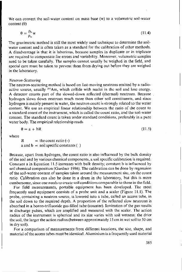
Tension Range O - 150 cm Undisturbed volumetric soil samples are placed upon a porous medium that is water- saturated (Figure 11.10). A water column of a certain length is then used to exert the desired suction or tension on the soil sample, via the porous medium. As the pore-size distribution of the soil influences its water-retaining properties, undisturbed soil samples have to be used. This method is called the ‘hanging water- column method’.

Tension Range 150 - 500 cm A slightly different procedure is used in this range, instead of a hanging water column, suction is created by a vacuum line connected to ceramic plates. The same volumetric samples are placed on these plates and water is drained from the samples until equilibrium with the plates is reached. This method is called the ‘suction plate method’.

40 1

pressure regulator

I soil sample

I

atmospheric 1 L porous compressor pressure ceramic plate

Figure 11.1 1 Measurement of the soil-water characteristic in the range of 15000 < h < -500 cm

Tension Range 500 - 15 O00 cm In the range of 500 to 15 O00 cm, instead of applying suctions, pressures are exerted on the soil sample, which is placed on a porous medium in a chamber (Figure 1 1.1 1). For pressures up to 3000 cm, undisturbed samples are normally used; for higher pressures, disturbed soil samples can be used. As porous medium, a ceramic plate or a cellophane membrane is used. Under the membrane, a shallow water layer under atmospheric pressure (zero gauge pressure) is present.

According to Equation 1 1.17, when he, is assumed to be zero,

h = h, + he,

Around the sample, the external imposed gas pressure is, say, 12 bar (i.e. equivalent to a head he, = 12 O00 cm). Water is discharged from the sample through the membrane into the water layer until equilibrium is reached. Then the pressure inside the soil sample is atmospheric, h = O. Hence, it follows that,

O = h, + 12000

or

h, = -12 O00 cm With this method, h,- 0 relationships can be determined over a large range of tensions. The method is referred to as the ‘pressure pan method’ for the lower range, when ceramic plates are used, and as the ‘pressure membrane method’ for higher pressures (Klute and Dinauer 1986).

In the very dry range, for h < -30 O00 cm (pF > 4 . 9 , the ‘vapour pressure method’ can be applied. For details, see Campbell and Gee (1986).

11.3.5 Drainable Porosity

The ‘storage coefficient’, p, also called ‘drainable pore space’, is important for unsteady drainage equations and for the calculation of groundwater recharge.

The storage coefficient is a constant that represents the average change in the water content of the soil profile when the watertable level changes with a discrete step. Its value depends on soil properties and the depth of the watertable. To derive a practical mean value of a storage coefficient for an area, it should be calculated for the major

402

soil series and for several depths of the watertable. If the water retention of the soil is known and if the pressure-head profile is known for two different watertable levels, the storage coefficient p can be calculated from the following equation

7.2 Z l

Usually, the drainable pore space is calculated for equilibrium conditions between soil-water content and watertable depth. The computer program CAPSEV (Section 1 1.4.2) offers the possibility of calculating the storage coefficient for different conditions with a shallow watertable. This could be useful information for the drainage of areas prone to high capillary rise.

In general, p increases with increasing watertable depths. The capillary reach in which equilibrium conditions exist is only active where the soil surface is nearby and when soil water is occasionally removed by evaporation. For a depth greater than a certain critical value (which depends on the soil type), the drainable porosity can be approximated by the difference in 8 between field capacity and saturation.

The concept of drainable porosity is shown in Figure 1 1.12A. In this figure, the soil-water content of a silty clay soil is shown by the line A-B for a watertable depth of 0.50 m, and by the line C-D for a watertable of 1.20 m. The drainable porosity in this case is represented by the enclosed area ABCD (representing the change in soil-water content), divided by the change in watertable depth AD or

I

(11.21)

where zI z2 8,(z) '= soil-water content as a function of soil depth for Watertable 1 (-) 8,(z) = soil-water content as a function of soil depth for Watertable 2 (-)

= watertable depth for Situation 1 (m) = watertable depth for Situation 2 (m)

ABCD p=- AD (1 1.22)

Example 11 .I Assume that the soil-water profile of Figure 11.12 is in equilibrium (i.e. H = O). Then, according to Equation 1 1.19, h = -2, with z = O at the watertable and positive upward. The pressure-head profile in this.case is simply -z. Pressure-head profiles for the two watertable depths are illustrated in Figure 11.12B. The soil-water content can now be determined graphically for each depth from the soil-water retention curve in Figure 1 1.12C. The calculations are presented in Table 1 1.2.

We divide the soil profile in discrete depth intervals of 0.10 m, and calculate the average difference in 8 between the first and the second watertable for each interval. This average is multiplied by the interval depth, which yields the water content per interval, totalling 28.05 mm. We divide the total by 700 mm (i.e. the change in watertable depth), and find a drainable porosity p = 0.04.

403

S @ P

depth in cm O

20

40

60

80

1 O0

120

140 I 0.40 0.45 0.50 0.55 0.60

water content O in cm3icm3

O O -20 -40 -60 -80 -100 -120 o 0.1 0.2 0.3 0.4 0.5 0.6

volumetric soil water content O in cm3icm3 oresure head in cm

Figure 11.12 A. Soil-water-content profiles for equilibrium conditions with the watertable at 0.50 m, O,(z), and at 1.20 m, e,(z). The area enclosed by 8, (z), 8, (2). the soil surface, and AD represents the drainable porosity

B. Equilibrium pressure-head profiles for watertables at 0.50 and 1.20 m C. Soil-water retention for a silty clay

Table 11.2 Calculation of the drainable porosity in a silty clay for a drop in watertable depth from 0.50 m to 1.201-11

Depth Heightabove pF = &(z) Heightabove pF = O,@) A8 = Average Average below soil wntenahle 1 log@,) wnteflnhle 2 IogfiJ 8,-8, A0 A8 surface, z h, = -z h, = -z X I 0 0

' The flow of soil water is caused by differences in hydraulic head, as was explained in Chapter 7, where water flow in saturated soil (i.e. groundwater flow) was discussed. The following sections deal with the basic relationships that govern soil-water flow in the unsaturated zone, the most important properties that influence soil-water dynamics, and some methods of measuring those properties.

' ~

(cm) (CI11) (-) (cm) (-1 (-) (mm)

O 50 1.70 0.476 120 2.08 0.459 0.017 IO 40 1.60 0.479 110 2.04 0.461 0.018 0.0175 1.75 20 30 1.48 0.483 1 O0 2.00 0.463 0.020 0.0190 1.90 30 20 1.30 0.847 90 1.95 0.466 0.021 0.0205 2.05 40 10 1.00 0.492 80 1.90 0.468 0.024 0.0225 2.25 50 O - m 0 s 70 1.85 0.470 0.307 0.0305 3.05 60 0.507 60 1.78 0.473 0.034 0.0355 3.55 70 0.507 50 1.70 0.476 0.031 0.0325 3.25 80 0.507 40 1.60 0.479 0.028 0.0295 2.95 90 0.507 30 1.48 0.483 0.024 0.0260 2.60

I O0 0.507 20 1.30 0.487 0.020 0.0220 2.20 110 0.507 IO 1.00 0.492 0.015 0.0175 1.75 I20 0.507 O - m " 0 . 0 0 7 5 0 . 7 5

Total 0.289 0.2805 28.05

28.05 700

p = ~ = 0.04

11.4 Unsaturated Flow of Water

11.4.1 Basic Relationships

Kinetics of Flow: Darcy's Law For the one-dimensional flow of water in both saturated and unsaturated soil, Darcy's Law applies, which can be written as

(1 1.23) q = - KVH

where q = discharge per unit area or flux density (m/d) K = hydraulic conductivity (m/d) H = hydraulic head (m) V = differential operator (V = d/ax + a/ay + d/az) (see also Chapter 7)

i 405

It was only in 1927 that Israelsen noticed that the equation for flow in unsaturated media presented by Buckingham in 1907 is equivalent to Darcy’s Law, the only difference being that the hydraulic conductivity is dependent on the soil-water content, which we denote as K(0). With the hydraulic head defined as in Equation 11.19, Darcy’s Law for unsaturated soils may be written as

(1 1.24)

(1 1.25)

(1 1.26)

where q,, qy, and qz are the components of soil-water flux in the x-, y- and z-directions.

Conservation of Mass: Continuity Equation In Chapter 7 (Section 7.3.3), a general form of the continuity equation was derived for water flow independent of time, considering the mass balance of an elementary volume that could not gain or lose water. In unsaturated soil, however, a similar elementary volume can gain water at the expense of air. If we state that this happens at a rate ae/at, we can write Equation 7.9 in the following form

(11.27)

General Unsaturated-Flow Equation The general equation of water flow in isotropic media (i.e. media for which the hydraulic conductivity is the same in every direction) is obtained by substituting Darcy’s Law (Equations 11.24, 11.25, and 11.26) into the continuity equation (Equation 1 1.27), which yields

(11.28)

or

= V.K(B) VH (11.29)

For saturated flow, the water content does not change with time (ignoring the compressibility of water and soil), so that ae/at = O, and hence

V.KVH = O (11.30)

If K is constant in space, the Laplace Equation for steady-state saturated flow in a homogeneous, isotropic porous medium follows from Equation 1 1.30

V2H = O (1 1.31)

V2 = Laplace Operator (see also Chapter 7, Section 7.6.5)

at

where

406

Substituting H = z + h into Equation 11.28 yields

(11.32)

Since 8 is related to h via the soil-water retention curve, we can also express K(0) as K(h) (see following section). Through the introduction of the specific water capacity, C(h), Equation 11.32 may be converted into an equation with one dependent variable

(1 1.33)

where C(h) = specific water capacity, equalling de/dh (i.e. the slope of soil-water

retention curve) (m-I)

Replacing K(8) by K(h) and substituting Equation 11.33 into Equation 11.32 yields

aK(h) (1 1.34) C(h) - ah = - a (K(h) g) + $(K(h) $) + & (K(h) E) + at ax

Equation 11.34 is known as Richards’ Equation. With p/pg substituted for h, this equation applies to saturated as well as to unsaturated flow (hysteresis excluded). To solve Equation 1 1.34, we need to specify the hydraulic-conductivity relationship, K(h), and the soil-water characteristic, 8(h). When we consider flow in a horizontal direction only (x), Equation 11.34 reduces to an equation for unsteady horizontal flow

Similarly, the equation for unsteady vertical flow is

(11.35)

(11.36)

ae at For steady-state flow, - = O and h is only a function of z. Hence Equation 11.36

reduces to

dz [ K(h) ($ + l)] = O (1 1.37)

(Section 11.4.2 will deal with steady-state flow in more detail.)

For transient (i.e. unsteady) flow, we find the commonly used one-dimensional equation by substituting Equation 11.33 into Equation 11.36, which yields

ah 1 a - - -- at - C(h) dz [K(h) ($ + ‘)I (1 1.38)

Equation 1 1.38 provides the basis for predicting transient soil-water movement in layered soils, each layer of which may have different physical properties.

407

11.4.2 Steady-State Flow

The most simple flow case is that of steady-state vertical flow (Equation 11.37). Integration of this equation yields

K(h) - + 1 = C (2 ) where c is the integration constant, with qz = x. Rewriting yields

where q K(h) = hydraulic conductivity as a function of h (m/d) h = pressurehead(m) z

= vertical flux density (m/d)

= gravitational potential, positive in upward direction (m)

Rearranging Equation 1 1.40 yields

(11.39)

(1 1.40)

(11.41)

K(h) To calculate the pressure-head distribution (i.e. the relationship between z and h for a certain K(h)-relationship and a specified flux q), Equation 1 1.41 should be integrated

(1 1.42)

where h, = the pressure head (m); the upper boundary condition z, = the height of capillary rise for flux q (m)

To calculate at what height above the watertable pressure head h, occurs, integration should be performed from h = O, at the groundwater level, to h,. When the soil profile concerned is heterogeneous, integration is performed for each layer separately

where N = the number of layers in the soil profile h,, h,, ..., hN = the pressure heads at the top of Layer 1,2 ,..., N

Solving Equation 11.43 yields the height of capillary rise, z, for given flux densities. The h-values at the boundaries between the layers are unknown initially, and must

be determined during the integration procedure. Thus, starting from h = O and z = O at the watertable, we steadily decrease h until z reaches zi, the known position

408

of the i-th boundary.. Since pressure head is continuous across the boundary (as opposed to water content), the value hi may be used as the lower limit of the next integration term. In this way, the integration proceeds until either the last value of h (hN) is reached or until z reaches the soil surface.

Equations 11.42 and 11.43 may be solved analytically for some simple K(h)- relationships. For more complicated K(h)-relationships, it would be very laborious, if not impossible, to find an analytical solution. Therefore, integration as described by Equations 11.42 and 11.43 is usually performed numerically, as, for example, in the computer program CAPSEV (Wesseling 1991).

For a marine clay soil in The Netherlands, the results of calculations with CAPSEV are shown in Figures 1 1.13A and 1 1.13B. Figure 1 1.13A shows the height of capillary rise and the pressure-head profile for different vertical-flux densities. Figure 1 1.13B shows the pressure-head profile during infiltration for several values of the vertical-flux density. The height of capillary rise was calculated for a watertable at a depth of 2 m. The soil profile consisted of five layers with differing soil-physical parameters.

1 I

j ,

Example 11.2 For drainage purposes, it can be useful to know the maximum flux for a given watertable pressure head and a certain watertable depth. Suppose that we have a crop

,

2 in cm above watertable

2 in cm above watertable

sand.. , . . .,.; . . . . . . , . . . . . . . . . . . .

o - I I I I I i I 1 I I I I I 1 1 1

loo lo1 lo2 l o3 lo4 lo5 O pressure head in cm

. . . . . . . . . . . . . . . . . . . . . . . . . . . . . . :::sand ' ::. . . . . . . . . . . . . . . . . . . . . . . . . . . . . . . . . . . . . . . . . . . . . . . . . . . . . . . . . . . . . . . . . . . . . . . O I 1 i I I

1 O0 200 300 pressure head in cm

Figure 11.13 Calculations with computer program CAPSEV for a 5-layered soil profile (Wesseling 1991) A. Height of capillary rise B. Pressure-head profiles in case of infiltration

409

which, on the average, is transpiring at a rate of 2 mm/d. This water is withdrawn from the rootzone, say from the top 0.20 m of the soil profile. We assume that the crop would suffer from drought if the pressure head in the centre of the rootzone were to fall below -200 cm. We further assume that the groundwater level can be fully controlled by drainage. To prevent drought stress for the crop under any condition, the controlled groundwater depth should be such that, under steady-state conditions with a pressure head of -200 cm at 0.10 m depth (i.e. the average depth of the rootzone), the water delivery from the groundwater by capillary rise would equal water uptake by the roots, equalling 2 mm/d.

We can find the required groundwater depth from Figure 1 1.13A. We start on the horizontal axis at a pressure head of -200 cm, draw an imaginary upward line until it crosses the 2 mm/d flux-density curve, then go horizontally to the vertical axis and find a depth of 0.86 m. This means that the desired watertable depth is 0.86 + 0.10 = 0.96 m below the soil surface.

11.4.3 Unsteady-State Flow

To obtain a solution for the unsteady-state equation (Equation 11.38), appropriate initial and boundary conditions need to be specified. As initial condition (at t = O), the pressure head or the soil-water content must be specified as a function of depth

h(z,t=O) = h, (11.44)

The boundary conditions at the soil surface (z = O) and at the bottom of the soil profile (z = -zN) can be of three types (see also section 1 1.8.2): - Dirichlet condition: specification of the pressure head; - Neumann condition: specification of the derivative of the pressure head, in

combination with the hydraulic conductivity K, which means a specification of the flux through the boundaries;

- Cauchy condition: the bottom flux is dependent on other conditions( e.g. an external drainage system).

This list is not exhaustive, while also, depending on the type of problem to be solved, boundary conditions can be defined by combinations of the above options. Equation 1 1.38 is a non-linear partial differential equation because the parameters K(h) and C(h) depend on the actual solution of h(z,t). The non-linearity causes problems in its solution. Analytical solutions are known for special cases only (Lomen and Warrick 1978). Most practical field problems can only be solved by numerical methods (Feddes et al. 1988). (Numerical methods used in the modelling of soil-water dynamics will be discussed in Section 1 1.8.)

11.5 Unsaturated Hydraulic Conductivity

The single most important parameter affecting water movement in the unsaturated zone is the unsaturated hydraulic conductivity, K, which appears in the unsaturated flow equation (Equation 11.38). In the case of saturated flow in soil, the total pore

410

space is filled with water and is thus available for flow. During unsaturated flow, however, part of the pores are filled with air and do not participate in the flow. The unsaturated hydraulic conductivity, K(8) or K(h), is therefore lower than the saturated conductivity. Thus, with decreasing soil-water content, the area available for flow decreases and, consequently, the unsaturated hydraulic conductivity decreases. The K in unsaturated soils depends on the soil-water content, 8, and, because 8 = f(h), on the pressure head, h. Figure 11.14 shows examples of K(8)-relationships for four layers of a sandy soil with a humic topsoil, together with the soil-water retention characteristics (De Jong and Kabat 1990).

Over the years, many laboratory and field methods have been developed to measure Kas a function of h or 8. These methods can be divided into direct and indirect methods (Van Genuchten et al. 1989). Direct methods are, almost without exception, difficult to implement, especially under field conditions. Despite a number of improvements, direct-measurement technology has only marginally advanced over the last decades.

Nevertheless, indirect methods, which predict the hydraulic properties from more easily measured data (e.g. soil-water retention and particle-size distribution), have received comparatively little attention. This is unfortunate because these indirect methods, which we call ‘predictive estimating methods’, can provide reasonable estimates of hydraulic soil properties with considerably less effort and expense. Hydraulic conductivities determined with estimating methods may well be accurate enough for a variety of applications (Wasten and Van Genuchten 1988). Other important indirect methods are inverse methods of parameter estimates with analytical models that describe water retention and hydraulic conductivity (Kabat and Hack-ten Broeke 1989).

pressure head in cm -lo5

4 -10

3 -10

2 -10

-10

- 1

log K i n m l d

O 0.1 0.2 0.3 0.4 0.5 volumetric soil water content

Figure I I . 14 Soil-water retention, h(B), and hydraulic conductivity, K(B), curves for four layers of a sandy soil (after De Jong and Kabat 1990)

41 1

11.5.1 Direct Methods

Comprehensive overviews of direct methods of measuring the unsaturated hydraulic conductivity, K, and the soil-water diffusivity (D), D = K(O>/(dO/dh), are given by Klute and Dirksen (1986) for laboratory methods, and by Green et al. (1 986) for field methods.

In the steady-state methods, the flux, q, and hydraulic gradient, dH/dz, are measured in a system of time-invariant one-dimensional flow, and the Darcy Equation (Equation 1 1.40) is used to calculate K. The value of K obtained is then related to a measured h or 8. The procedure can be applied to a series of steady-state flow situations.

Transient laboratory methods include the method developed by Bruce and Klute (1956), in which the diffusivity is estimated from horizontal water content distributions, and the sorptivity method of Dirksen (1975).

The most common field methods include the ‘instantaneous profile method’, a good example of which is described by Hillel et al. (1972). In this method, an isolated, free- draining field is saturated and subsequently drained by gravity, while the field is covered to prevent evaporation. The hydraulic conductivity is calculated by applying Darcy’s Law to frequent measurements of pressure head and water content during the drying phase. Various simplifications of this instantaneous profile concept, based on unit-gradient (dH/dz = 1, H = h + z, so h = constant, see Equation 11.37) approaches, have been developed (e.g. Libardi et al. 1980). This unit gradient does not require pressure-head measurements. These methods provide the hydraulic soil properties between saturation and field capacity, since gravity drainage becomes negligible at water contents below field capacity.

Clothier and White (1981) developed a method to determine K(8), 8(h), and D(8) from sorptivity measurements. ‘Sorptivity’ is the initial infiltration rate during the infiltration process. It can be measured quickly and is therefore a practical method of determining the hydraulic soil properties.

The ‘crust method’ of Bouma et al. (1971) is a field variant of steady state laboratory approaches. A soil column is isolated from the surrounding soil, covered with a crust, and a constant head is maintained on the crust. Because the hydraulic conductivity of the crust is relatively small compared with that of the soil, the pressure head in the soil will be lower than zero. Because a constant head is maintained above the crust, a steady-state flow will develop in the crust and a steady-state flux, lower than the saturated flux of the soil, will enter the soil and create a steady-state unsaturated flow. Hydraulic conductivities for different pressure heads can be determined with crusts of different material and thickness. The method allows us to determine hydraulic conductivities in the h-range of O to -100 cm.

All the above methods of measuring K(B), K(h), or D(8) are typically based on Darcy’s Law, or on various numerical approximations or simplifications of Equation 11.38. This enables us to express K or D in terms of directly observable parameters. These direct methods are relatively simple in concept, but they also have a number of limitations which restrict their practical use. Most methods are time-consuming because restrictive initial and boundary conditions need to be imposed (e.g. free drainage of an initially saturated soil profile). This is especially problematic under field conditions where, because of the natural variability in properties and the

412

uncontrolled conditions, accurate implementation of boundary conditions may be difficult.

Even more difficult are the methods requiring repeated steady-state flow or other equilibrium conditions. Many of the simplified methods require the governing flow equations to be linearized or otherwise approximated to allow their direct inversion, which may introduce errors. A final shortcoming of the direct methods is that they usually lack information about uncertainty in estimated soil hydraulic conductivity, because it is impractical to repeat the measurements a number of times.

A laboratory method which is more or less a transition between direct and indirect methods is the ‘evaporation method’ (Boels et al. 1978). In this method, an initially wet soil sample is subjected to free evaporation. The sample, 80 mm high and 100 mm in diameter, is equipped with four tensiometers. The sample is weighed at brief time intervals and, at the same time, the pressure head is recorded. From these weight and pressure-head data, the average soil-water retention at each time interval can be determined. An iterative procedure is now used to derive the soil-water retention, and the instantaneous profile method to derive the hydraulic conductivity for each depth interval of 20 mm around a tensiometer. In this way, the method yields soil-water retention and hydraulic conductivity for h = -100 to -800 cm for sandy soils and for h = -20 to -800 cm for clay soils.

The advantages of the evaporation method are that it simultaneously yields both soil-water retention and hydraulic conductivity over a relatively wide h-range. The experimental conditions, in terms of boundary conditions, are close to natural conditions, because water is removed by evaporation. Disadvantages are that the procedure takes a considerable time (approximately 1 month per series of samples), and that the soil-water retention and hydraulic conductivity are based on an iterative procedure.

11.5.2 Indirect Estimating Techniques

Many of the disadvantages of the direct techniques do not apply to the indirect techniques. The indirect methods can basically be divided into two categories: ‘predictive estimates’ and ‘parameter estimates’. The advantage of both methods is that neither depends on the created ideal experimental conditions.

The usefulness of predictive estimates depends on the reliability of the correlation or transfer function, and on the availability and accuracy of the easily measured soil data. The estimate functions are often called ‘pedo-transfer functions’ because they transfer measured soil data from one soil to another, using pedological characteristics.

The parameter-estimate approach for soil hydraulic properties is based on inverse modelling of soil water flow. This approach is very flexible in boundary and initial conditions. The inverse approach was developed parallel with advances in computer and software engineering (Feddes et al. 1993a).

Prediction of the K(h) Function from Soil Texture and Additional Soil Properties The methods discussed in this section are referred to as ‘pedo-transfer functions’. Pedo- transfer functions are usually based on statistical correlations between hydraulic soil properties, particle-size distribution, and other soil data, such as bulk density, clay

41 3

mineralogy, cation exchange capacity, and organic carbon content. Other pedo- transfer functions relate parameters of the Van Genuchten model (see the following section) in a multiple regression analysis to, for example, bulk density, texture, and organic-matter content (e.g. Wösten and Van Genuchten 1988).

The development of pedo-transfer functions offers promising prospects for estimating soil hydraulic properties over large areas without extensive measuring programs. Such pedo-transfer functions are only applicable to areas with roughly the same parent material and with comparable soil-forming processes. Developing and testing these methods is as yet far from complete. Vereecken et al. (1992), for example, concluded that errors in estimated soil-water flow were more affected by inaccuracies in the pedo-transfer functions than by errors in the easily measured soil characteristics.

Another approach to identifying hydraulic soil properties on a regional scale is by identifying 'functional soil physical horizons'. This approach was followed by Wösten ( 1 987), who used measured values of soil-water retention and hydraulic conductivity of representative Dutch soils, and classified these in groups according to texture and position in the soil profile. These groups were called functional soil physical horizons. Another example is the Catalogue of Hydraulic Properties of the Soil by Mualem (1976a).

Predicting the K(h) Function from Soil- Water Retention Data The most simple form of parameter estimating concerns the prediction of K(h) from soil-water retention data. Water retention is more easily measured than hydraulic conductivity, and the estimating methods are usually based on statistical pore-size distribution models (Mualem 1976b). The most frequently applied predictive conductivity models are those of Mualem and Burdine (Van Genuchten et al. 1989). Van Genuchten (1980) combined Mualem's model with an empirical S-shaped curve for the soil-water retention function to derive a closed-form analytical expression for the unsaturated hydraulic conductivity curve.

The empirical Van Genuchten Equation for the soil-water retention curve reads

(1 1.45)

where 0, = residual soil-water content (i.e. the soil water that is not bound by

capillary forces, when the pressure head becomes indefinitely small) (-) 8, = saturated soil-water content (-) a = shape parameter, approximately equal to the reciprocal of the air-entry

'n = dimensionless shape parameter (-) m = 1-l/n

value (m-I)

After combining Equation 11.45 with the Mualem model, we find the Van Genuchten- Mualem analytical function, which describes the unsaturated hydraulic conductivity as a function of soil-water pressure head

[l - IClhl"-l ( 1 + Ic~~I")"]~ [l + lahlnImh K(h) = K,

414

(1 1.46)

where K, = saturated hydraulic conductivity (m/d) h = a shape parameter depending on dK/dh

The shape parameters in Equations 1 1.45 and 1 1.46 can be fitted to measured water- retention data. The Van Genuchten model in its most free form contains six unknowns: €4, 0,, ct, n, h, and K,. Although, with specially developed computer programs, the mathematical fitting procedure enables us to find these unknowns for measured data, its use as a predictive model in this form is difficult. The fitting procedure is improved when some measurable parameters are known approximately, so that they can be optimized in a narrow range around these measured values.

To predict K(h) from the water-retention curve, we need to measure K,. However, if a few K(h)-values are known in combination with soil-water-retention values, K, can be found with an iteration procedure and need not be measured. Computer software has been developed (Van Genuchten et al. 1991) to fit the analytical functions of the model to some measured 0(h) and K(h)-data. The same program allows the K(h)-function to be predicted from observed water-retention data.

Yates et al. (1992) recently evaluated parameter estimates with different data sets and for various combinations of known and unknown parameters. They concluded that predicting the unsaturated hydraulic conductivity from soil-water retention data and measured K,-values yielded poor results. Using a simultaneous fitting of K(h) and 0(h) data, while treating h as an unknown parameter, improved results significantly. Apparently, water-retention data combined with a measured K, are not always sufficient to describe the K(h)-function with Equation 11.46.

The Van Genuchten model in,its original form is inadequate for very detailed simulation studies, because it is only valid for monotonic wetting or drying. By adding only one parameter, Kool and Parker (1987) extended the model so as to include hysteresis in O(h) and K(h) functions.

Inverse Problem combined with Parameter Optimization Techniques In this approach, the direct flow problem can be formulated for any set of initial and boundary conditions and solved with an analytical or numerical method. Input data are measured soil-water contents, measured pressure-head profiles, or measured discharge under known boundary conditions, or any combination thereof, always as a function of time. Certain constitutive functions for the hydraulic properties are assumed, and unknown parameter values in those functions are estimated with the use of an optimization procedure. This optimization minimizes the objective function (e.g. the sum of the squared differences between observed and calculated values of either water content or pressure head) until a desired accuracy is reached.

The inverse method can be applied to both laboratory experiments and field experiments. A disadvantage of the laboratory procedure is that we cannot explore the full potential of this method, because of the necessarily limited size of the soil sample. Moreover, the collection of soil samples always introduces some disturbance that may affect flow properties. Thus, applying the method in-situ seems to offer the best prospects. The capabilities of this technique have been shown by Feddes et al. (1993a and b) and Kool et al. (1987).

415

11.6 Water Extraction by Plant Roots

Under steady-state conditions, water flow through the soil-root-stem-leaf pathway can be described by an analogue of Ohm's Law with the following widely accepted expression

(1 1.47)

where T = transpiration rate (mm/d) h,,h,,h, = matric heads in the soil, at the root surface, and in the leaves,

Rs,R, respectively (mm)

= liquid flow resistances in soil and plant, respectively (d)

If we consider the diffusion of water towards a single root, we can see that R, is dependent on root geometry, rooting length, and the hydraulic conductivity of the soil. This so-called microscopic approach is often used when evaluating the influence of complex soil-root geometries on water and nutrient uptake under steady-state laboratory conditions. In the field, the components of this microscopic approach are difficult to quantify for a number of reasons. Steady-state conditions hardly exist in the field. The living root system is dynamic, roots grow and die, soil-root geometry is time-dependent, and water permeability varies with position along the root and with time. Root water uptake is most effective in young root material, but the length of young roots is not directly related to the total root length. The experimental evaluation of root properties is difficult, and often impossible.

Although detailed studies can be relevant for a better understanding of plant physiological processes, they are not yet usable in describing soil-water flow. Thus, instead of considering water flow to single roots, we follow a macroscopic approach. In this approach, a sink term, S, is introduced, which represents water extraction by a homogeneous and isotropic element of the root system, and added to the continuity equation (Equation 11.27) for vertical flow (Feddes et al. 1988)

(1 1.48)

Consequently, the one-dimensional equation for transient soil-water movement (Equation 11.38) can be rewritten as

where S = sink term (d-I)

(1 1.49)

The sink term, S, is quantitatively important since the water uptake can easily be more than half of the total change in water storage in the rootzone over a growing season.

Feddes et al. (1988), in the interest of practicality, assumed a homogeneous root distribution over the soil profile and defined S,,, according to

s,,, = L I L I ZA

416

(11.50)

where S,,, = the maximum possible water extraction by roots (d-') T, = the potential transpiration rate (mm/d) (Z,( = the depth of the rootzone (mm)

I O

Prasad (1988) introduced an equation to take care of the fact that, in a moist soil, the roots principally extract water from the upper soil layers, leaving the deeper layers relatively untouched. He assumed that root water uptake at the bottom of the rootzone equals zero and derived the following equation

S,,,(Z) = - 1 - - 2T IZrI ( 13 (1 1.51)

Both root water-uptake functions are shown in Figure 1 1.15.

So far, we have considered root water uptake under optimum soil-water conditions (i.e. S,J. Under non-optimum conditions, when the rootzone is either too dry or too wet, S,,, is dependent on (h) and can be described as (Feddes et al. 1988)

S(h) = 4h)Smax (1 1.52)

a(h) = dimensionless, plant-specific prescribed function of the pressure head where

The shape of this function is shown in Figure 11.16. Water uptake below Ih,l (oxygen deficiency) and above Ih,l (wilting point) is set equal to zero. Between Ih,l and Ih31 (reduction point), water uptake is at its maximum. Between lhll and lh21, a linear relation is assumed, and between Ih,l and /h41, a linear or hyperbolic relation between u and h is assumed. The value of Ih,l depends on the evaporative demand of the atmosphere and thus varies with T,.

S U S

z = z, z = z,

Figure 11.15 Different water-uptake functions under optimum soil-water conditions, S,,,, as a function of depth, z, over the depth of the rootzone, zr, as proposed by A: Feddes et al. (1988) and B: Prasad (1988)

417

a 1 .o

0.8

0.6

0.4

0.2

0.0 h4

pressure head, h

Figure 11.16 Dimensionless sink-term variable, a, as a function of the absolute value of the pressure head, h (after Feddes et al. 1988)

11.7 Preferential Flow

In the previous sections, we described unsaturated-zone dynamics for isotropic and homogeneous soils. The fact that most soils are neither was already recognized in the 19th century. In natural soils, the transport of water is often heterogeneous, with part of the infiltrating water travelling faster than the average wetting front. This has important theoretical and practical consequences. Theoretical calculations of the field water balance, the derived crop water use, and the estimated crop yield are incorrect if preferential flow occurs but is not incorporated. Practically, preferential flow has a strong impact on solute transport and on the pollution of groundwater and subsoil (e.g. Bouma 1992). Preferential flow varies considerably from soil to soil, in both quantity and intensity. In some soils, preferential flow occurs through large pores in an unsaturated soil matrix, a process known as ‘by-pass flow’ or ‘short-circuiting’ (Hoogmoed and Bouma 1980). In other soils, flow rates vary more gradually, making it difficult to distinguish matrix and preferential pathways.

Preferential flow of water through unsaturated soil can have different causes, one of them being the occurrence of non-capillary-sized macropores (Beven and Germann 1982). This type of macroporosity can be caused by shrinking and cracking of the soil, by plant roots, by soil fauna, or by tillage operations. Wetting-front instability, as caused by air entrapment ahead of the wetting front or by water repellency of the soil (Hendrickx et al. 1988) can also be viewed as an expression of preferential flow. Whatever the cause, the result is that the basic partial differential equations (Equations 11.38 and 1 1.49) describing water flow in the soil need to be adapted.

Hoogmoed and Bouma (1 980) developed a method of calculating infiltration, including preferential flow, into clay soils with shrinkage cracks. The method combines vertical and horizontal infiltration. It is physically based, but was only applied to soil cores of 200 mm height and was not tested in the field. Bronswijk (1991) introduced a method in which preferential flow through shrinkage cracks is calculated as a function of both the area of cracks at the soil surface, and the maximum infiltration rate of the soil matrix between the cracks.

The division of soil water over the soil matrix and the macropores, and the fate of water flowing downward through the macropores, is handled differently in the

418

variable crack vflume subsidence

lC2. T I E R . . . . . . . . .

. . . . . . . . . . . . .- - . . . . . . . . . . . . . . . . . . . . . . . . . . . . . . . . .-

_ _ _ -

- matrix - crack system at time t

matrix - crack system al time t + A I

Figure 11.17 Concept for unsaturated water transport in cracking soils. I is the infiltration rate into the soil matrix, I, is infiltration into cracks, I, is the horizontal flux through the walls of the macropores, q is the Darcy Flux between two nodal points, and qb is the bottom flux of the system (after Feddes et al. 1988)

various methods mentioned above. The common principle, however, is essentially the two-domain concept. The interaction between water in the two domains is also important. In some approaches, the total preferential flow is accumulated at the bottom of the macropores and is then added to the unsaturated flow at that depth (Bronswijk 1991).

A more general approach was suggested by Feddes et al. (1988), who linked preferential flow and matrix flow by extending the basic differential equation (Equation 1 1.49)

(1 1.53)

where B = source of soil water due to horizontal infiltration into the macropores,

or a sink due to evaporation through the walls of the macropores

The resulting model is schematically illustrated in Figure 1 1.17. The quantification of the B-term in Equation 11.53, however, is difficult and requires a number of simplifications (Bronswijk 199 1).

11.8 Simulation of Soil-Water Dynamics in Relation to Drainage

The design of drainage systems is usually based on criteria that are derived from steady- state or unsteady-state equations (Chapter 17). The underlying theories are mainly based on saturated flow to drains (Chapter 8), and do not consider the effects of drainage in the unsaturated zone, which is where the crops are rooted. The performance of drainage systems designed with those equations is subsequently tested

419

in field trials or pilot areas (Chapter 12). Because of budget and time constraints, pilot areas may not represent the complete range of environmental conditions in a project area, and may not give an insight into the long-term sustainability of the drainage project.

Computer modelling can therefore be an important source of additional information, because many project conditions can be simulated quickly and cheaply for various time intervals. The principles and processes presented in Sections 1 1.3 to 1 1.7 can be used to predict soil-water dynamics and crop response. The interactions between all components involved are described by mathematical relationships, which can be combined in simulation models. One such simulation model is SWACROP (Kabat et al. 1992), which allows the user to evaluate the effect of different drainage strategies (i.e. criteria and designs) on water conditions in the unsaturated rootzone, and hence on crop production. After some introductory explanations (Sections 11.8.1 to 1 1.8.3), we shall illustrate the modelling approach with a number of examples from water-management and drainage practice (Section 1 1.8.4).

11.8.1 Simulation Models

‘Simulation’ is the use of models as tools to imitate the real behaviour of existing or hypothesized systems. Most important and interesting is the simulation of dynamic systems. Simulation models are usually realized in the form of computer programs and are therefore also referred to as ‘computer models’.

A drainage simulation model for the unsaturated zone and crop production should, for example, be able to describe the effects of a specific drainage design on soil-water dynamics and related crop yields. Soil-water flow is also the governing factor in solute transport, and is thus responsible for changes in soil chemical status (e.g. plant nutrients and soil salinity; Chapter 15). Appropriate simulation models can predict the effects of different drainage designs on water and salt balances, which, in turn, relate to crop production.

The most complex simulation models are mathematical models that employ numerical techniques to solve differential equations (Section 11.8.2). Even if these models are mathematically and numerically correct, they need to be verified and calibrated against field data, and the required accuracy of input data needs to be assessed (Section 11 3.3).

11.8.2 Mathematical Models and Numerical Methods

Mathematical Models In the previous sections, soil-water dynamics were cast in the form of mathematical expressions that describe the hydrological relationships within the system. The set of relevant partial differential equations, together with auxiliary conditions, define the mathematical model. The auxiliary conditions must describe the system’s geometry, the system parameters, the boundary conditions and, in the case of transient flow, also the initial conditions.

If the governing equations and auxiliary conditions are simple, an exact analytical

420

solution may be found. Otherwise, a numerical approximation is needed. Numerical simulation models are by far the most common ones.

Numerical Methods At present, numerical approximations are possible for complex, compressible, non- homogeneous, and anisotropic flow regions having various boundary configurations.

Numerical methods are based on subdividing the flow region into finite segments bounded and represented by a series of nodal points at which a solution is sought. This point solution depends on the solutions of the surrounding segments, and also on an appropriate set of auxiliary conditions.

In recent years, a number of numerical methods have been introduced. The most appropriate methods for soil-water movement are 'finite-difference methods' and 'finite-element methods'.

To illustrate the use of finite-difference methods, we shall consider the case of one- dimensional unsaturated flow without sinks/sources (Equation 11.36). Let the flow depth be divided into equal intervals, AZ, and the time be similarly divided into time steps, At. The resulting two-dimensional grid is shown in Figure 1 I . 18.

Equation 11.36 can now be expressed in finite difference form as

where i = index along the space coordinate j = index along the time abscissa

Equation 1 1.54 represents the so-called forward difference scheme with an explicit linearization of the K(0)-function.

Z =

Figure 11.18 Bi-linear grid superimposed on the z-t-plane with the flow and time domain divided into equal intervals. The grid represents a forward finite difference scheme

42 1

Backward-difference schemes also exist: The resulting set of algebraic equations can be solved with special techniques such as linearization. The advantage of the finite- difference method is its simplicity and its efficiency in treating time derivatives. On the other hand, the method is rather incapable of dealing with complex geometries of flow regions, and has a few other drawbacks as well.

With finite-element methods, the flow area is divided into a number of rigid elements. In modelling soil-water flow problems, triangular elements can be efficiently used to represent difficult geometries and to be more precise in regions where rapid changes are expected (e.g. near the soil surface or wetting fronts). Figure 11.19 shows an example of such a triangular nodal network. The corners of the triangular elements are designated as nodal points. In these nodes, state variables like matric head are specified. Via a number of techniques, one first gets a set of quasi-linear first-order differential equations, which are then discretisized and integrated in discrete time steps. The resulting set of non-linear equations is then solved, until iterations have converged to a prescribed degree of accuracy.

Finite-element methods are capable of solving complex flow geometries, with non- linear and time-dependent boundary conditions, while possessing great flexibility in following rapid soil-water movement. In many cases, the rate of convergence of the finite-element methods exceeds that of the finite-difference methods. A drawback of the finite-element method is the rather time-consuming and laborious preparation of the solution mesh. With an automatic mesh generation model, however, this problem can be considerably reduced. Another problem is that checking the finite-element solution by simple calculations is not always possible.

Initial Conditions Initial conditions must be defined when transient soil-water flow is being modelled. Usually, values of matric head or soil-water content at each nodal point within the soil profile are required. When these data are not available, however, water contents at field capacity or those in equilibrium with the watertable might be regarded as the initial ones.

Upper Boundary Conditions While the potential evaporation rate from a soil depends only on atmospheric

I

Figure 11.19 Network of triangular finite elements. The corners of the element e are designed as nodal points n, in which state variables are located

422

conditions, the actual flux through the soil surface is limited by the ability of the soil matrix to transport water. Similarly, if the potential rate of infiltration exceeds the infiltration capacity of the soil, part-of the water is stored on the soil surface or runs off, because the actual flux through the top layer is limited by moisture conditions in the soil. Consequently, the exact upper boundary conditions at the soil surface cannot be estimated apriori, and solutions must be found by maximizing the absolute flux, as explained by Feddes et al. (1988).

Lower Boundary Conditions The lower boundary of the unsaturated zone is usually taken at the phreatic surface, except if the watertable is very deep, when an arbitrary lower boundary is set. Generally, one of the following lower boundary conditions are used: - Dirichlet condition: The main advantage of specifying a matric head zero as the

bottom boundary is that it is easy to record changes in the phreatic surface of a watertable. A drawback is that, with shallow watertables (< 2 m below soil surface), the simulated effects of changes in phreatic surface are extremely sensitive to variations in the soil’s hydraulic conductivity;

- Neumann condition: A flux as lower boundary condition is usually applied in cases where one can identify a no-flow boundary (e.g. an impermeable layer) or where free drainage occurs. With free drainage, the flux is always directed downward and the gradient dH/dz = 1, so the Darcian Flux is equal to the hydraulic conductivity at the lower boundary;

- Cauchy condition: This type of boundary condition is used when unsaturated flow. models are combined with models for regional groundwater flow or when the effects of surface-water management are to be simulated under conditions of surface or subsurface drainage (see Figure 11.20). Writing the lower boundary flux, qb, as a function of the phreatic surface, which in this case is the dependent variable, one can incorporate relationships between the flux to/from the drainage system and the height of the phreatic surface. This flux-head relationship can be obtained from drainage formulae such as those of Hooghoudt or Ernst (see Chapter 8) or from regional groundwater flow models (e.g. Van Bake1 1986).

With the lower boundary conditions, the connection with the saturated zone can be established. In this way, the effects of activities that influence the regional groundwater system upon, say, crop transpiration can be simulated. The coupling between the two systems is possible by regarding the phreatic surface as an internal moving boundary with one-way or two-way relationships.

The most general form of the Cauchy condition can be written as

qb = q d + qa (11.55)

where qb = the flux through the lower boundary (m/d) q d = the flux from/to the drainage system (m/d) qa = the flux to/from deep aquifers (m/d) (Figure 1 1.20)

When the Cauchy condition is linked with a one-dimensional vertical- flow model,

423

. . . . . . . . . . . . . . . . . . . . . . . . . . . . . . . . . . . . . . . . . . . . . . . . . . . . . . . . . . . . . . . . . . . . . . . . . . . . . .

. . . . . . . . . . . . . . . . . . . . . . . . . . . . . . . . . . . . . . . . . . . . . . . . . . . . . . . . . . . . . . . . . . . . . . . . . . . . . . . . . . . . . . . . . . . . . . . . . . . . . . . . . . . . . . . . . . . . . . . . . . . . . . . . . . . . . . . . . .

Figure 11.20 The flow situation (Cauchy lower boundary condition) for outflow from ditches and downward seepage to the deep aquifers: h, is the open water level; h2 is the phreatic surface level; h3is the level of the phreatic surface averaged over the area; and h4 is the piezometric level of the deep aquifer

one can regard such a solution as quasi-two-dimensional, since both vertical and horizontal flow are calculated.

11.8.3 Model Data Input

Required Input Data The simulation of water dynamics in the unsaturated zone requires input data on the model parameters, the geometry of the system, the boundary conditions, and, when transient flow is being simulated, initial conditions. The geometry parameters define the dimensions of the problem domain, while the physical parameters describe the physical properties of the system under consideration. Unsaturated-zone flow depends on the soil-water characteristic, 8(h), and the hydraulic conductivity, K(8). If root water uptake is also modelled, parameters defining the relationship between water uptake by the roots and soil-water tension should be given, together with crop specifications. If a functional flux-head relationship is used as lower boundary condition, the parameters describing the interaction between surface water and groundwater and - if necessary - the vertical resistance of poorly permeable layers have to be supplied.

Before the models can be used to simulate the effects of different drainage strategies on the unsaturated zone, the models need to be calibrated. This can be done by comparing the results of model simulations with measured data from special calibration fields, and by adapting appropriate parameter values within the plausible range until simulation results and field measurements correspond to the desired degree. The calibrated model subsequently needs to be validated on another data set which

424

was not used for the calibration. Only when calibration and val;idation are satisfactory can the model be applied to simulate the effects of drainage strategies for use in design procedures. A good calibration requires a profound analysis of the model parameters and of their influence on model results. (For details on model calibration, see specialized publications on this subject: e.g. Kabat et al. 1994).

Spatial Variability One of the issues that complicate model calibration is spatial variability of soil hydraulic parameters and related terms of the water balance.

Most models of the unsaturated zone are one-dimensional. The hydrological and drainage problems that have to be modelled, however, concern areas, and have a spatial component, be it a local or a regional one. If the area were to be homogeneous in all its components, a point simulation could be representative of an entire region. The soil, however, is never homogeneous, but is subject to spatial variability. The variability of a parameter will not only influence the measuring program, but is also important for evaluating possible model accuracies.

The basic assumption of spatial variability in the unsaturated zone is that the porous medium is a macroscopic continuum with properties that are continuous functions of the space coordinates. The description of spatial variability by statistical techniques is referred to as 'geostatistical methods' (e.g. Jury et al. 1987). Geostatistics can be used to determine the most efficient sampling schemes to obtain practical mean values of spatially dependent properties (e.g. soil hydraulic properties) within a specific soil or land unit. It can also be used to describe the variability of those properties and for the regionalization of point simulations. A proper application of the geostatistical approach may reveal field characteristics that are not apparent from conventional statistical analysis, but are not without significance for the properties being considered.

A frequently used technique to account for spatial variability is 'scaling'. Scaling can also be used to regionalize one-dimensional simulation models. In principle, scaling is a technique of expressing the statistical variability in, for instance, the hydraulic conductivity in functional relationships. By this simplification, the pattern of spatial variability is described by a set of scale factors, defined as the ratio between the characteristic phenomenon at the particular location and the corresponding phenomenon of a reference soil (Hopmans 1987).

Accuracy of Hydraulic Soil Parameters The reliability of the results of simulation depends on the reliability of the model and on the accuracy of the parameters used in the model. The reliability and accuracy of the model are assessed by calibration and validation.

The required accuracy of input data should be relevant to the type of application and the type of problem to be solved (Wösten et al. 1987). It is also a function of ,the scale of the problem and of the sensitivity of the process to the parameters used. "For site-specific studies, a higher accuracy is required than for regional studies. For processes directly dependent on the hydraulic soil properties (e.g. capillary rise, recharge to the groundwater, and solute transport), the required accuracy is higher than for processes that are related to the soil hydraulic properties in a more integrated way (e.g. seasonal crop transpiration or crop production).

425

Kabat and Hack-ten Broeke (1989) used the SWACROP simulation model to investigate the sensitivity of different land qualities to hydraulic soil parameters, using data collected for a maize crop over 1985 and 1986. Simulated pressure heads at 5 cm depth - a measure for the land qualities of workability and trafficability -were computed for three different K(8) relationships (Figure 11.21). From the data for both years, they concluded that the three unsaturated conductivities led to considerable differences in trafficability, especially during wet periods (h > -100 cm). It appears that K(8) needs to be known quite accurately for this direct land quality.

In contrast, the cumulative actual dry-matter-production curves, representing an integrated land.quality, showed no (1985) or only minor (1986) differences as a result of the different K(8)'s (Figure 11.21). This proves that the sensitivity to hydraulic soil parameters can decrease when more integrated land qualities are considered.

0.0 0.2 0.4 0.6 Volume soil water content (cm3.cm.3)

0 ~ " " ' " ' 140 160 180 200 220 240 260 280

20

- r

m r 4 15 - C ._ c

3 U

10 o c

E ? m 5

9

U

c

Time (Julian days)

Actual production 1985

--- K 101 2 - K ('3) 3

K (e) i

O 140 160 180 200 220 240 260 280

Time (Julian days)

-3000

-2500 I

E

Pressure head at 5 cm 1986

K ( 0 ) 1 K (Q) 2 K ( Q ) 3

_-- -

o - -2000 -

o 2=

E

140 160 180 200 220 240 260 280 Time (Julian days)

Actual production 1986

K (e) 1 --- K (0) 2

K ( Q ) 3 -

Time (Julian days)

Figure 11.21 Sensitivity of the SWACROP model to the soil hydraulic parameter K(0) in terms of pressure heads at 5 cm depth and actual dry-matter production (after Kabat and Hack-ten Broeke 1989)

426

11.8.4 Examples of Simulations for Drainage

Three examples of the application of the SWACROP simulation model in drainage problems will be given. Two of the examples concern water management under the moderate humid conditions of The Netherlands. The third concerns drainage and irrigation in the sub-tropical semi-arid conditions of Pakistan.

SWACROP (Kabat et al. 1992) describes transient water flow in a heterogeneous soil-root system, which can be under the influence of groundwater. It contains a crop- growth simulation routine, which describes the potential and actual crop production as a function of crop transpiration and of a few other environmental variables. Soil- water movement is simulated in response to pressure-head gradients according to Equation 11.49. Upper and lower boundary conditions can be set to reproduce a variety of common hydrological field situations. The model allows us to simulate subsurface and surface drainage systems, and irrigation.

Example 11.3 Drainage of Arable Land in The Netherlands An integrated simulation approach, based on the agrohydrological model SWACROP, was developed by Feddes and Van Wijk (1990). In the integrated approach, land capability is quantified in terms of crop productivity under different conditions of climate, soil, drainage or irrigation, and farm management. The model can consider the following aspects, all of which can be affected by the operation of a drainage system via the soil-water conditions in the unsaturated zone: - Number of days in spring when the soil-water content in the upper soil layer is

low enough to permit soil cultivation and sowing or planting (farm-management aspect);

- Germination and crop emergence related to soil-water content and soil temperature; - Water uptake, and growth and production of the crop between emergence and

- Number of workable days in autumn, when soil-moisture conditions allow harvest;

harvesting operations (farm-management aspect).

The model calculated the effects of 15 combinations of drain depth and spacing on the yield of potatoes and spring cereals grown over 30 years on eight major soil types in The Netherlands. Three different definitions of seasonal yield were introduced: Y,,,, the production under optimum water supply and earliest possible emergence; Ypot, which includes retardation due to excessive wetness (insufficient drainage); and Y,,,, representing for the actual water supply to account for the drainage effect on the yield:

(11.56)

The spring term, YpOt/Ymax, accounts for a reduction in crop yield as a result of retarded planting and emergence. The growing season term, Yact/Ypot, quantifies the effects of too dry conditions (i.e. when the system is ‘over-drained’ and there are water shortages in the rootzone), or too wet conditions (when the system is ‘under-drained’) on the crop yield. The overall drainage effect, Yac,/Ymax, is the product of these two ratios.

We shall use the analysis of Feddes and Van Wijk (1990) and look at the yield of potatoes. For each of the eight major soil types in this study, the water-retention

427

G3 relative yield

@ relative yield

1 .o0

0.95

0.90

0.85

0.80 I I I I I 60 90 120 150 180

drain depth in cm below surface

0.40 ' I I I I 60 90 120 150 180

drain depth in cm below surface

o relative vield

actual yield per ha

1 .o0

0.90

0.80

0.70

drain depth in cm below surface

15

14

13

12

11

10

9

8

7

6

Figure 11.22 Drainage effects on potato yield based on a 30-year simulation for eight major soil types (Numbers 1-8) in relation to drain depth (after Feddes andVan Wijk 1990) A. Decrease in relative yield due to too wet soil conditions and delayed workability and emergence in spring; B. Decrease in relative yield due to moisture shortage during the growing season; C. Reduction in total relative yield, the combined effect of too wet soil conditions in spring and water shortage during the growing season

and hydraulic-conductivity characteristics were determined in the laboratory. The soils were: ( I ) a humus sand, (2) loamy sand, (3) peaty sand, (4) silty loam, (5) sandy loam, (6) loam, (7) silty clay loam, and (8) silty clay.

Figure 1 1.22A shows the effect of drain depth on the spring-reduced relative yield Yp,,/Y,,, , averaged over the 30 simulated years. The most severe yield deficits occur at drain depths of 0.6 and 0.9 m in the sandy and loamy soils (Soils 1 to 5). The reductions are less pronounced for the loam soil (6), and almost absent for the clay soils (7-8). To avoid any risk of sub-optimum yields due to late planting on all soils, this simulation would lead to a recommended drain depth of 1.5 - I .8 m.

Figure 1 1.22B shows the effect of drainage during the growing season on relative yield, YaCt/Ypot. Yields are now decreasing with greater drain depths. This points to a general ‘over-draining’ for depths greater than 0.9 m. The greatest damage due to over-draining occurs on the peaty sand (3). Apart from the humus sand (I), which also seems somewhat susceptible to drought, the other soils show only a slight response to drain depth during the growing season.

Figure 11.22C shows the combined effect of drainage on the yield of the potatoes. We can draw the following conclusions: - The optimum drainage depth depends strongly on the soil type. It varies from about

0.9 m for peaty sand (3) to about 1.3 - 1.4 m for sandy loam (5); - The effect of soil wetness is most pronounced for the loamy sand (2) and sandy

loam (5). Increasing the drain depth from 0.6 m to between 0.9 m and 1.2 m leads to a relative yield increase of the order of 10% for these soils. They have the highest unsaturated hydraulic conductivity under wet conditions and are characterized by an abrupt decrease in conductivity below a certain soil-water content upon drying. During wet conditions, they are thus subject to the largest capillary supply from the watertable (see Section 11.4.2);

- Heavier soils (6, 7, and 8) have a lower hydraulic conductivity and hence their response to increasing drainage depth is less pronounced;

- Except for the peaty sand (3), the effect of a too dry soil on overall drainage benefits is very small for drainage depths between 1.2 and 1.8 m.

The results of this study were used as the basis for a nationwide system to evaluate the effects of soil and.drainage upon crop yields.

Example 11.4 Water Supply Plan in an Area with Surface Drainage The economic feasibility of expanding the water supply for agriculture in a region in the north-eastern part of The Netherlands was investigated with the use of a special version of SWACROP (Werkgroep TUS-IO-PLAN 1988; Van Bake1 1986). The region is intensively drained through a multiple-level canal system (Figure 1 1.23).

Figure 11.23 schematically shows that the water level in the main canals can be regulated via inlet and outlet structures. Water levels in the tertiary canals can be regulated in the same way. These tertiary canals drain the fields during the wet season. During the dry season, the inlet water infiltrates into the soil and creates better soil- water conditions in the rootzone (i.e. in the unsaturated zone) (see also Figure 11.20).

The region was divided into about 200 different combinations of soil type, hydrological properties, and land use. Each of these sets was modelled with the special version of SWACROP, which was extended with a module for manipulating the water

429

level in (drainage) canals. The effects upon' actual transpiration of the water supply through drainage canals (sub-irrigation), combined with supplementary sprinkler irrigation, were caiculated for each set, using meteorological data for the years

Since actual transpiration is related to soil-water conditions by a water-uptake function (as was explained in Section 1 1.6), the simulation of unsaturated-zone dynamics played a major role in this study. The simulation results (i.e. crop yield and other agricultural benefits) were expressed in monetary terms. On this basis, areas that would benefit from a water supply through the existing system of drainage canals could be located. Different degrees of such benefits could even be distinguished (Figure 11.24).

1954- 1983.

Example 11.5 Drainage to Combat Waterlogging and Salinity in Pakistan Boers et al. (1993) used simulation model SWATRE (which is the soil-water component of SWACROP) to calculate the best drainage design for an irrigated area in the Indus Plains of Pakistan. The area is characterized by a subtropical semi-arid climate, with hot summers and cool winters, and monsoon rainfall, with high inter- annual variability. Major problems in the area are a high watertable that frequently hampers crop production, and secondary soil salinity.

The authors calibrated the model on a representative field in the area. The upper boundary conditions were potential crop evaporation, and rainfall and irrigation data. The lower boundary conditions were the watertable depth and the existing drainage design. The discharge to drains was calculated according to the Hooghoudt Equation (Chapter 8). The calibration was done by using different sets of independently measured hydraulic soil properties and by varying the correction factor for bare soil evaporation. The model was considered calibrated when weekly measured soil-water tensions at O. 15 m intervals over a depth of 0-2.0 m corresponded almost completely with the simulated ones for two consecutive years.

The calibrated model was subsequently used to calculate actual transpiration and (de)salinization for different drain depths and widths. The calculations were performed for a low-rainfall year, a moderate-rainfall year, and a high-rainfall year, selected from the climatic records of a nearby meteorological station. The objective of the model calculations was to maximize actual crop transpiration (as a measure of yield) and to mimimize the accumulation of salts in the rootzone.

The results indicated that the prevention of waterlogging during a wet monsoon was the most critical condition. Control of soil salinity appeared to be less critical.

Although these results are preliminary, the example shows that the simulation of water flow in unsaturated soils is capable of evaluating the influence of drainage design on vital conditions for crop production in areas prone to a combination of salinization and waterlogging.

43 1

References

Bertuzzi, P., L. Bruckler, Y . Gabilly and J.C. Gaudu 1987. Calibration, field testing, and error analysis

Beven, K. and P. Germann 1982. Macropores and water flow in soils. Water Resour. Res., 5, pp. 131 1-1325. Boek, D., J.B.H.M. van Gils, G.J. Veerman and K.E. Wit 1978. Theory and system of automatic

determination of soil moisture characteristics and unsaturated hydraulic conductivities. Soil Sci., 126,

Boers, Th. M., J. Beekma, Z.I. Raza and T.J. Kelleners 1993. Use of SWATRE in an irrigated field of the Indus Plains, Pakistan. Transactions of the 2nd ICID workshop on crop water models : water balance, crop water use and production. The Hague, September 1993. Winand Staring Centre.

Bouma, J. 1992. Influence of soil macroporosity on environmental quality. Advances in Agronomy 46. Academic Press, pp. 1-37.

Bouma, J., D.I. Hillel, F.D. Hole and C.R. Amerman 1971. Field measurement of hydraulic conductivity by infiltration through artificial crusts. Soil Sci. Soc. Am. Proc., 35, pp. 362-364.

Bronswijk, J.J.B. 1991. Magnitude, modeling and significance of swelling and shrinkage processes in clay soils. Thesis, Agricultural University Wageningen, 145 p.

Bruce, R.R. and A. Klute 1956. The measurements of soil moisture diffusivity. Soil Sci. Soc. Am. Proc.

Bruckler, L. and J.C. Gaudu 1984. Use of the micropsychrometers for soil water potential measurements in the laboratory or in the field. Agronomy, 4,2, pp. 171-182.

Campbell, G.S. and G.W. Gee 1986. Water potential: miscellaneous methods. In: A. Klute and R.C. Dinauer (eds.), Methods of soil analysis. 2nd ed. Part 1. Agronomy 9-1. American Society of Agronomy, Madison, pp. 493-544.

Cassel, D.K. and D.R. Nielsen 1986. Field capacity and available water capacity. In: A. Klute and R.C. Dinauer (eds.), Methods of soil analysis. 2nd ed. Part 1. Agronomy 9- 1. American Society of Agronomy, Madison, pp. 493-544.

Clothier, B.E. and I. White 1981. Measurement of sorptivity and soil water diffusivity in the field. Soil Sci. Soc. Am. J., 45, pp. 241-245.

De Jong, R. and P. Kabat 1990. Modelling water balance and grass production. Soil Sci. Soc. Am. J.,

Dean, T.J., J.P. Bell and A.J.B. Baty 1987. Soil moisture measurements by an improved capacitance technique. Part I. Sensor design and performance. J. of Hydrol., 93, pp. 67-78.

Dirksen, C. 1975. Determination of soil water diffusivity by sorptivity measurements. Soil Sci. Soc. Am. Proc., 39, pp. 22-27.

Feddes, R.A., P. Kabat. P.J.T. van Bakel, J.J.B. Bronswijk and J.M. Halbertsma 1988. Modelling soil water dynamics in the unsaturated zone state of the art. J. of Hydrol., 100, pp. 69-1 11.

Feddes, R.A. and A.L.M. van Wijk 1990. Dynamic land capability model : a case history. Philosophical Transaction Royal Society London, B 329, pp. 41 1-419.

Feddes, R.A., M. Menenti, P. Kabat and W.G.M. Bastiaansen 1993a. Is large scale inverse modelling of unsaturated flow with areal average evaporation and surface soil moisture from remote sensing feasible? J. of Hydrol., 143, pp. 125-152.

Feddes, R.A., G.H. Rooij, J.C. van Dam, P. Kabat, P. Droogers and J.N.M. Stricker 1993b. Estimation of regional effective hydraulic parameters by inverse modelling. In: D. Ruso and G. Dagan (eds.), Water flow and solute transport in soils : modelling and applications. Springer Verlag, Berlin, pp. 21 1-23 1.

Gardner, H. 1986. Water content. In: A. Klute and R.C. Dinauer (eds.), Methods of soil analysis. Part 1. Agronomy 9-1. American Society of Agronomy, Madison, pp. 493-544.

Green, R.E., L.R. Ahuja and S.K. Chong 1986. Hydraulic conductivity, diffusivity and sorptivity of unsaturated soils : field methods. In: A. Klute and R.C. Dinauer (eds.), Methods of soil analysis. 2nd ed. Part I . Agronomy 9.1. American Society of Agronomy, Madison, pp. 771-798.

Gurr, C.G. and B. Jakobsen 1978. Gamma probe for measurement of field bulk density and water content. In: W.W. Emerson, R.O. Bond and A.R. Dexter (eds), Modification of soil structure. Wiley, Chichester,

Halbertsma, J.M., C. Przybyla and A. Jacobs 1987. Application and accuracy of a dielectric soil water content meter. Proc. Int. Conf. Measurement of Soil and Plant Water Status, Logan, Vol. I , pp. 11-1 5 .

Heimovaara, T.J. and W. Bouten 1990. A computer-controlled 36-channel time domain reflectometry system for monitoring soil water contents. Water Res. Res., 26, pp. 231 1-2316.

of a gamma-ray probe for in situ measurement of dry bulk density. Soil Sci., 144,6, pp. 425-436.

pp. 191-199.

20, pp. 458-462.

54, pp. 1725-1732.

pp. 127-133.

432

Hendrickx, J.M.H., L.W. Dekker, M.H. Bannink and H.C. Van Ommen 1988. Significance of soil survey for agrohydrological studies. Agric. Water Manage., 14, 1/4, pp. 195-208.

Hilhorst, M.A. 1984. A sensor for determination of the complex permittivity of materials as a measure for moisture content. In: P. Bergveld (ed.), Sensors and actuators. Twente University of Technology, Enschede, pp. 79-84.

Hilhorst, M.A. 1986. Device for measuring moisture tension of a substrate. European patent pending no. 86202367.

Hillel, D., V.D. Krentos and Y . Stylianou 1972. Procedure and test of an internal drainage method for measuring soil hydraulic characteristics in situ. Soil Sci., 1 14, pp. 395-400.

Hoogmoed, W.B. and J. Bouma 1980. A simulation model for predicting infiltration into cracked clay soil. Soil Sci. Soc. Am. J., 44, pp. 458-461.

Hopmans, J.W. 1987. A comparison of various methods to scale soil hydraulic properties. J. of Hydrol.,

Jury, W.D., D. Russo, G. Sposito and H. Elabo 1987. The spatial variability of water and solute transport properties in unsaturated soil. I. Analysis of property variation and spatial structure with statistical models. Hilgardia 55, 4, pp. 1-32.

Kabat, P. and M.J.D. Hack-ten Broeke 1989. Input data for agrohydrological simulation models : some parameter estimation techniques. In: H.A.J. van Lanen and A.K. Bregt (eds.), Application of computerized EC soil map and climate data. Commission of the European Communities, Report EUR

Kabat, P., B.J. van den Broek and R.A. Feddes 1992. SWACROP : A water management and crop production simulation model. ICID bulletin, 41,2, pp. 61-84.

Kabat, P., B. Marshall and B.J. van den Broek 1994. Comparisons of the parameterization and calibration scheme’s related to the performance of the models. In: Kabat et al. (ed.): Modelling of water dynamics, evaporation and plant growth with special reference to potato crop. Wageningen Press, 450 p.

Klute, A. and R.C. Dinauer (eds.) 1986. Methods of soil analysis. Part I. 2nd ed. Agronomy 9-1, American Society Agronomy, Madison, I182 p.

Klute, A. and C. Dirksen 1986. Hydraulic conductivity and diffusivity : laboratory methods. In: A. KIute and R.C. Dinauer (eds.), Methods of soil analysis, Part I . 2nd ed. Agronomy 9-1. American Society Agronomy, Madison, pp. 687-734.

Kool, J.B. and J.C. Parker 1987. Development and evaluation of closed-form expressions for hysteretic soil hydraulic properties. Water Resour. Res., 23, 1, pp. 105-1 14.

Kool, J.B., J.C. Parker and M.Th. van Genuchten 1987. Parameter estimation for unsaturated flow model: a review. J. Hydrol. 91, pp. 255-293.

Libardi, P.L., K. Reichardt, D.R. Nielsen and J.W. Biggar 1980. Simple field methods for estimating soil hydraulic conductivity. Soil Sci. Soc. Am. J., 44, pp. 3-7.

Lomen, D.O. and A.W. Warrick 1978. Time-dependent solutions to the one-dimensional linearized moisture flow equation with water extraction. J. Hydrol., 39, 1-2, pp. 59-67.

Mualem, Y . 1976a. A catalogue of the hydraulic properties of soils. Project 442. Institute of Technology, Haifa.

Mualem, Y. 1976b. A new model for predicting the hydraulic conductivity of unsaturated porous media. Water Resour. Res., 12, pp. 513-522.

Phene, C.J., Ch.P. Alle and J. Pierro 1987. Measurement of soil matric potential and real time irrigation scheduling. In: W.R. Gardner (ed.), Proceedings International Conference on measurements of soil and plant water status, Utah State University, Logan, pp. 258-265.

93,314, pp. 241-256.

12039 EN, pp. 45-62.

Prasad, R. 1988. A linear root water uptake model. J. Hydrol., 99, pp. 297-306. Topp, G.C., Davis, J.L. and A.P. Annan 1980. Electromagnetic determination of soil water content :

measurements in coaxial transmission lines. Water Resour. Res., 16, pp. 574-582. Topp, G.C. and Davis, J.L. 1985. Measurement of soil water using time-domain reflectometry (TDR) :

field evaluation. Soil Sci. Soc. Am. J., 49, pp. 19-24. Van Bakel, P.J.T. 1986. A systematic approach to improve the planning, design and opearation of regional

surface water management systems: a case study. Institute Land and Water Management Research, Report 13, Wageningen, 118 p.

Van den Elsen, H.G.M. and J.W. Bakker 1992. A universal device to measure the pressure head for laboratory use or long-term stand-alone field use. Soil Sci., 154,6, pp. 458-464.

Van Genuchten, M. Th. 1980. A closed-form equation for predicting the hydraulic conductivity of unsaturated soils. Soil Sci. Am. J., 44, pp. 892-898.

i 433

Van Genuchten, M.Th., F. Kaveh, W.B. Russel and S.R. Yates 1989. Direct and indirect methods for estimating the hydraulic properties of unsaturated soils. In: J. Bouma and A.K. Bregt (eds.), Land qualities in space and time. PUDOC, Wageningen, pp. 61-73.

Van Genuchten, M.Th., F.J. Leij and S.R. Yates 1991. The RETC code for quantifying the hydraulic functions of unsaturated soils. U.S. Environmental Protection Agency, ADA, EPA/600/2-91/065,85 p.

Vereecken, H., J. Diels, J. Orshoven , J. Bouma 1992. Functional evaluation of pedotransfer functions for the estimation ofsoil hydraulic properties. Soil Sci. Soc. Am. J., 56,5, pp. 1371-1378.

Wesseling, J.G. 1991. CAPSEV : steady state moisture flow theory, program description and user manual. Winand Staring Centre, Report 37, Wageningen, 5 1 p.

Werkgroep TUS-IO-PLAN 1988. Water voor Drenthe. Rapport van de werkgroep TUS- IO-PLAN, Provinciaal Bestuur van Drenthe, Assen, 101 p.

Wösten, J.H.M. 1987. Beschrijving van de waterretentie- en doorlatenheids-karakteristieken uit de Staringreeks met analytische functies. Rapport Stichting voor Bodemkartering, 2019, Wageningen, 54 p.

Wösten, J.H.M., M.H. Bannink and J. Bouma 1987. Land evaluation at different scales : you pay for what you get. Soil Surv. Land Eva]., 7, pp. 13-14.

Wösten, J.H.M. and M.Th. van Genuchten 1988. Using texture and other soil properties to predict the unsaturated soil hydraulic functions. Soil Sci. Soc. Am. J., 52, pp. 1762-1770.

Yates, S.R., M.Th. Van Genuchten, A.W. Warrick and F.J. Leij 1992. Analysis of measured, predicted and estimated hydraulic conductivity using the RETC computer program. Soil Sci. Soc. Am. J., 56, pp. 347-354.

434