
1.1 Historical Developments of Fiber Optic...
43
Introduction to Fiber Optic Sensors and Fiber Gratings 1 1.1 Historical Developments of Fiber Optic Sensors Through a long process of evolution, the development of human society has now entered a highly information-oriented era. The information technology has become the major trend of contemporary development. With more and more high technology products going into peoples’ lives, there is more demand for high-speed and large- capacity information carriers. These have been the targets for many researchers. In past forty years, revolution is brought out in information technology due to developments in optoelectronics and telecommunication industries. Improvements in quality and cost reduction in optoelectronic components led the industry to bring out high performing devices such as compact disc, players, bar code scanner, high end lasers, laser printers, CCD camera, LCD projector, stable photodiodes, high sensitive photodetectors, phototransistors, etc. Ultra fast development in telecommunication was due to developments in fiber optics communication industry by providing high performance and more reliable telecommunication links, larger bandwidth for information carriage at low cost. The invention of lasers in 1960’s opened new window for researchers to study the optical fibers for data communication, sensing and other applications in the next decade. Researchers conducted experiments by transmitting the laser beam in different waveguides. In the beginning large losses in optical fibers prevented the replacement of co-axial cables by optical fibers. Early fibers had losses of 1000dB/km, means only 1% of light transmitted in 20m fiber, making them impractical in communication use. Charles Kao who won Nobel Prize in 2009 for his contributions along with his co-worker G. A. Hockham investigated fundamental properties of optical fibers in detail way back in 1966 for optical communication and came to conclusion that – the losses in dielectric media were mostly caused by
Transcript of 1.1 Historical Developments of Fiber Optic...

Introduction to Fiber Optic Sensors and Fiber Gratings
1
1.1 Historical Developments of Fiber Optic Sensors
Through a long process of evolution, the development of human society has now
entered a highly information-oriented era. The information technology has become
the major trend of contemporary development. With more and more high technology
products going into peoples’ lives, there is more demand for high-speed and large-
capacity information carriers. These have been the targets for many researchers. In
past forty years, revolution is brought out in information technology due to
developments in optoelectronics and telecommunication industries. Improvements in
quality and cost reduction in optoelectronic components led the industry to bring out
high performing devices such as compact disc, players, bar code scanner, high end
lasers, laser printers, CCD camera, LCD projector, stable photodiodes, high sensitive
photodetectors, phototransistors, etc. Ultra fast development in telecommunication
was due to developments in fiber optics communication industry by providing high
performance and more reliable telecommunication links, larger bandwidth for
information carriage at low cost.
The invention of lasers in 1960’s opened new window for researchers to study the
optical fibers for data communication, sensing and other applications in the next
decade. Researchers conducted experiments by transmitting the laser beam in
different waveguides. In the beginning large losses in optical fibers prevented the
replacement of co-axial cables by optical fibers. Early fibers had losses of
1000dB/km, means only 1% of light transmitted in 20m fiber, making them
impractical in communication use. Charles Kao who won Nobel Prize in 2009 for his
contributions along with his co-worker G. A. Hockham investigated fundamental
properties of optical fibers in detail way back in 1966 for optical communication and
came to conclusion that – the losses in dielectric media were mostly caused by

Introduction to Fiber Optic Sensors and Fiber Gratings
2
absorption and scattering. The latter was predominantly caused by impurities, in
particular iron ions present. Fibers with glass of higher purity could be a good
candidate for optical communication. As coated by C. Kao - “Compared with existing
coaxial cable and radio systems, this form of waveguide has a larger information
capacity and possible advantages in basic material cost. The realization of a
successful fiber waveguide depends, at present, on the availability of suitable low-loss
dielectric material. The crucial material problem appears to be one which is difficult
but not impossible. Certainly, the required loss figure of around 20dB/km is much
higher than the lower limit of loss figure imposed by the fundamental mechanisms ,”
[1]. Later in 1969 C. Kao along with other co-workers, showed that fused silica (SiO2)
had purity for good optical communication. An intense worldwide research with aim
to produce low loss optical fibers began. In 1970, research team from the Corning
Glass Works in the United States consisting of F. P. Kapron, D. B. Keck, P. C.
Schultz, F. Zimar, under the leadership of R. D. Maurer, succeeded in making glass
fibers of fused silica with low losses as C. Kao had envisioned. The team fabricated
fiber by chemical method called chemical vapor deposition (CVD). To make a core
and cladding with very close refractive indices, they doped titanium in the fused silica
core and used pure fused silica in the cladding. A few years later (in 1974), loss even
reached 4dB/km at 850nm using germanium instead of titanium. Several other
technologies were developed in Japan, USA and UK. In that direction J. B.
MacChesney and co-workers at Bell Laboratories developed a modified CVD
technique, allowing efficient production of optical fibers. Within a few years,
attenuation less than 1dB/km was achieved, which was even far below the target set
by C. Kao. Today, attenuation of light around 1.55µm wavelength in fibers is below
0.2dB/km [2]. Modern optical fibers are extraordinarily transparent media, with more
Introduction to Fiber Optic Sensors and Fiber Gratings
3
than 95% light transmitted after 1km propagation [3]. Later advances in fiber optic
technology have significantly changed the telecommunication industry. The ability to
carry gigabits of information at the speed of light increased the research potential in
optical fibers. Improvements and cost reductions in optoelectronic components led to
emergence of new product area.
With improved technologies of manufacturing, optical fiber material loss almost
disappeared and the sensitivity for detection of the losses increased. With
development in low power measurement detectors, one could even sense small
changes in phase, intensity and wavelength of a light carried by an optical fiber due to
outside perturbations on the fiber. Optical fiber being physical medium is subjected to
perturbation of one or the other kind. Therefore it experiences geometrical (size,
shape, strain) or optical (RI, mode conversion) changes depending upon the nature
and magnitude of the perturbation. In telecommunication applications, one tries to
minimize such effects so that signal transmission and reception is reliable. On the
other hand, in fiber optic sensor (FOS) field, the response to external perturbation is
deliberately enhanced, so that the resulting change in optical radiation can be used as
measure of external perturbation. In FOS, the fiber acts as modulator. It also serves as
transducer and converts measurement data like temperature, stress, strain, rotation or
electrical and magnetic currents into corresponding change in optical radiation. This
sub branch of optical fiber technology soon saw an intense R&D activities around the
world, which led to the emergence of the new field called ‘Fiber Optic Sensors’.
Development of optical fiber sensors started in 1977 even though some isolated
demonstrations were made in earlier days. Many laboratories entered into the field
resulting into rapid progress. In the beginning fiber optics sensors were developed for
sensing sound [4-6], pressure [7-9], temperature [10], magnetic field [11, 12], rotation

Introduction to Fiber Optic Sensors and Fiber Gratings
4
[13, 14], current [15, 16], acceleration, fluid level, torque, photo acoustics, current,
displacement etc [17].
Light is characterized by phase, polarization, frequency, wavelength and intensity
(amplitude). Any one or more of these parameters may undergo a change due to
external perturbation. Our ability to measure and quantify the change reliably and
accurately is state of art of sensor design. In fiber optic sensors, information is
conveyed by change either in phase, polarization, frequency, wavelength, intensity or
combination of above properties of optical fiber. But the potodetector, being
semiconductor device only senses the intensity of light at the detector surface. Hence,
the art of sensing with phase, frequency or polarization modulation involves
interferometric or grating based signal processing optical circuits.
1.2 Advantages of Fiber Optic Sensors
The main drive of research in FOS area today is to produce a range of optical-
fiber based techniques which can be used to measure different physical parameters,
providing a foundation for an effective measurement technology, strengthen the
technology that can compete with conventional methods and tackling difficult
measurement situations where conventional sensors are not well suited to use in a
particular environment. The resulting sensors have a series of characteristics those are
significantly advantageous compared to conventional electrical sensors. Following are
some advantages of FOS compared to conventional electrical sensors. Following are
some advantages of FOS compared to conventional electrical sensors [18].
1. Sensed signal is immune to electromagnetic interference (EMF) and radio
frequency interference (RFI).
2. Intrinsically safe in explosive environments.

Introduction to Fiber Optic Sensors and Fiber Gratings
5
3. Highly reliable and secure with no risk of fire /spark.
4. High voltage insulation and absence of ground loops and hence avoid any
necessity of isolation devices like optocouplers.
5. Low volume and light weight (1kilometer of 200µm silica fiber weighs only
70grams and occupies volume of nearly 30cm3).
6. As point sensors, they can be used to sense parameters in inaccessible regions
without perturbation of the transmitted signals.
7. They be easily interfaced with low-loss optical fiber telemetry and hence
affords remote sensing by locating the control electronics for LED/lasers and
detectors far away from the sensor head.
8. Large bandwidth and hence offer possible multiplexing a large number of
individually addressed point sensors in a fiber network or distributed sensing.
9. Chemically inert and they can be readily employed in chemical processes and
biomedical instrumentation due to their smaller size and mechanical
flexibility.
10. Multifunctional sensing capabilities such as strain, pressure, corrosion,
temperature and acoustic signals.
11. Robust, more resistant to harsh environments.
These advantages were sufficient to attract intensive research and development
activities around the world to develop new class of sensors based on fiber optics.
This has eventually led to the emergence of variety of fiber optic sensors for accurate
sensing and measurement of physical parameters [18].
Some of the disadvantages of FOS were also noticed during different sensor
developments. One is the poor elastic property that makes optical fiber extremely
brittle. This is not particularly desired for sensing applications. Consequently, the
Introduction to Fiber Optic Sensors and Fiber Gratings
6
handling, treatment and operation of FOS require extreme care. In addition, each
process requires technical skills. With the current technology, in situ assembly of the
optical system is a cumbersome and exhaustive process, since the measurement setup
of the optical fiber sensor system is comprised of different modules (for example,
light source, coupler and receiver), difficult splicing process and the constant need
for careful treatment. Although the method of manufacturing fiber gratings has
improved considerably, current technology only manages to produce one at one time
and most of the process still requires manual handling. In addition, the cost of
running fiber grating writing facilities is high due to expensive laser, masks (both
phase mask and amplitude masks) and the requirement for a highly skilled operator.
The lifespan of optical fiber is considered long for telecommunications, between 20
to 25 years, it may be not enough for some of sensing applications. Typical civil
engineering structures such as buildings, bridges and dams typically have lifespan of
more than 70 years where FOS is used for structural health monitoring. Therefore,
packaging FOS is next big task after a sensor design [19-23].
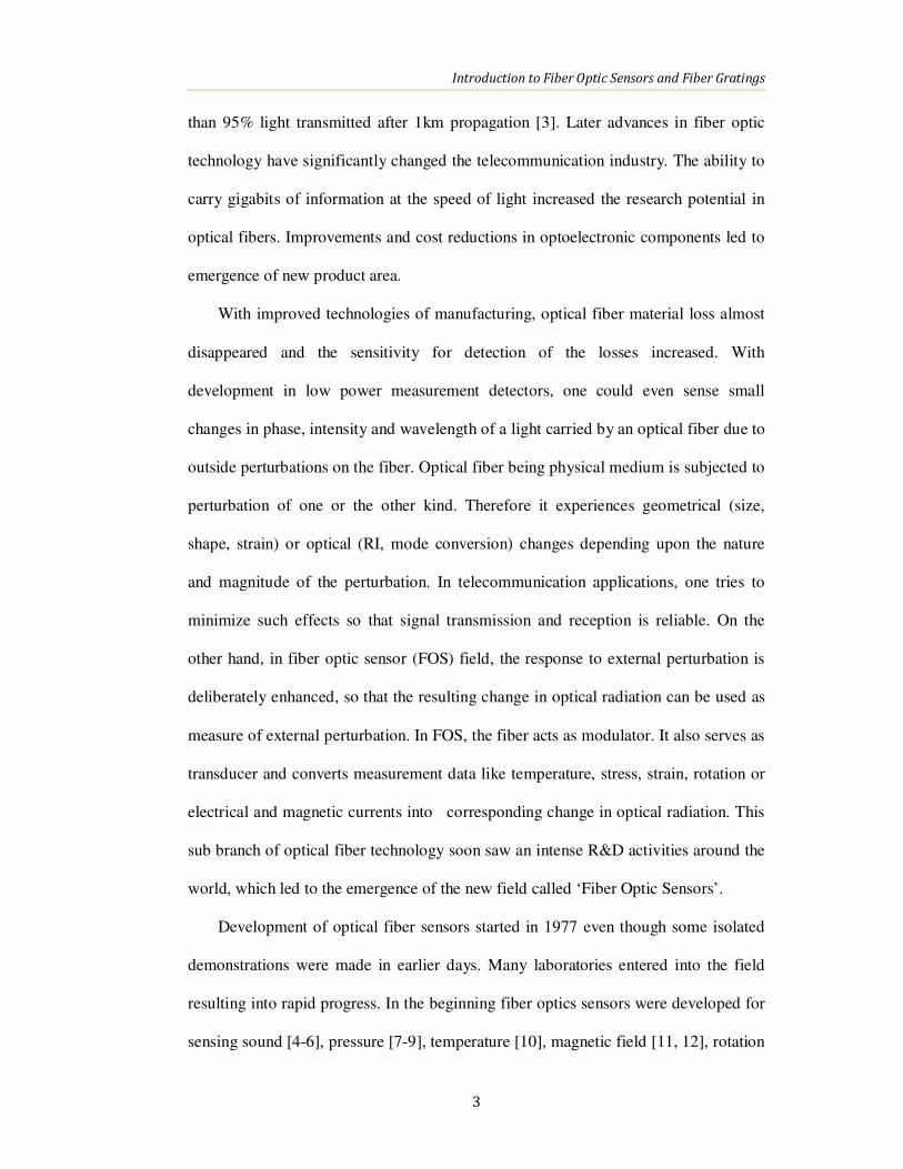
1.3 Basic Principle of Fiber Optic Sensor
Although light is trapped within the dielectric medium of the optical waveguide,
the radiation that propagates inside the waveguide can be perturbed by the external
environment and this perturbation can be used to draw useful information for sensing
purposes. In fact, the interaction of the physical parameter of interest that is measured
with the waveguide produces a modulation in the propagation constants of the guided
light beam. This modulation is a sensitive function of the measurand of interest.
Following are basic elements constituting a fiber optic sensor [19-21].
Introduction to Fiber Optic Sensors and Fiber Gratings
7
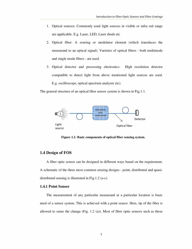
1. Optical sources: Commonly used light sources in visible or infra red range
are applicable. E.g. Laser, LED, Laser diode etc
2. Optical fiber: A sensing or modulator element (which transduces the
measurand to an optical signal). Varieties of optical fibers - both multimode
and single mode fibers - are used.
3. Optical detector and processing electronics: High resolution detector
compatible to detect light from above mentioned light sources are used.
E.g. oscilloscope, optical spectrum analyzer etc).
The general structure of an optical fiber sensor system is shown in Fig.1.1.
Figure 1.1: Basic components of optical fiber sensing system.
1.4 Design of FOS
A fiber optic sensor can be designed in different ways based on the requirement.
A schematic of the three most common sensing designs - point, distributed and quasi-
distributed sensing is illustrated in Fig.1.2 (a-c).
1.4.1 Point Sensor
The measurement of any particular measurand at a particular location is basic
need of a sensor system. This is achieved with a point sensor. Here, tip of the fiber is
allowed to sense the change (Fig. 1.2 (a)). Most of fiber optic sensors such as those
Detector
Light
source
Interaction
with
measurand
Optical fiber

Introduction to Fiber Optic Sensors and Fiber Gratings
8
used in the monitoring of temperature, acceleration, pressure or chemical parameters
use this design [22].
1.4.2 Distributed Sensor
With some sensors, the whole length of the fiber can be used as a sensing
element. The measurand action is sensed along the length of the fiber itself and
process is termed distributed sensing, illustrated in Fig. 1.2(b). This principle has been
employed widely in the measurement of temperature using non-linear effects in fibers,
such as Brillouin or Raman scattering or in some types of strain sensing. This yields
either an enhanced sensitivity if the fiber is wrapped up to form a single sensing point
or it can be used for spatial averaging of the signal [22].
1.4.3 Quasi Distributed Sensor
A style of sensor that is somewhat in between these two types of sensors is
termed quasi-distributed. As shown schematically in Fig. 1.2(c), the measurand
information is obtained at different pre-determined points along the length of a fiber
network. Here, the fiber has been sensitized or special materials have been introduced
into the fiber loop to allow the measurement to be taken and this technique has been
applied to temperature and chemical sensing, e.g., using different fiber types [22]
Figure 1.2: Scheme of three most common fiber optic sensor designs: (a) Point sensor,
(b) Distributed Sensor, (c) Quasi distributed sensor.
Light source,
detection &
signal
processing
Light
sourceDetection &
signal
processing
Light
source
Detection &
signal
processing
(a) (b) (c)

Introduction to Fiber Optic Sensors and Fiber Gratings
9
1.5 Types of Fiber Optic Sensors
Varieties of fiber optic sensors were developed in the direction to full fill the
needs of human society. Optical fiber sensors are classified into different classes
based on different categories: the sensing location, the operating principle, the
applications etc [18, 20].
1.5.1 Based on Sensing Location
In FOS, the light may be modulated either inside or outside the optical fiber i.e.
sensing location may be inside or outside the fiber. Hence, based on sensing location
FOSs are classified broadly as intrinsic and extrinsic sensors. This is the simplest
classification of fiber optic sensors.
1.5.1.2 Intrinsic Sensor
In intrinsic fiber optic sensor, the interaction occurs within an element of optical
fiber itself and light never leaves the waveguide. External environment acts on the
fiber and the fiber in turn changes some characteristic of the light inside the fiber that
is measured using the detector. One or more of the physical properties of the guided
light, e.g., intensity, phase, polarization or wavelength is modulated by the
measurand. A schematic illustration of intrinsic sensor can be seen in Fig. 1.3.
Examples for intrinsic sensors are pressure sensor, temperature sensor, strain sensor,
etc. [18, 20, 23, 25].
Fiber Optic Sensor
Intrinsic Sensor Extrinsic Sensor

Introduction to Fiber Optic Sensors and Fiber Gratings
10
Figure 1.3: Intrinsic sensor illustration.
1.5.1.2 Extrinsic Sensor
In extrinsic fiber optic sensor, the optical fiber is used to couple light, usually to
and from the region where the light beam is influenced by the measurand (or external
environment). In this case, the fiber just acts as a means of getting the light to the
sensing location and to detector as shown in Fig 1.4. Common examples of this type
of sensors are optical fiber endoscopy, displacement sensor and fiber-optic
fluorescence sensor. In fiber-optic fluorescence sensor the light is coupled out of the
fiber and excites the analyte. The light emitted by fluorescence of the analyte is
collected by the second fiber and guided to the detector [18-21].
Figure 1.4: Extrinsic sensor illustration.
1.5.2 Based on Modulation Technique
Based on the operating principle or modulation and demodulation process, a fiber
optic sensor can be classified into 4 groups
1. Intensity modulated sensor
2. Wavelength modulated sensor
Light
Source Detector
Feed
Fiber
Receiver
fiber
Action

Introduction to Fiber Optic Sensors and Fiber Gratings
11
3. Polarization modulated sensor
4. Phase modulated sensor
All these parameters may be subject to change due to external perturbations. Thus, by
detecting these parameters and their changes, the external perturbations can be sensed
1.5.2.1 Intensity Modulated Sensor
Intensity modulation is simplest and cheapest method of detecting different
parameters using optical fiber. Intensity-based fiber optic sensors are based on
intensity undergoing change. In intensity modulated fiber optic sensors, measurand
modulates the intensity of light transmitted through the optical fiber and variations in
the intensity are measured at the output end of the optical fiber using a detector.
Intensity modulated sensors are analogue in nature and have significant usage in
digital applications for switches and counters [23]. These require more light and
therefore usually use multimode optical fibers. Intensity modulated FOS can be found
in variety of intrinsic and extrinsic configurations. The intensity modulation can be
achieved through variety of methods or mechanisms such as transmissive, reflective,
microbending, attenuation and evanescent fields that can produce a measurand
induced change in the optical intensity propagated by an optical fiber [23].
The advantages of these sensors are: Simplicity of implementation, low cost,
possibility of being multiplexed and ability to perform as real distributed sensors. The
drawbacks are: Relative measurements and variations in the intensity of the light
source may lead to false readings, unless a reference system is used [20].
1.5.2.2 Wavelength Modulated Sensors
Wavelength modulated fiber optic sensors are based on changes in the wavelength of
a light for detection. Fluorescence sensors [24, 25], black body sensors [26] and the
fiber grating sensor [27-29] are examples of wavelength-modulated sensors. Fiber
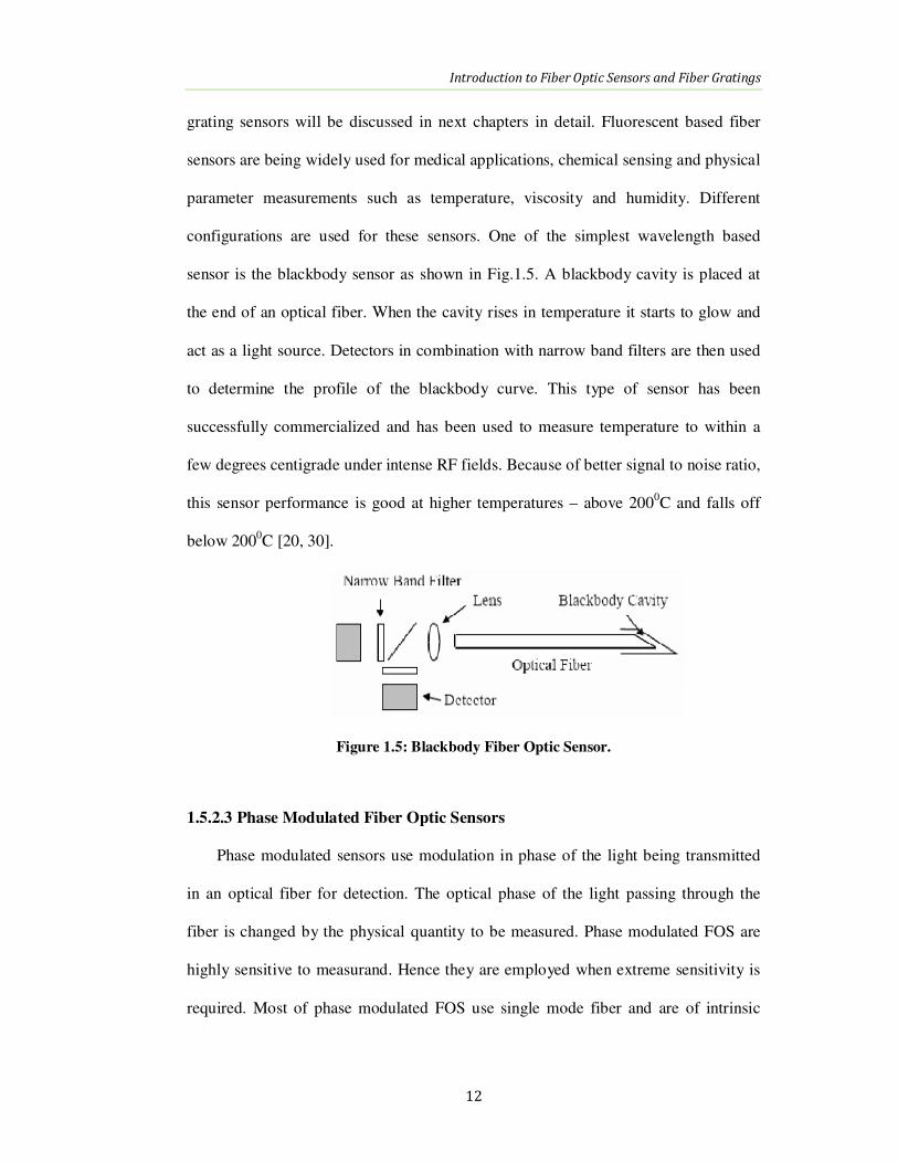
Introduction to Fiber Optic Sensors and Fiber Gratings
12
grating sensors will be discussed in next chapters in detail. Fluorescent based fiber
sensors are being widely used for medical applications, chemical sensing and physical
parameter measurements such as temperature, viscosity and humidity. Different
configurations are used for these sensors. One of the simplest wavelength based
sensor is the blackbody sensor as shown in Fig.1.5. A blackbody cavity is placed at
the end of an optical fiber. When the cavity rises in temperature it starts to glow and
act as a light source. Detectors in combination with narrow band filters are then used
to determine the profile of the blackbody curve. This type of sensor has been
successfully commercialized and has been used to measure temperature to within a
few degrees centigrade under intense RF fields. Because of better signal to noise ratio,
this sensor performance is good at higher temperatures – above 2000C and falls off
below 2000C [20, 30].
Figure 1.5: Blackbody Fiber Optic Sensor.
1.5.2.3 Phase Modulated Fiber Optic Sensors
Phase modulated sensors use modulation in phase of the light being transmitted
in an optical fiber for detection. The optical phase of the light passing through the
fiber is changed by the physical quantity to be measured. Phase modulated FOS are
highly sensitive to measurand. Hence they are employed when extreme sensitivity is
required. Most of phase modulated FOS use single mode fiber and are of intrinsic
Introduction to Fiber Optic Sensors and Fiber Gratings
13
type. The phase angle (ф) for lightwave traveling in the fiber of length L is defined as
[23]
ф =2πn L/ λ (1.1)
where ‘n’ is refractive index of the core and λ is the wavelength of light. A change in
length or refractive index under the influence of external physical parameter will
cause a phase change as defined by the equation
∆ ф =2π/ λ (n ∆L +∆n L) (1.2)
The expression n∆L+∆nL, is called optical path difference (OPD). The optical
intensity at the output of a interferometer is function of OPD. Very small change in
length produces large phase difference. Similarly, very small changes of refractive
index at longer sections of fiber produce large phase differences. When phase shift is
integral multiple of wavelength, lights from the two arms of the interferometer are in
phase providing constructive interference and maximum intensity at the output. If the
phase shift is integral multiple of half of the wavelength, lights from the two arms of
the interferometer are out of phase providing destructive interference and minimum
intensity [23].
In phase modulated sensors, this sensitive phase change of the light is encashed
to design sensor. But the difficulty is optical phase change cannot be directly detected
(optical waves have frequencies in the range of few hundred THz). The optical phase
change of the light is detected by comparing the phase with reference fiber which is
identical to measuring fiber but unperturbed by the measurand. In order to detect
phase difference, it is necessary to convert phase difference to optical intensity change
which can be measured by a detector. This is achieved by combining two optical
signals – one from sensing fiber and other from reference fiber. In an interferometer,
the light is split into two beams, where one beam is exposed to the sensing
Introduction to Fiber Optic Sensors and Fiber Gratings
14
environment and undergoes a phase shift. The other is isolated from the sensing
environment, which is used as a reference. The whole system is called interferometer.
This phase modulation is then detected interferometerically, by comparing the phase
of the light in the signal fiber to that in a reference fiber. Once the beams are
recombined, they interfere with each other. There are four most commonly used
interferometric configurations. They are - Michelson, Mach-Zehnder, Fabry-Perot and
Sagnac interferometers [22, 23, 32-35].
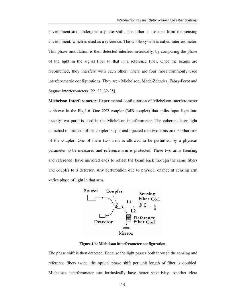
Michelson Interferometer: Experimental configuration of Michelson interferometer
is shown in the Fig.1.6. One 2X2 coupler (3dB coupler) that splits input light into
exactly two parts is used in the Michelson interferometer. The coherent laser light
launched in one arm of the coupler is split and injected into two arms on the other side
of the coupler. One of these two arms is allowed to be perturbed by a physical
parameter to be measured and reference arm is protected. These two arms (sensing
and reference) have mirrored ends to reflect the beam back through the same fibers
and coupler to a detector. Any perturbation due to physical change at sensing arm
varies phase of light in that arm.
Figure.1.6: Michelson interferometer configuration.
The phase shift is then detected. Because the light passes both through the sensing and
reference fibers twice, the optical phase shift per unit length of fiber is doubled.
Michelson interferometer can intrinsically have better sensitivity. Another clear
Introduction to Fiber Optic Sensors and Fiber Gratings
15
advantage of the Michelson interferometer is that the sensor can be designed with a
single coupler between the source-detector module. However, good-quality reflection
mirrors are required. The disadvantage of Michelson interferometer is that the coupler
feeds light into both the detector and laser. Feedback into the laser is source of noise,
especially in high performance systems [23].
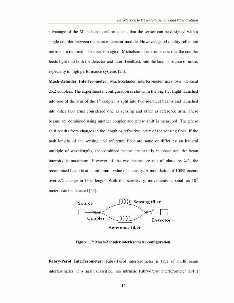
Mach-Zehnder Interferometer: Mach-Zehnder interferometer uses two identical
2X2 couplers. The experimental configuration is shown in the Fig.1.7. Light launched
into one of the arm of the 1st coupler is split into two identical beams and launched
into other two arms considered one as sensing and other as reference arm. These
beams are combined using another coupler and phase shift is measured. The phase
shift results from changes in the length or refractive index of the sensing fiber. If the
path lengths of the sensing and reference fiber are same or differ by an integral
multiple of wavelengths, the combined beams are exactly in phase and the beam
intensity is maximum. However, if the two beams are out of phase by λ/2, the
recombined beam is at its minimum value of intensity. A modulation of 100% occurs
over λ/2 change in fiber length. With this sensitivity, movements as small as 10-3
meters can be detected [23].
Figure 1.7: Mach-Zehnder interferometer configuration.
Fabry-Perot Interferometer: Fabry-Perot interferometer is type of multi beam
interferometer. It is again classified into intrinsic Fabry-Perot interferometer (IFPI)

Introduction to Fiber Optic Sensors and Fiber Gratings
16
and extrinsic Fabry-Perot interferometer (EFPI). The experimental configuration of
IFPI shown in the Fig. 1.8. It consists of two partial reflecting fiber mirrors. The
injected coherent beam is partially reflected back and partially transmitted into
interferometer. At second partial reflecting mirror, again the beam is partially
reflected and partially transmitted. In this type of interferometers, the light bounces
back and forth many times in the cavity, increasing the phase delay many times. This
transmitted light is detected through the detector at the other end. Successive
reflection sequences will reduce the detection beam. The multiple passage of light
along the fiber magnifies the phase difference resulting into highly sensitive sensor
[23, 36].
Figure 1.8: Fabry-Perot Interferometer configuration.
Fiber Optic Gyroscopes: The principle of fiber optic gyroscope is based on Sagnac
interferometry. Hence, they are also called as Sagnac interferometers. Gyroscopes are
principally used to measure rotation and are replacement for ring laser gyros and
mechanical gyros. Fiber optic gyroscopes are also used to measure time varying
effects such as angular velocity, acoustics, vibrations and slowly varying strain. Fiber
optic gyroscopes are most developed FOS. Several manufacturers worldwide are
producing them in large quantities to support automobile navigation systems, pointing
Source
Partial reflecting
mirrors
Optical fiber
Detector

Introduction to Fiber Optic Sensors and Fiber Gratings
17
and tracking of satellite antennas, inertial measurement systems for commuter aircraft
and missiles and as the backup guidance system for the Boeing 777. [20, 23, 26].
Figure 1.9: Configuration of Fiber optic gyroscope.
The basic configuration of fiber optic gyroscope is shown in Fig. 1.9. The fiber
optic gyroscope consists of loop of fiber. Light from the laser is split into two beams
and launched simultaneously into both end of the fiber loop. Both beams travel in
counter propagating directions around the loop of fiber and recombined to analyze at
a detector. In non-rotating loop, clockwise and anticlock wise beams arrive at same
time in phase and form constructive interference. If the loop is rotated in clockwise
direction, the entire coil is displaced slightly increasing the time it takes light to
traverse the fiber optic coil. Thus, the clockwise propagating light beam has to go
through a slightly longer optical pathlength than the counter-clockwise beam, which is
moving in a direction opposite to the motion of the fiber coil. Two beams reach the
detector at different times and phase difference is introduced. These differences in
arrival time and phase difference are directly proportional to the rotation rate and can
be conveniently measured as phase differences with great sensitivity and accuracy
[37-39]. Fiber optic gyroscopes are used in two configurations - open loop fiber optic
gyros and closed loop fiber optic gyros.
1.5.2.4 Polarization Modulated Fiber Optic Sensors
Standard single mode fibers transmit light without regards to polarization. But

Introduction to Fiber Optic Sensors and Fiber Gratings
18
some special fibers known as polarization mainlined fibers maintain input
polarization or transmit only one polarization state. The refractive index of a fiber
changes when fiber undergoes stress or strain depending on the direction. The
refractive index undergoing change due to stress or strain is called induced refractive
index. Because of induced refractive index, there is an induced phase difference
between different polarization directions. This phenomenon is called photoelastic
effect. The induced refractive index changes with the direction of applied stress or
strain. Thus, there is an induced phase difference between different polarization
directions. Therefore, by detecting the change in the output polarization state, the
external perturbation can be sensed. Fig. 1.10 shows the optical setup for the
polarization based fiber optic sensor. It is formed by polarizing the light from a source
via a polarizer. The polarized light is launched into polarization maintained fiber. This
section of fiber is served as sensing fiber. Under external perturbation such as stress
or strain, the phase difference between two polarization states is changed. Then, the
output polarization state is changed according to the perturbation. Hence, by
analyzing the output polarization state at the exit end of the fiber, the external
perturbation can be detected [20].
Figure 1.10: Polarization based sensor.

Introduction to Fiber Optic Sensors and Fiber Gratings
19
1.6 Fiber Gratings
Even though the improvements in optical fiber manufacturing and advancements
in the field were reality in late 1970’s; integrating optical components such as mirrors,
wavelength filters and partial reflectors to optical fibers for various applications was a
challenging job. However, all these hurdles were cleared with the discovery of fiber
gratings [40] and further refinement of fiber gating inscription method externally, that
was demonstrated by Meltz G., et. al. [41]. Fiber gratings were discovered by Hill et.
al. in 1978 [40] where the team successfully altered the core refractive index of a
single-mode optical fiber by optical absorption of UV light.
The change in core refractive index can be explained in terms of photosensitivity
of optical fibers, that allows the fabrication of phase structures in the core of fibers.
These phase structures or phase gratings are obtained by permanently changing the
refractive index in a periodic pattern along the core of the fiber. The grating period
and length together with the strength of the modulation of the refractive index
determine whether the grating has a high or low reflectivity over a wide or narrow
range of wavelengths. Therefore, these parameters determine whether the grating acts
as a wavelength division multiplexer in telecommunications, a narrow-band high-
reflectance mirror in laser or sensor applications or a wavelength-selective filter
removing unwanted laser frequencies [42].
Fiber grating is periodic perturbation along the optical path. Fiber grating is an
optical device with periodic perturbation along short section of the optical fiber core.
This perturbation in the fiber may be either in the form of refractive index, thickness
or density of glass. Most of the fiber gratings have periodic refractive index
modulation in the core that poses perturbation to the optical path. When light
propagates through periodically alternating regions of higher and lower refractive

Introduction to Fiber Optic Sensors and Fiber Gratings
20
index, it is partially reflected and partially refracted at each interface between those
regions. This periodic perturbation in the optical path directs coupling of power from
one mode to another and pitch of the perturbation selects coupling modes. [43, 44].
Fiber grating technology is widely applicable in optical communication systems and
sensing field.
Fiber grating acts as common diffraction grating of period Λ. A light wave incident
on the grating at an angle θ1 is diffracted out with an angle θ2 (Fig. 1.11). The grating
equation is given as [45],
Λ
+=λ
θθ mnn 12 sinsin (1.3)
‘m’ is diffraction order. Now considering that incident and diffracted rays
correspond to bounded modes of optical fiber, the propagation constant β can be
defined as
effnλ
πβ
2= (1.4)
with neff = nco sinθ, where neff represents effective refractive index of the mode and nco
represents refractive index of the core [46].
Figure 1.11: Diffraction by grating.
Now Eq. 1.3 can be written as
Λ
−=π
ββ2
12 (1.5)

Introduction to Fiber Optic Sensors and Fiber Gratings
21
From this equation one can predict for which grating period the coupling occurs
between two modes of propagation constant β1 and β2 at the wavelength λ.
In uniform gratings, grating planes are perpendicular to the fiber axis and are of a
constant period. These grating periods are considered as fundamental building blocks
of fiber gratings. In general fiber gratings consists of the periodic refractive index
modulation in the optical fiber core. The pitch is called period of the grating (Λ) as
shown in Fig.1.12.
Figure 1.12: Fiber grating.
Fiber gratings are broadly divided into two types based on the grating period and
light coupling scheme.
– fiber Bragg gratings also called short period gratings or reflecting gratings
– long period gratings also called transmission gratings
The relative grating period of both types of fiber gratings can be realized by observing
Fig.1.13 where there is large difference in grating period.
Figure 1.13: (a) Fiber Bragg grating (b) Long period grating.
Introduction to Fiber Optic Sensors and Fiber Gratings
22
1.6.1 Fiber Bragg Grating (FBG)
Fiber Bragg gratings consists of periodic modulation of refractive index in the
core of single mode fiber with grating period less than 100µm, practically submicron
period. FBGs act as narrow band reflection filters. FBG couples forward coupling
core mode to backward coupling core modes those scattered by grating planes,
reflecting back a small band of source spectrum [42, 47]. Reflected spectrum can be
observed in optical spectrum analyzer using 2x2 coupler or circulators. In transmitted
spectrum of FBG, a narrow band will be missing as it is reflected back. Input and
reflected spectra of typical FBG are shown in Fig.1.14. Advantages of FBGs is that-
in FBGs information is encoded in absolute parameter i.e. wavelength, they can act as
point sources, any number of FBGs can be multiplexed in single line. More
discussion on FBG will be continued in next the chapter.
Figure 1.14: FBG action.
1.6.2 Long Period Grating (LPG)
Long period gratings have grating period ranging between 100µm to 1mm. LPGs
promotes coupling between forward coupling core mode and co propagating cladding
modes. Hence, the transmitted spectrum of LPG consists of series of attenuation dips
centered at discrete wavelengths. Each attenuation dip corresponds to each cladding
mode [48]. These modes decay rapidly as they propagate along the fiber axis because

Introduction to Fiber Optic Sensors and Fiber Gratings
23
of scattering. LPG acts as band rejection filter [49]. For practical applications,
transmitted spectrum of LPG is observed. Typical input and transmitted spectrum is
shown in the Fig. 1.15.
Figure 1.15: Input and transmitted spectrum of LPG.
1.7 Lightwave Applications of FBG
An enthusiastic scenario where FBG’s are liberally applied to enhance the
lightwave network all the way from the central office to the subscriber’s premise.
Despite competitive technologies, many of these grating applications have matured,
others are nearing commercialization and, as lightwave systems evolve to optical
networks and fiber moves toward the home, the number of uses will increase. Some
light wave applications of FBG are briefly discussed below.
Laser Stabilization: Fiber Bragg grating reflectors are used as feedback mirrors in
wavelength-stabilized semiconductor lasers. Wavelength-stabilized 980nm pump
lasers [50, 51] for erbium-doped fiber amplifiers are commonly deployed today,
benefiting both pump laser yield and amplifier reliability. Grating stabilization of
1480nm pump lasers has also attracted attention [51]. Stabilization is achieved using
weak, narrow-band FBG reflectors in the fiber pigtail to couple light back into a
Fabry–Perot pump laser, creating an external laser cavity. Grating reflectivities of 1–
10% are chosen to achieve robust stabilization and maximize the laser output. Having

Introduction to Fiber Optic Sensors and Fiber Gratings
24
a narrow reflection bandwidth of 0.2–3nm allows the pump wavelength to be
accurately placed for optimum pumping of the fiber amplifier. This is particularly
important with 980 nm pumping as the erbium absorption bandwidth is only 7–10 nm
[52]; pump wavelength fluctuations from temperature, injection current and aging are
then significant risks to optimum amplifier performance. The use of a single FBG
reflector to simultaneously stabilize three pump lasers for use in multistage optical
amplifiers has been demonstrated. This reduces the number of gratings and provides
pump redundancy to increase the amplifier’s reliability [53, 54].
Fiber Lasers: Fiber lasers can be constructed using FBGs as wavelength-selective
resonator mirrors and erbium-doped fiber as the gain medium. These fiber lasers are
optically pumped, often directly without the use of pump wavelength division
multiplexing (WDM) couplers. Narrow line width fiber lasers suitable as externally-
modulated continuous wave sources have been demonstrated in gigabit/s transmission
experiments [55] and short distributed-feedback fiber lasers having Er–Yb-doped gain
sections have also exhibited robust single-frequency operation [56]. Low-cost
configurations have been proposed using 650 nm lasers to pump the erbium doped
gain region [53]. The output behavior is described by a simple above-threshold, two-
mirror model of the erbium fiber laser derived from rate equations. The laser
threshold and slope efficiency are easily calculated, whether pumped at 650, 980 or
1480 nm wavelength [57].
Reflectors in Fiber Amplifiers: Numerous fiber amplifier configurations have been
proposed to utilize reflectors or filters to enhance performance. Reflecting only the
pump light may increase the amplifier saturated output power in those cases of
amplifiers having marginal pump power. FBG’s can be used as efficient wavelength-
selective reflectors that discriminate between pump and signal light. A simple
Introduction to Fiber Optic Sensors and Fiber Gratings
25
analytical of the erbium-doped fiber amplifier [58] can be adapted to the idealized
case of negligible amplified spontaneous emission and unity reflectance of the FBG
reflector. Typically, reflecting the signal doubles the small-signal gain while
reflecting the pump may yield a 1–3dB improvement in small-signal gain. Pump
reflectors have been used to enhance performance of remotely pumped amplifiers in
repeaterless systems. Span lengths were extended by placing remote sections of
erbium doped fiber and pumping them at 1485 nm with light generated from high-
power lasers located at a terminal station. Demonstrations of greater than 500 km
repeaterless transmission at 2.5 Gb/s [59-60] and 352 km of 8 10 Gb/s [61] have been
reported. In the 352 km transmission experiment, a preamplifier 123 km from the
terminal station was remotely pumped with light from a 1.3-W source and residual
pump light was reflected back into the amplifier with a FBG reflector [54].
Raman-Shifted Lasers and Raman Amplifiers: Raman-shifted lasers and Raman
amplifiers enable efficient conversion of short-wavelength light into longer
wavelengths suitable for long-distance fiber transmission. Raman gain is obtained
through energy transfer from the pump light to the laser output or amplified signal as
mediated by molecular vibrations in the silica fiber [62]. A high-power Raman-shifted
pump laser was used to generate the 1485nm light used in the repeaterless
experiments mentioned in the previous section. In those experiments FBG resonator
mirrors enhanced the Raman amplification to convert 6 W of 1117nm light from a
diode pumped Yb3+
cladding-pumped laser into more than 1.5W of 1485 nm. The
1117nm light was down converted through five stages of Raman gain. Having so
many gratings and conversion stages requires that the grating reflectors exhibit low
insertion loss (0.2dB) and low fiber loss for the Raman shifting process to be efficient.

Introduction to Fiber Optic Sensors and Fiber Gratings
26
Dispersion Compensators: Chromatic dispersion in transmission fiber can cause
significant distortion of optical pulses, leading to system penalties. Upgrading existing
lightwave systems to 10Gb/s channels usually requires dispersion compensators often
using long lengths of dispersion-compensating fiber [63]. In the absence of optical
nonlinearities, compensation is achieved by passing the distorted signal through a
device whose dispersion is equal to that of the transmission fiber and of opposite sign.
This compensating all-pass filter must also have sufficient optical bandwidth to accept
the signal spectrum. The FBG is one such proposed filter [64]. In an idealized model,
chirp in FBG dispersion compensators should be close to linear, resulting in a
differential delay of reflected light. Disregarding optical nonlinearities and higher-
order dispersion, the chirp is selected so that grating dispersion upon reflection
cancels that of the fiber. The grating must also be long enough to ensure that the
entire signal spectrum is accommodated.
Gain Equalizers: The useful optical bandwidth of amplified lightwave systems is
limited because of gain-narrowing through concatenated optical amplifiers. Erbium-
doped silica fiber amplifiers in particular show gain peaking at 1530 and 1560nm and
the useful gain bandwidth may be reduced to less than 10nm. Pre-emphasis of the
WDM channels at the transmitter increases the available bandwidth by equalizing the
signal-to noise ratio of the received WDM channels, but is only suited for point-to-
point systems [65]. The loss spectrum of the gain-equalizing filter must match the
erbium-gain spectrum at the nominal operating condition of the amplifier. Placing a
gain-equalizing filter inside the optical amplifier flattens the gain-spectrum and with
appropriate design, may have minimal effect on the amplifier noise figure or saturated
output power. A blazed Bragg grating has been used as a gain equalizing element, but
has not led to widespread use [66].

Introduction to Fiber Optic Sensors and Fiber Gratings
27
1.8 Lightwave Applications of LPG
Long period grating which acts as wavelength dependent loss elements has many
applications in both communication and sensors. Even though, LPG applications in
various fields are under research, lot of R&D work is under the progress. Researchers
demonstrated many applications of LPG. Following are some of LPG applications in
lightwave networks already demonstrated.
Optical filters: An LPG band pass filter has been demonstrated by darkening the
fiber core in the middle section of an LPG with a focused UV beam [67] or by
insertion of a section of a hollow-core fiber between two identical LPGs [68].
Introducing π-phase shifts along an LPG also results in special band pass filters [69],
which have found applications in actively mode-locked fiber ring lasers. LPGs can
also form multi-port couplers. It has been demonstrated both theoretically and
experimentally that the light energy coupled to the cladding mode can be collected by
using two parallel LPGs [70-73]. The transmission spectra from the two parallel
gratings are complementary to each other, one showing band rejection characteristics
and the other showing band pass characteristics. The structure of two parallel LPGs
thus operates as an all-fiber broadband add/drop multiplexer and has potential
applications in WDM systems. Recently, a broad-band optical coupler based on three
parallel identical LPGs has been demonstrated [74]. A total power transfer efficiency
of 85% at the resonance wavelength has been achieved. Other implementations
include placing a tapered fiber in parallel to an LPG [75] and writing an LPG in a
two-core fiber with slightly different cores [76]. The structure of two cascaded LPGs
has been demonstrated as a multi-channel filter for multi wavelength signal
generation in WDM systems [77]. The transmission spectrum of the filter has a

Introduction to Fiber Optic Sensors and Fiber Gratings
28
sinusoidal fringe pattern with an envelope governed by the shape of the rejection band
of the individual grating and the channel spacing can be controlled by changing the
physical separation of the two gratings [78]. A technique of generating high-
repetition-rate pulses based on cascaded LPGs has also been demonstrated [79]. When
an LPG is written in a birefringent fiber, two resonance dips appear in the
transmission spectrum, which correspond respectively to the two principal
polarizations of the fiber. Such a grating has been used to realize a wavelength-
selective fiber polarizer [80]. An extinction ratio >30dB and an insertion loss < 0.5dB
have been achieved. LPG polarizers have also been implemented with few-mode
fibers [81]. Using the polarization-dependent spectrum of an LPG, a wavelength-
switchable erbium-doped fiber ring laser has been demonstrated, where dual-
wavelength operation is accomplished by rotating the polarization plane of the fiber
laser cavity [82].
Gain flatteners for optical amplifiers: LPG filters can be considered as wavelength-
selective attenuators and therefore used as gain flatteners for erbium-doped fiber
amplifiers (EDFAs) [83, 84]. By careful control of the filter spectrum and fiber
length, the EDFA gain has been flattened to within 1dB over 40nm while producing a
noise figure below 4.0dB and an output power of nearly +15dBm [84]. Another
method of achieving broad-band gain flattening is to use a phase shifted LPG [85]. To
flatten a gain spectrum that contains several peaks, a compact module based on using
different cladding modes of a number of concatenating LPGs has been proposed [86].
More recently, an EDFA gain spectrum flattened to within 0.35dB over 30nm has
been realized by using an optimized design of step changed LPGs [87]. Other gain-
flattening schemes include etching [88] and UV trimming [89] of LPGs. Dynamic
Introduction to Fiber Optic Sensors and Fiber Gratings
29
gain flattening has been demonstrated with bending of two cascaded gratings [90] or
twisting of a grating [91, 92].
Fiber coupling: Fiber-to-fiber coupling via the cladding mode of the fiber can relax
the alignment tolerances substantially [93, 94]. A lens-free fiber-to-fiber connector
that has a long working distance and a wide alignment tolerance has been
implemented by using two matched LPGs written in a double-cladding fiber [95].
Lateral alignment tolerances of ~450µm and ~3mm for coupling losses less than 1dB
and 3dB respectively have been achieved. Laser-to-fiber coupling based on an LPG
and a lens has also been demonstrated. A working distance longer than 100µm and a
lateral tolerance of 2.5µm have been obtained [94]. Fiber-to-waveguide coupling has
also been demonstrated with a CO2-laser-induced LPG. [95, 96].
Dispersion compensation: LPGs in dispersion-tailored few-mode fibers have been
employed in dispersion compensation. Higher-order mode (HOM) dispersion
compensation using the LP02 mode can offer dispersion-slope matching to practically
any transmission fibers [97]. An HOM fiber having a propagation loss of 0.44dB/km
and a dispersion coefficient of −210ps/nm/km has been fabricated [98]. Using the
HOM dispersion-compensation scheme, a 40Gb/s hybrid Raman/erbium-amplified
system with a transmission distance of 1700km has been demonstrated [99]. A
tunable dispersion compensator that utilizes an HOM fiber and switchable LPGs has
also been made, which provides a dispersion tuning range of 435ps/nm over a
bandwidth of 30nm [100].
Introduction to Fiber Optic Sensors and Fiber Gratings
30
1.9 Potable Water
Water is most fundamental building block of life. Most of us are fortunate to be
living in a place where water is easily available. Most of the earth surface is covered
with water, there is much more water than there is land. About 70% of the earth's
surface is covered with water. Water also exists in the air as vapour and in aquifers in
the soil, as groundwater. Oceans store most of the earth's water, this is apparently
97% of the total amount of water on earth, 2% of which is frozen. Of all the water on
earth only 2.59% is freshwater. Of this, about 2% is trapped in ice caps and glaciers.
The rest of the freshwater is either groundwater (0.592%) or readily accessible water
in lakes, streams, rivers, etc. (0.014%). From the above statistics, one can conclude
that less than 1% of water on earth can be used as drinking water. This includes both
surface and ground water [101, 102].
Over large parts of the world, humans have inadequate access to potable water
and use sources contaminated with disease vectors, pathogens or unacceptable levels
of toxins or suspended solids. Drinking or using such water in food preparation leads
to widespread acute and chronic illnesses and is a major cause of death and misery in
many countries. Reduction of waterborne diseases is a major public health goal in
developing countries.
With increasing world population and run for the high profile life, it is becoming
difficult to supply safe drinking water. Industries are growing to supply the demands
of population which is also the reason for the growing water difficulty. Industries
demand more water and pollution will increase if the industrial effluents are not
managed properly. Other factors such as fertilizer runoff and leaking from septic
tanks can further contaminate water. Just because one has water source (lake, river,
well or bore well) that yields plenty of water doesn't mean you can go ahead and just

Introduction to Fiber Optic Sensors and Fiber Gratings
31
take a drink. Because water is such an excellent solvent that it can contain lots of
dissolved chemicals. Since, ground water moves through rocks and subsurface soil, it
has a lot of opportunity to dissolve substances as it moves. For that reason, ground
water will often have more dissolved substances than surface water. Even though the
ground has an excellent mechanism for filtering out matter such as leaves, soil, bugs,
dissolved chemicals and gases can still occur in large enough concentrations in
ground water to cause problems. As ground water flows through sediments, metals
such as iron, manganese, potassium, calcium, manganese, lead, cadmium, mercury,
organic compounds etc are dissolved and may later be found in high concentrations in
the water. If water is badly polluted (like raw sewage) it might be obvious from its
appearance or odor. It might be colored or turbid (cloudy) or have solids, oil or foam
floating on it. Even though water appears clean, clear and odor less it may not be fit to
drink. Many harmful and beneficial materials in water are invisible and odorless.
Higher concentration of these dissolved chemicals in water may cause serious health
problems in human by prolonged intake. A number of chemical contaminants have
been shown to cause adverse health effects in humans as a consequence of prolonged
exposure through drinking-water. In water, many radicals such as iron, manganese,
copper, cadmium, mercury, arsenic, lead, zinc, cyanides, fluorides etc are present in
ppm / ppb level. Slight increase in the concentration of these chemicals in water may
cause significant problems; even crises can occur on prolonged use of such water.
Many research and analysis were taken up in the past to recommend the
minimum level of these dissolved chemicals in the drinkable water and these
recommendations are known as standards of drinking water or guidelines for drinking
water. Every country has its own drinking water standards based on geographical
condition. World Health Organization (WHO) is universal body that regularly
Introduction to Fiber Optic Sensors and Fiber Gratings
32
releases guidelines for drinking water. The WHO Guidelines for Drinking-water
Quality (GDWQ) provide a point of reference for drinking water quality regulations
and standards all over the world.
Hence, regular monitoring of the water quality- level of dissolved chemicals
present in the water is very important. There are many methods of analysis such as
colorimetric, gravimetric, electrochemical, chromatography, mass spectrometry, etc.
But to determine metal radicals present in very low concentrations (ppm level),
specialized equipments are required such as atomic absorption spectrometer (AAS),
inductively coupled plasma (ICP) spectrometer, flow injection method. These all
instruments are laboratory based (not portable), expensive and require special
technical person to handle the instrument. In AAS every elemental analysis requires
respective light source (E.g. Iron source for Fe analysis). ICP spectrometer
experiences lot of interference of other elements while analyzing particular one [103].
Flow injection method requires preprocessing of a test sample. To avoid all these
methods, in the present work we present very simple, low cost method based on fiber
grating technology. Here, we present highly sensitive fiber grating sensor to
determine the concentration of manganese and nitrate present in water at ppm level.
Our fiber grating sensors are sensitive, robust and reliable. Results obtained by grating
sensors are confirmed by AAS and ICP methods. Later sensitivity of the sensor is
enhanced by coating sensor region with gold nanoparticles synthesized in the
laboratory.
1.10 Optical Fibers in Nuclear Environment
Since optical fibers and optical fiber components have excellent features such as
low-loss large information capacity, compactness, low insertion loss and little
Introduction to Fiber Optic Sensors and Fiber Gratings
33
influence by electromagnetic induction compared with conventional copper cable
systems, those have been applied to not only in public telecommunication, but also
space applications [104], in nuclear industry [105] and in high energy physics
experiments [106]. Hence, it has become essential to investigate the influence of
ionizing radiation on the characteristics of optical fibers and many fiber-optic
components. Radiation effects in bulk optical glasses and in optical fibers have been
extensively studied in the last decades. In bulk silica glass, different effects have been
seen such as radiation-induced attenuation, luminescence and refractive index changes
[107-111]. Transmission loss is considered to be the most affected parameter of the
optical fiber. Radiation induced changes in transmission characteristics of optical
fibers depend upon type of radiation, intensity (flux), rate of flux, total exposure,
optical fiber composition, wavelength of transmission etc. Radiation resistivity of
various types of optical fibers was therefore noted. Numerous investigations about the
resistivity and sensitivity of optical fiber are being undertaken all over the world
[112]. We studied the optical properties of plastic optical fiber and silica fiber under
nuclear radiation of gamma radiation emitted by Amerisium-241 and FBG
characteristics under radiation emitted by Na22
and Tl204
.

Introduction to Fiber Optic Sensors and Fiber Gratings
34
References
1. K. O. Kao and G. A. Hockham, "Dielectric-fibre surface waveguides for
optical frequencies," Proc. IEE 113 (7), pp.1151–1158 (1966).
2. John M. Senior “Optical Fiber Communications Principles and Practices,”
Princeton Hall Press (1992).
3. “Two revolutionary optical technologies” Compiled by the Class of Physics of
the Royal Swedish Academy of Sciences, A scientific Background on Nobel
Prize in Physics 2009.
4. J. H. Cole, R. L. Johnson and P. B. Bhuta, “Fiber optic detection of sound,” J.
Acoustic Society of America, 62, pp.1136-1138, (1977).
5. J. A. Bucaro and T. R. Hickman, “Measurement of sensitivity of optical fibers
for acoustic detection,” Applied Optics, 18, pp. 938-940, (1979).
6. N. Lagakos, E. U. Schnaus, J. H. Cole, J. Jarzynski and J. A. Bucaro,
“Optimizing fiber coatings for interferometric acoustic sensors,’’ IEEE J.
Quantum Electron., 21, pp. 683-689, (2013).
7. B. Budiansky, D. C. Drucker, G. S. Kino and J. R. Rice, “The pressure
sensitivity of a clad optical fiber,” Applied Optics, 18, pp. 4085-4088, (1979).
8. G. B. Hocker, “Fiber optic sensing of pressure and temperature,” Applied
Optics, 18, pp. 1445-1448, (1979).
9. N. Lagakos and J. A. Bucaro, “Pressure desensitization of optical fibers,”
Applied Optics, 20, pp. 2716-2720, (1981).
10. A. Yariv and H. Winsor, “Proposal for detection of magnetostrictive
perturbation of optical fibers,” Optics Letters, 5, pp. 87-89, (1980).
11. A. Dandridge, A. B. Tveten, G. H. Sigel, Jr., E. J. West and T. G.Giallorenzi,
“Optical fiber magnetic field sensor,’’ Electronic Letters, 16, pp. 408-409,
(1980).
12. S. C. Rashleigh, “Magnetic field sensing with a single mode fiber,” Optics
Letters, 6, pp. 19-21,(1981).
13. A. Bergh, H. C. Leferere and H. J. Shaw, “All-single-mode fiber-optic
gyroscope,” Optics Letters, 6, pp. 198-200, (1981).
14. H. J. Arditty, M. Papuchon and C. Puech, “Fiber-optic rotation sensor:
Toward an integrated device. A review,” in Proc. CLEO I981, pp. 9-11,
(1981).

Introduction to Fiber Optic Sensors and Fiber Gratings
35
15. A. Dandridge, A. B. Tveten and T. G. Giallorenzi, “Interferometric current
sensors with optical fibers,” Electronics Letters., 17, pp. 523-524, (1981).
16. G. L. Tangonan, D. I. Persechimi, R. J. Morrison and T. A. Wysocki, “Current
sensing with metal coated multimode fibers,” Electronics Letters, 16, pp. 958,
(1980).
17. Thomas G. Giallorenzi, Joseph A. Bucaro, Anthony Dandridge, G. H. Sigel,
Jr., James H. Cole, Scott C. Rkshleigh, and Richard G. Priest, “Optical fiber
sensor technology ,” IEEE Journal Of Quantum Electronics, Qe-18, pp. 626-
665, (1982).
18. Bishnu P. Pal “Fundamental of Fiber Optics in Telecommunication and
Sensing Systems” New Age International Limited, New Delhi (2013).
19. Bahareh Gholamzadeh and Hooma Nabovati, “Fiber Optic Sensors”
Proceedings of Academy of Science Engineering and Technology, vol 32,
pp.303-313, (2008).
20. K. A. Fidanboylu and H. S. Efendioglu, “Fiber optic sensors and their
applications” 5th International Advanced Technologies Symposium (IATS’09),
Keynote May 13-15, Karabuk, Turkey, (2009).
21. B. Lee, “Review of Present Status of Optical Fiber Sensors,” Optical Fiber
Technology, 9, pp. 57-79, (2003).
22. K.T.V. Grattan and Dr. T. Sun, “Fiber optic sensor technology: an overview,”
Sensors and Actuators A, 82, pp. 40–61, (2000).
23. D. A. Krohn, “Fiber Optic Sensors Fundamentals and Applications,”
Instruments Society of America (1998).
24. S. D. Schwab and R. L. Levy, “In-service characterization of composite
matrices with an embedded fluorescence optrode sensor,” Proc. SPIE, 1170,
pp. 230, (1989).
25. K. T. V. Grattan, R. K. Selli and A. W. Palmer, “A miniature fluorescence
referenced glass absorption thermometer,” Proc. 4th Intl. Conf. Optical Fiber
Sensors, Tokyo, pp. 315, (1986).
26. Eric Udd “Overview of fiber optic sensors” Edited by Francis T. S. Yu and
Shizhuo Yin, “Fiber Optic Sensors,” Eastern Hemisphere Distribution, Marcel
Dekker, Inc. (2002).
Introduction to Fiber Optic Sensors and Fiber Gratings
36
27. W. W. Morey, G. Meltz and W. H. Glenn, “Bragg–grating temperature and
strain sensors, Proc. Optical Fiber Sensors,” Springer-Verlag, Berlin, 89, pp.
526, (1989).
28. G. A. Ball, G. Meltz and W. W. Morey, “Polarimetric heterodyning Bragg–
grating fiber laser sensor,” Optics Letters, 18, pp. 1976-1978, (1993).
29. J. R. Dunphy, G. Meltz, F. P. Lamm and W. W. Morey, “Multi-function,
distributed optical fiber sensor for composite cure and response monitoring,”
Proc. SPIE, 1370, pp.116, (1990).
30. Eric Udd, Whitten Schulz, John Seim, John Corones, H. Martin Laylor “Fiber
optic sensors for infrastructure applications,” Report submitted to Federal
Highway Administration 400 Seventh Street S.W., Washington D.C. 20590,
(1998).
31. Denis Donlagic, “Fiber optic sensor: An introduction and overview”
32. D.A. Flavin, R. Mcbride, J.D.C. Jones, “Interferometric fiber optic sensing
based on the modulation of group delay and first order dispersion: application
to strain-temperature measurand,” J. Lightwave Technology, 13, pp.1314-
1321, (1995).
33. A.M. Vengsarkar, W.C. Michie, L. Jankovic, B. Culshaw, R.O. Claus, “Fiber-
optic dual-technique sensor for simultaneous measurement of strain and
temperature,” J. Lightwave Technology, 12, pp. 170-177, (1994).
34. V. Vali and R. W. Shorthill, “Fiber ring interferometers,” Applied Optics, 15,
pp.1099, (1976).
35. C.E. Lee and H.F. Taylor “Interferometric optical fiber sensors using internal
mirrors,” Electronics Letters, 24, pp. 193-194, (1988).
36. K.A. Murphy, “Extrinsic Fabry–Perot optical fiber sensor,” in: Proc. OFS-8,
Monterey, CA, pp. 193-196, (1992).
37. Brian Culshaw and Alan Kersey, “Fiber-Optic Sensing: A Historical
Perspective,” J. Lightwave Technology, 26 (9), pp. 1064-78, (2008).
38. Ali Reza Bahrampour, Sara Tofighi, Marzieh Bathaee and Farnaz Farman,
“Optical Fiber Interferometers and Their Applications,” Interferometry –
Research and Applications in Science and Technology.
39. www.intechopen.com.

Introduction to Fiber Optic Sensors and Fiber Gratings
37
40. K. O. Hill, Y. Fujii, D. C. Johnson and B. S. Kawasaki, “Photosensitivity in
optical fibre waveguides: application to reflection filter fabrication,” Applied
Physics Letters, 32, pp. 647-649 (1978).
41. G. Meltz, W. W. Morey and W. H. Glenn, “Formation of Bragg gratings in
optical fibre by a transverse holographic method,” Optics Letters, 14 pp.823–
825, (1989).
42. Andreas Othonos, “Fiber Bragg gratings,” Review of Scientific Instruments,
68, pp. 4309-4341, (1997).
43. Ho Sze Phing, Jalil A li, Rosly Abdul Rahman and Bashir Ahmed Tahir,
“Fiber Bragg grating modeling, simulation and characteristics,” Journal of
Fundamental Sciences, 3, pp.167-175, (2007).
44. Sunita Ugale and V. Mishra, “Fiber Bragg grating modeling, characterization
and optimization with different index profiles,” International Journal of
Engineering Science and Technology, 2, pp.4463-4468, (2010).
45. Max Born and E. Wolf, “Principles of Optics,” Cambridge University Press,
7th Edition, (1999).
46. Turan Erdogan “Fiber grating spectra,” J. Lightwave Technology, 15,
pp.1277-1294, (1997).
47. Y. J. Rao, “In-fiber Bragg grating sensors,” Measurement Science &
Technology, 8, pp. 322-375, (1997).
48. S. W. James and Ralph P Tatam, “Optical fiber long period gratings sensors:
characteristics and application,” Measurement Science & Technology, 14,
R49-R61, ( 2003).
49. Ashish M. Vengsarkar, Paul J. Lemaire, Justin B. Judkins, Vikram Bhatia,
Turan Erdogan and John E. Sipe “Long period fiber gratings as band rejection
filter,” J. Lightwave Technology, 14,pp.58-65, (1996).
50. B. F. Ventrudo, G. A. Rogers, G. S. Lick, D. Hargreaves and T. N. Demayo,
“Wavelength and intensity stabilization of 980 nm diode lasers coupled to
fiber Bragg gratings,” Electronics Letters, 30(25), pp. 2147–2149, (1994).
51. A. Hamakawa, T. Kato, G. Sasaki and M. Higehara, “Wavelength stabilization
of 1.48 µm pump laser by fiber grating,” in Proc. ECOC’96, Oslo, Norway,
paper MoC.3.6., (1996).
Introduction to Fiber Optic Sensors and Fiber Gratings
38
52. W. J. Miniscalco, “Erbium-doped glasses for fiber amplifiers at 1500nm,” J.
Lightwave Technol., 9, pp. 234–250, (1991).
53. C. R. Giles, T. Erdogan and V. Mizrahi, “Reflection-induced changes in the
optical spectra of 980 nm QW lasers,” IEEE Photonics Technology Letters, 6,
pp. 903–906, (1994).
54. C. R. Giles, “Lightwave applications of fiber Bragg gratings,” J. Lightwave
Technol., 15 (8), pp 1391-1404, (1997)
55. J. L. Zyskind, J. W. Sulhoff, P. D. Magill, K. C. Reichmann, V. Mizrahi and
D. J. DiGiovanni, “Transmission at 2.5 Gbit/s over 654 km using an erbium-
doped fiber grating laser source,” Electronics Letters, 29, pp. 1105, (1993).
56. J. T. Kringlebotn, P. R. Morkel, L. Reekie, J. L. Archambault and D. N.
Payne, “Efficient diode-pumped single frequency erbium: ytterbium fiber
laser,” IEEE Photonics Technology Letters, 5, pp. 1162, (1993).
57. C. R. Giles and E. Desurvire, “Modeling erbium-doped fiber amplifiers,” J.
Lightwave Technol., 9, pp. 271–283, (1991).
58. A. A. M. Saleh, R. M. Jopson, J. D. Evankow and J. Aspell, “Modeling of gain
in erbium-doped fiber amplifiers,” IEEE Photon. Technol. Lett., 2, pp. 714-
717, (1990).
59. P. B. Hansen, L. Eskildsen, S. G. Grubb, A. M. Vengsarkar, S. K. Korotky, T.
A. Strasser, J. E. J. Alphonsus, J. J. Veselka, D. J. DiGiovanni, P. W.
Peckham, E. C. Beck, D. Truxal, W. Y. Cheung, S. G. Kosinski, D. Gaspar, P.
F. Wysocki, V. L. da Silva and J. R. Simpson, “2.488-Gb/s unrepeatered
transmission over 529 km using remotely pumped post-and pre-amplifiers,
forward error correction and dispersion compensation,” in Proc. OFC ’95, San
Diego, CA,PD-25, (1995).
60. S. Sian, O. Gautheron, M. S. Chaudhry, C. D. Stark, S. Webb, K. Guild, M.
Mesic, J. M. Dryland, J. R. Chapman, A. R. Docker, E. Brandon, T. Barbier,
P. Garabedian and P. Bousselet, “511km at 2.5 Gbit/s and 531km at 622
Mbit/s-unreapeatered transmission with remote pumped amplifiers, forward
error correction and dispersion compensation,” in Proc. OFC’95, San Diego,
CA, PD-26, (1995).
61. P. B Hansen, L. Eskildsen, S. G. Grubb, A. M. Vengsarkar, S. K. Korotky, T.
A. Strasser, J. E. J. Alphonsus, J. J. Veselka, D. J. DiGiovanni, D. W.

Introduction to Fiber Optic Sensors and Fiber Gratings
39
Peckham, D. Truxal, W. Y. Cheung, S. G. Kosinski and P. F. Wysocki,
“Unrepeatered WDM transmission experiment with 8 channels of 10 Gb/s
over 352 km,“ IEEE Photonics Technology Letters, 8, pp. 1082–1084, (1996).
62. A. R. Chraplyvy, “Limitations on lightwave communications imposed by
optical-fiber nonlinearities,” J. Lightwave Technol., 8, pp.1548–1557, (1990).
63. R. J. Nuyt, Y. K. Park and P. Gallion, “Dispersion equalization of a 10 Gb/s
repeatered transmission system using dispersion compensating fiber,” J.
Lightwave Technol., 15, pp. 31–42, (1997).
64. F. Ouellette, “Dispersion cancellation using linearly chirped Bragg grating
filters in optical waveguides,” Optics Letters, 12, pp. 847–849, (1987).
65. A. R. Chraplyvy, J. A. Nagel and R. W. Tkach, “Equalization in amplified
WDM lightwave transmission systems,” IEEE Photonics Technology Letters,
4, pp. 920–922, (1992).
66. R. Kashyap, R. Wyatt and R. J. Campbell, “Wideband gain flattened erbium
fiber ampifier using a photosensitive fiber blazed gating,” Electronics Letters,
29, pp.154–156, (1993).
67. D. S. Starodubov, V. Grubsky and J. Feinberg, “All fiber band pass filter with
adjustable transmission using cladding-mode coupling,” IEEE Photonics
Technology Letters, 10(11), pp.1590–1592, (1998).
68. S. Choi, T. J. Eom, Y. Jung, B. H. Lee, J. W. Lee and K. Oh, “Broad-band
tunable all-fiber band pass filter based on hollow optical fiber and long-period
grating pair,” IEEE Photonics Technology Letters, 7(1), pp.115–117, (2005).
69. F. Y. M. Chan and K. S. Chiang, “Analysis of apodized phase-shifted long-
period fiber gratings,” Optics Communications, 244(1-6), pp. 233-243, (2005).
70. H. Ke, K. S. Chiang and J. H. Peng, “Analysis of phase shifted long-period
fiber gratings,” IEEE Photonics Technology Letters, 10(11), pp. 1596-1598,
(1998).
71. O. Deparis, R. Kiyan, O. Pottiez and M. Blondel, “Bandpass filters based on
p-shifted long-period fiber gratings for actively mode-locked erbium fiber
lasers,” Optics Letters, 26(16), pp. 1239-1241, (2001).
72. K. S. Chiang, Y. Q. Liu, M. N. Ng and S. P. Li, “Coupling between two
parallel long-period fibre gratings,” Electronics Letters, 36(16), pp. 1408-
1409, (2000).
Introduction to Fiber Optic Sensors and Fiber Gratings
40
73. K. S. Chiang, F. Y. M. Chan and M. N. Ng, “Analysis of two parallel long-
period fiber gratings,” J. Lightwave Technol., 22(5), pp. 1358-1366, (2004).
74. Y. Liu and K. S. Chiang, “Broad-band optical coupler based on evanescent-
field coupling between three parallel long-period fiber gratings,” IEEE
Photonics Technology Letters, 18(1), pp. 229-231, (2006).
75. A. P. Luo, K. Gao, F. Liu, R. H. Qu and Z. J. Fang, “Evanescent-field
coupling based on long period grating and tapered fiber,” Optics
Communications, 240(1-3), pp. 69-73, (2004).
76. H. L. An, B. Ashton and S. Fleming, “Long-period grating- assisted optical
add-drop filter based on mismatched twin-core photosensitive-cladding fiber,”
Optics Letters, 29(4), pp. 343-345 (2004).
77. X. J. Gu, “Wavelength-division multiplexing isolation fiber filter and light
source using cascaded long-period fiber gratings,” Optics Letters, 23(7), pp.
509-510, (1998).
78. B. H. Lee and J. J. Nishii, “Dependence of fringe spacing on the grating
separation in a long-period fiber grating pair,” Applied Optics, 38(16), pp.
3450-3459, (1999).
79. T. J. Tom, S. J. Kim, C. S. Park and B. H. Lee, “Generation of high-repetition-
rate optical pulse using cascaded long-period fibre gratings,” Electronics
Letters, 40(16), pp. 981-982, (2004).
80. B. Ortega, L. Dong, W. F. Liu, J. P. Desandro, L. Reekie, S. I. Tsypina, V. N.
Bagratashvili and R. I. Laming, “High-performance optical fiber polarizers
based on long-period gratings in birefringent optical fibers,” IEEE Photonics
Technology Letters, 9(10), pp. 1370- 1372 (1997).
81. S. Ramachandran, M. Das, Z. Wang, J. Fleming and M. Yan, “High
extinction, broadband polarisers using long period fibre gratings in few-mode
fibres,” Electronics Letters, 38(22), pp. 1327-1328, (2002).
82. Y. W. Lee and B. Lee, “Wavelength-switchable Erbium doped fiber ring laser
using spectral polarization dependent loss element,” IEEE Photonics
Technology Letters, 15(6), pp. 795-797 (2003).
83. A. M. Vengsarkar, J. R. Pedrazzani, J. B. Judkins, P. J. Lemaire, N. S.
Bergano and C. R. Davidson, “Long period fiber-grating-based gain
equalizers,” Optics Letters, 21(5), pp. 336-338, (1996).

Introduction to Fiber Optic Sensors and Fiber Gratings
41
84. P. F. Wysocki, J. B. Judkins, R. P. Espindola, M. Andrejco and A. M.
Vengsarkar, “Broad-band Erbium doped fiber amplifier flattened beyond 40
nm using long period grating filter,” IEEE Photonics Technology Letters,
9(10), pp. 1343-1345, (1997).
85. J. R. Qian and H. F. Chen, “Gain flattening fiber filters using phase shifted
long period fiber gratings,” Electronics Letters, 34(11), pp. 1132-1133, (1998).
86. M. Harumoto, M. Shigehara, M. Kakui, H. Kanamori and M. Nishimura,
“Compact long-period grating module with multi-attenuation peaks,”
Electronics Letters, 36(6), pp. 512-514, (2000).
87. A. P. Zhang, X. W. Chen, Z. G. Guan, S. L. He, H. Y. Tam and W. H. Chung,
“Optimization of step-changed long-period gratings for gain-flattening of
EDFAs,” IEEE Photonics Technology Letters, 17(1), pp. 121-123, (2005).
88. C. E. Chou, N. H. Sun and W. F. Liu, “Gain flattening filter of an erbium-
doped fiber amplifier based on etching long-period gratings technology,”
Optical Engineering, 43(2), pp.342-345, (2004).
89. M. Harumoto, M. Shigehara and H. Suganuma, “Gain flattening filter using
long-period fiber gratings,” J. Lightwave Technology, 20(6), pp. 1027-1033,
(2002).
90. M. K. Pandit, K. S. Chiang, Z. Chen and S. P. Li, “Tunable long-period fiber
gratings for EDFA gain and ASE equalization,” Microwave Optical
Technology Letters, 25(3), pp. 181-184, (2000).
91. Y. J. Rao, A. Z. Hu and Y. C. Niu, “A novel dynamic LPFG gain equalizer
written in a bend-insensitive fiber,” Optics Communications, 244(1-6), pp.
137-140, (2004).
92. T. Zhu, Y. J. Rao and L. J. Wang “All fiber dynamic gain equalizer based on a
twisted long period grating written by high frequency CO2 laser pulses,”
Applied Optics, 46(3), pp 375-378 .
93. W. T. Chen and L. A. Wang, “Optical coupling between single mode fibres by
utilizing long-period fibre gratings,” Electronics Letters, 35(5), pp. 421-423,
(1999).
94. Wen-Yueh Su, Gia-Wei Chern And Lon A. Wang, “Analysis of cladding-
mode couplings for a lensed fiber integrated with a long-period fiber grating

Introduction to Fiber Optic Sensors and Fiber Gratings
42
by use of the beam-propagation method,” Applied Optics, 41(31), pp. 6576-
6584, (2002).
95. M. J. Kim, T. J. Eom, U. C. Paek and B. H. Lee, “Lens free optical fiber
connector having a long working distance assisted by matched long-period
fiber gratings,” J. Lightwave Technology, 23(2), pp. 588-596, (2005).
96. B. L. Bachim, O. O. Ogunsola and T. K. Gaylord, “Optical-fiber-to-waveguide
coupling using carbon dioxide- laser-induced long-period fiber gratings,”
Optics Letters, 30(16), pp. 2080-2082, (2005).
97. Kin Seng Chiang and Qing Liu “Long-period grating devices for application
in optical communication” Optoelectronics Research Centre and Department
of Electronic Engineering City University of Hong Kong, 83 Tat Chee
Avenue, Kowloon, Hong Kong, China.
98. S. Ghalmi, S. Ramachandran, E. Monberg, Z. Wang, M. F. Yan, F. V.
Dimarcello, W. A. Reed, P. Wisk and J. Fleming, “Low loss, all-fiber high-
order mode dispersion compensators for lumped or multi-span compensation,”
Electronics Letters, 38(24), pp. 1507–1508, (2002).
99. S. Ramachandran, G. Raybon, B. Mikkelsen, M. F. Yan, L. Cowsar and R.-J.
Essiambre, “1700km transmission at 40Gb/s with 100km amplifier-spacing
enabled by higher-order-mode dispersion-compensation,” Electronics Letters,
37(22), pp. 1352–1354, (2001).
100. S. Ramachandran, S. Ghalmi, S. Chandrasekhar, I. Ryazansky, M. Yan, F.
Dimarcello, W. Reed and P. Wisk, “Tunable dispersion compensators utilizing
higher order mode fibers,” IEEE Photonics Technology Letters, 15(5), pp.
727–729, (2003).
101. http://en.wikipedia.org/wiki/H2O
102. http://www.lenntech.com/home
103. Douglas K. Skoog, F. Jamse Holler, Timothy A. Nieman, “Principles of
Instrumental Analysis,” Harcourt Asia PTE LTD, (1998).
104. A. F. Fernandez, F. Berghmans, B. Brichard and M. Decreton, “Toward the
development of radiation-tolerant instrumentation data links for thermonuclear
fusion experiments,” IEEE Transactions on Nuclear Science, 49, pp. 2879–
2887, (2002).
Introduction to Fiber Optic Sensors and Fiber Gratings
43
105. E. Friebele, M. E. Gingerich and D. Griscom, “Survivability of optical fibers
in space,” Proc. SPIE, 1791, pp. 177–188, (1992).
106. K. Gill, R. Grabit, J. Troska and F.Vasey, “Radiation hardness qualification of
InGaAsP/InP 1310-nm lasers for the CMS tracker optical links,” IEEE Trans.
Nucl. Sci., 49, pp. 2923–2929, (2002).
107. D. Griscom, “Optical properties and structure of defects in silica glass,” J.
Ceramic Society of Japan, 99, pp. 899–916, (1991).
108. L. Skuja, “Optically active oxygen-deficiency-related centers in amorphous
silicon dioxide,” J. Non-Crystalline Solids, 239, pp. 16–48, (1998).
109. W. Primak, “The compacted states of vitreous silica,” in Studies of Radiation
Effects in Solids, G. Dienes and L. Chadderton, Eds. New York: Gordon and
Breach, 4, ( 1975).
110. E. Taylor, K. Hulick, J. Battiato, A. Sanchez, J. Winter and A. Pirich,
“Response of germania doped fiber Bragg gratings in radiation environments,”
Proc. SPIE, 3714, pp. 106–113, (1999).
111. A. Fernandez, B. Brichard, F. Berghmans and M. Décreton, “Dose-rate
dependencies in gamma-irradiated in-fiber Bragg gratings,” IEEE
Transactions on Nuclear Science, 49, pp. 2874–2878, (2002).
112. R. H. West “A local view of radiation effects in fiber optics,” J. Lightwave
Technology, 6, pp. 155-164, (1998).


![Threats to Fiber- Optic Infrastructures · lMCI targeting Verizon for brand damage [tap disclosures] ... Defending Fiber Optic InfrastructuresDefending Fiber Optic Infrastructures.](https://static.fdocuments.us/doc/165x107/5acb82e77f8b9ab10a8b583f/threats-to-fiber-optic-targeting-verizon-for-brand-damage-tap-disclosures-.jpg)