1058 Teradata Indexes How they work and when to use them …€¦ · – Capture table usage, then...

#TDPARTNERS16 Sept 11,2016 GEORGIA WORLD CONGRESS CENTER

TERADATA INDEXES: How they work and when to use them

Session ID: 0158 Sunday 2:00 PM – Room C110

Alison Torres

Solution Architect, Teradata

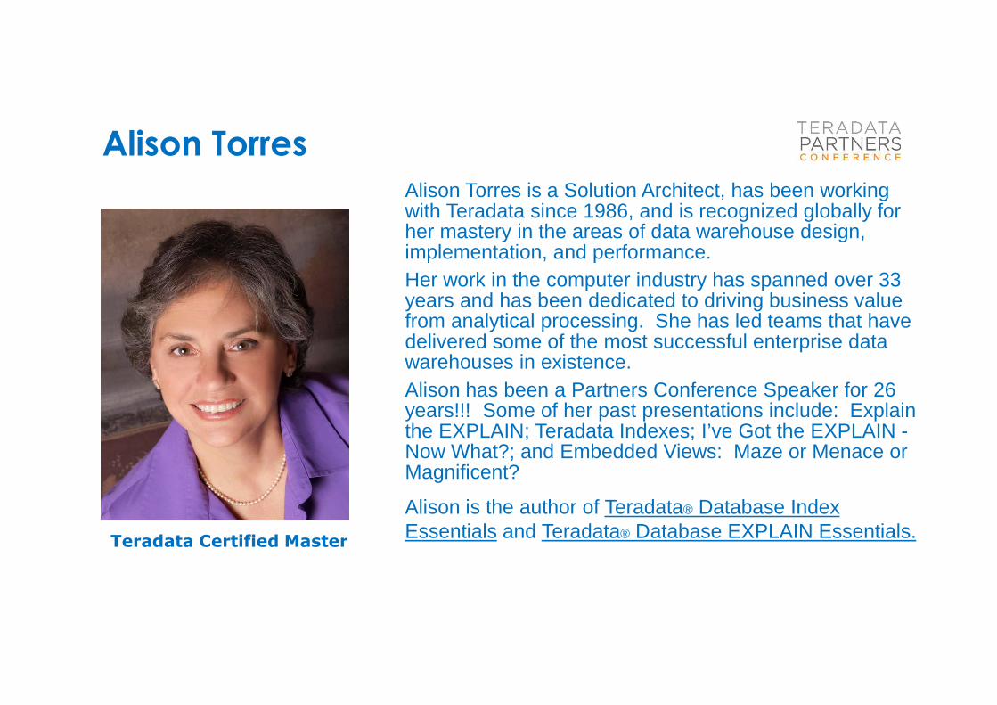
Alison Torres

Alison Torres is a Solution Architect, has been working with Teradata since 1986, and is recognized globally for her mastery in the areas of data warehouse design, implementation, and performance. Her work in the computer industry has spanned over 33 years and has been dedicated to driving business value from analytical processing. She has led teams that have delivered some of the most successful enterprise data warehouses in existence. Alison has been a Partners Conference Speaker for 26 years!!! Some of her past presentations include: Explain the EXPLAIN; Teradata Indexes; I’ve Got the EXPLAIN -Now What?; and Embedded Views: Maze or Menace or Magnificent?

Alison is the author of Teradata® Database Index Essentials and Teradata® Database EXPLAIN Essentials.

Teradata Certified Master

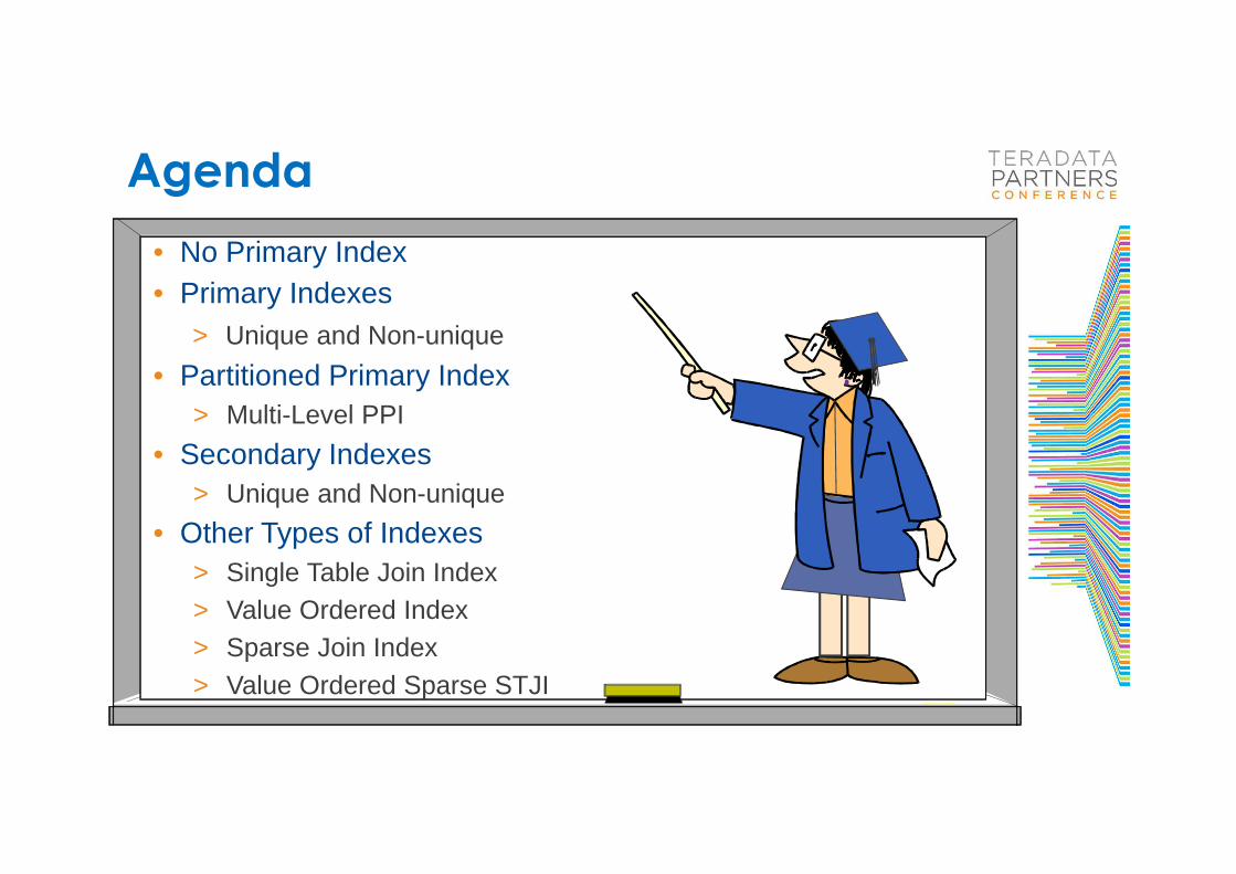
Agenda

• No Primary Index• Primary Indexes

> Unique and Non-unique

• Partitioned Primary Index> Multi-Level PPI

• Secondary Indexes> Unique and Non-unique

• Other Types of Indexes> Single Table Join Index> Value Ordered Index> Sparse Join Index> Value Ordered Sparse STJI

No Primary Index

• No Primary Index Tables

Tables without a Primary Index

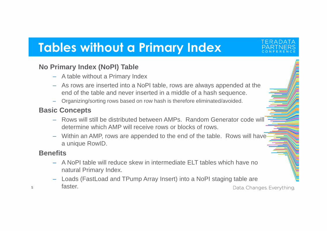
No Primary Index (NoPI) Table– A table without a Primary Index– As rows are inserted into a NoPI table, rows are always appended at the

end of the table and never inserted in a middle of a hash sequence.– Organizing/sorting rows based on row hash is therefore eliminated/avoided.

Basic Concepts – Rows will still be distributed between AMPs. Random Generator code will

determine which AMP will receive rows or blocks of rows. – Within an AMP, rows are appended to the end of the table. Rows will have

a unique RowID.

Benefits– A NoPI table will reduce skew in intermediate ELT tables which have no

natural Primary Index.– Loads (FastLoad and TPump Array Insert) into a NoPI staging table are

faster.5

When to Use No Primary Index

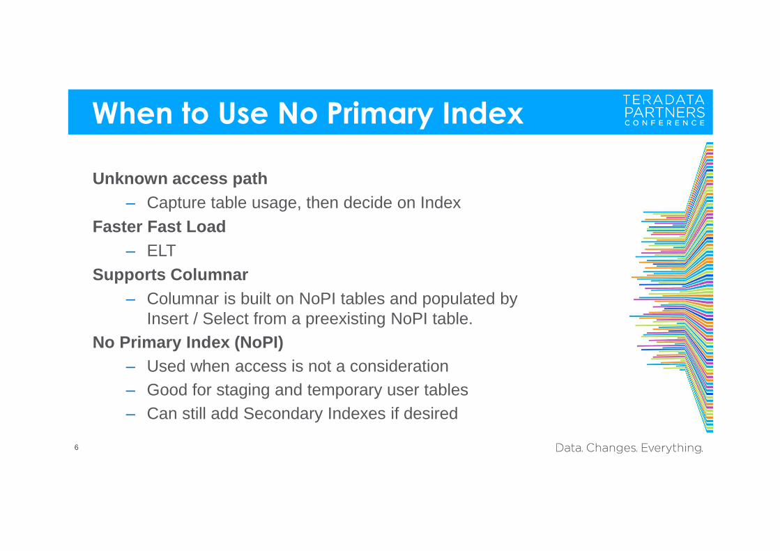
Unknown access path– Capture table usage, then decide on Index

Faster Fast Load– ELT

Supports Columnar – Columnar is built on NoPI tables and populated by

Insert / Select from a preexisting NoPI table.No Primary Index (NoPI)

– Used when access is not a consideration– Good for staging and temporary user tables– Can still add Secondary Indexes if desired

6

Primary Index

• Primary Index• Partitioned Primary Index

> How PPIs work> PPI Performance Considerations and

Trade-offs

• Multi-Level Partitioned Primary Index

Primary Indexes

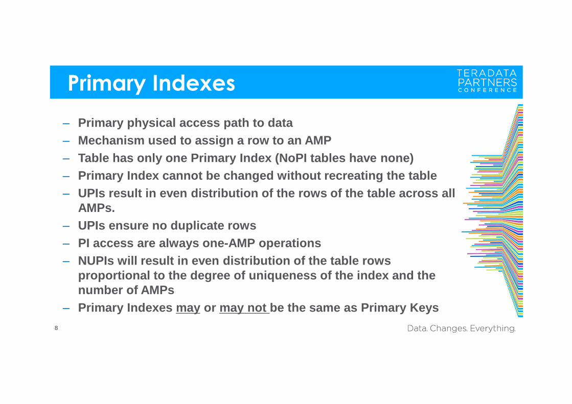
– Primary physical access path to data– Mechanism used to assign a row to an AMP– Table has only one Primary Index (NoPI tables have none)– Primary Index cannot be changed without recreating the table– UPIs result in even distribution of the rows of the table across all

AMPs.– UPIs ensure no duplicate rows – PI access are always one-AMP operations– NUPIs will result in even distribution of the table rows

proportional to the degree of uniqueness of the ind ex and the number of AMPs

– Primary Indexes may or may not be the same as Primar y Keys8

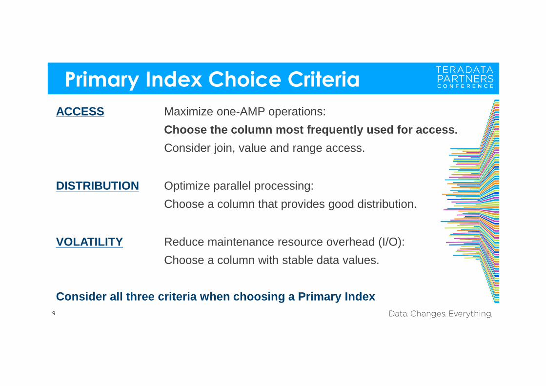
ACCESS Maximize one-AMP operations:

Choose the column most frequently used for access.

Consider join, value and range access.

DISTRIBUTION Optimize parallel processing:

Choose a column that provides good distribution.

VOLATILITY Reduce maintenance resource overhead (I/O):

Choose a column with stable data values.

Consider all three criteria when choosing a Primary Index

Primary Index Choice Criteria

9

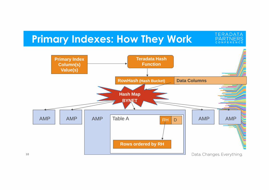
Primary Indexes: How They Work

10

Teradata Hash Function

RowHash (Hash Bucket) Data Columns

Primary Index Column(s) Value(s)

AMP AMP AMP AMPRH DTable A

Rows ordered by RH

Hash MapBYNET

AMP

Primary Index Review

11

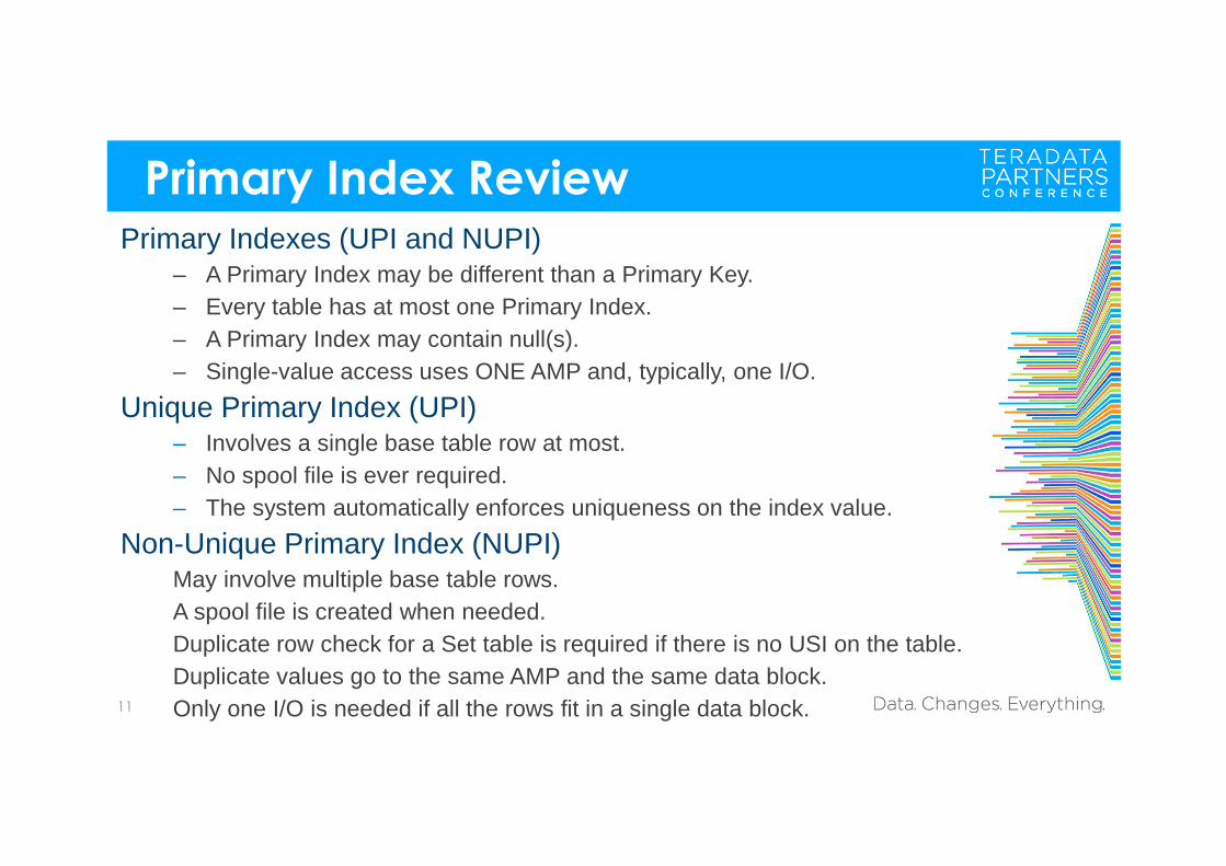
Primary Indexes (UPI and NUPI)– A Primary Index may be different than a Primary Key.– Every table has at most one Primary Index.– A Primary Index may contain null(s).– Single-value access uses ONE AMP and, typically, one I/O.

Unique Primary Index (UPI)– Involves a single base table row at most.– No spool file is ever required.– The system automatically enforces uniqueness on the index value.

Non-Unique Primary Index (NUPI)May involve multiple base table rows.A spool file is created when needed.Duplicate row check for a Set table is required if there is no USI on the table.Duplicate values go to the same AMP and the same data block.Only one I/O is needed if all the rows fit in a single data block.

Partitioned Primary Index (PPI)

12

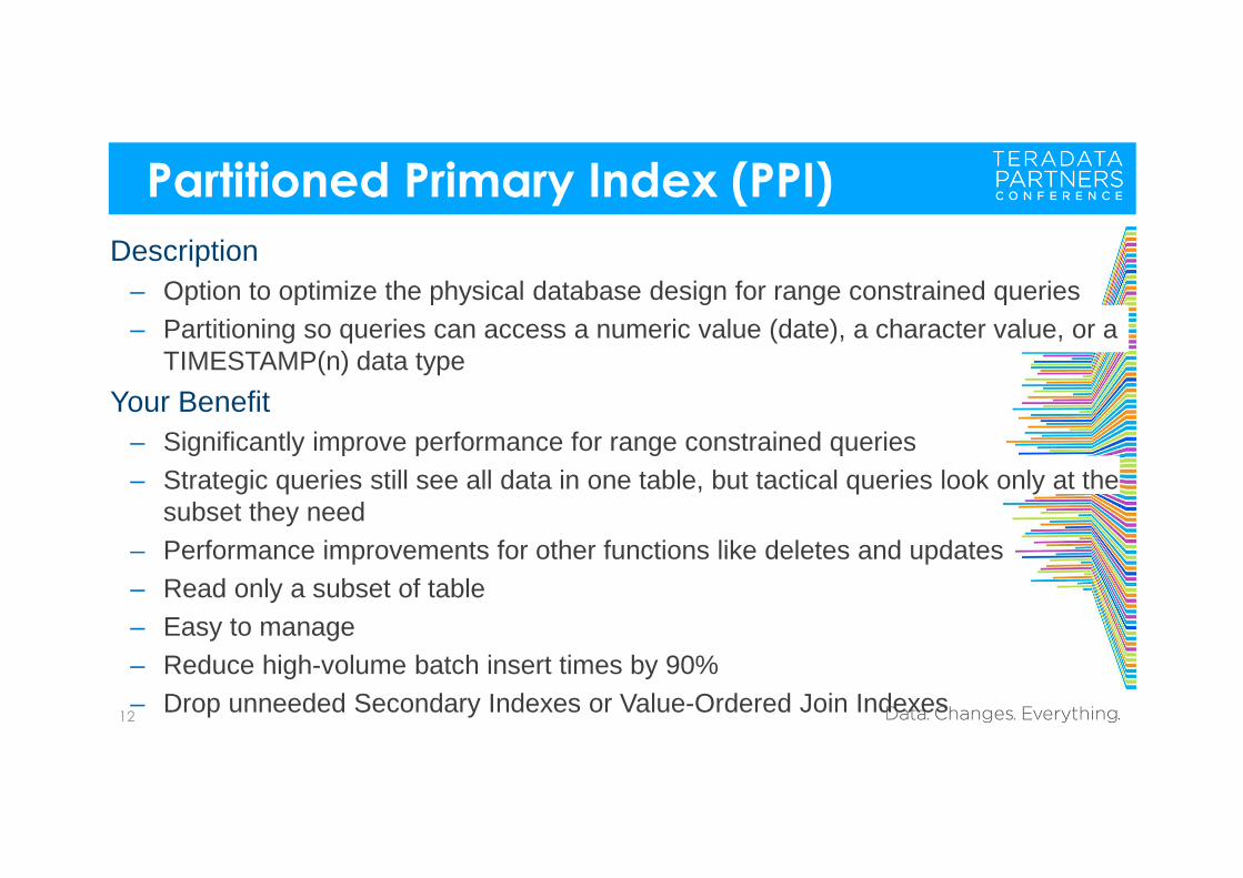
Description– Option to optimize the physical database design for range constrained queries– Partitioning so queries can access a numeric value (date), a character value, or a

TIMESTAMP(n) data type

Your Benefit – Significantly improve performance for range constrained queries– Strategic queries still see all data in one table, but tactical queries look only at the

subset they need– Performance improvements for other functions like deletes and updates – Read only a subset of table– Easy to manage– Reduce high-volume batch insert times by 90%– Drop unneeded Secondary Indexes or Value-Ordered Join Indexes


13

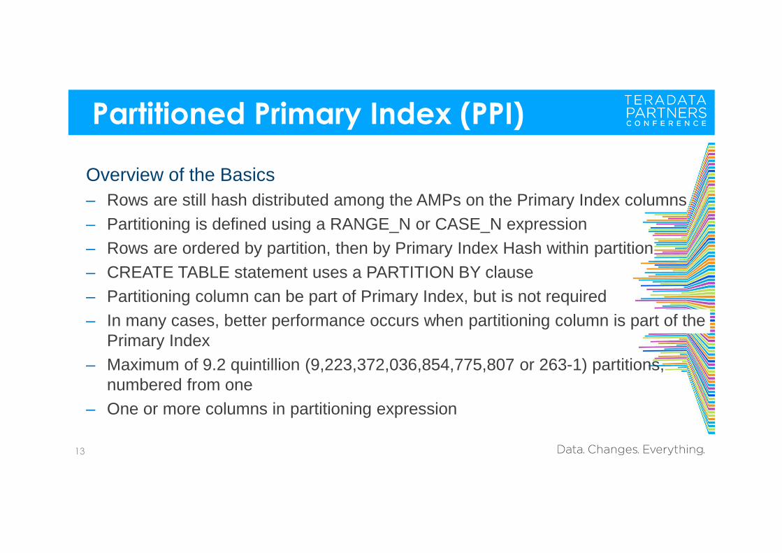
Overview of the Basics– Rows are still hash distributed among the AMPs on the Primary Index columns– Partitioning is defined using a RANGE_N or CASE_N expression– Rows are ordered by partition, then by Primary Index Hash within partition– CREATE TABLE statement uses a PARTITION BY clause– Partitioning column can be part of Primary Index, but is not required– In many cases, better performance occurs when partitioning column is part of the

Primary Index– Maximum of 9.2 quintillion (9,223,372,036,854,775,807 or 263-1) partitions,

numbered from one– One or more columns in partitioning expression


14

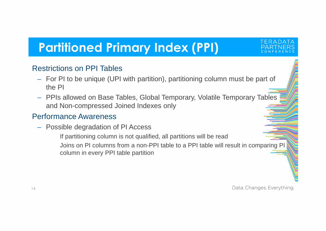
Restrictions on PPI Tables– For PI to be unique (UPI with partition), partitioning column must be part of

the PI– PPIs allowed on Base Tables, Global Temporary, Volatile Temporary Tables

and Non-compressed Joined Indexes only

Performance Awareness– Possible degradation of PI Access

If partitioning column is not qualified, all partitions will be readJoins on PI columns from a non-PPI table to a PPI table will result in comparing PI column in every PPI table partition

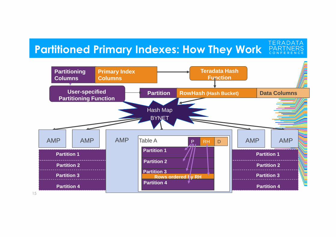
Partitioned Primary Indexes: How They Work

15

Partitioning Columns

Teradata Hash Function

Partition RowHash (Hash Bucket) Data Columns

Primary Index Columns

AMP AMP AMP AMP

User-specifiedPartitioning Function

Hash MapBYNET

P RH DTable A

Partition 1

Partition 2

Rows ordered by RHPartition 4

Partition 3

AMP

Partition 1

Partition 2

Partition 4

Partition 3

Partition 1

Partition 2

Partition 4

Partition 3

Partitioned Primary Indexes

16

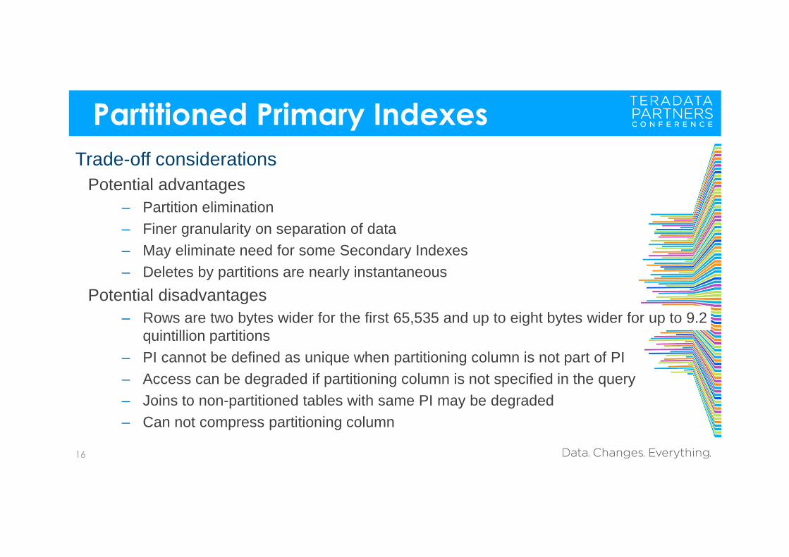
Trade-off considerationsPotential advantages

– Partition elimination– Finer granularity on separation of data– May eliminate need for some Secondary Indexes– Deletes by partitions are nearly instantaneous

Potential disadvantages– Rows are two bytes wider for the first 65,535 and up to eight bytes wider for up to 9.2

quintillion partitions– PI cannot be defined as unique when partitioning column is not part of PI– Access can be degraded if partitioning column is not specified in the query– Joins to non-partitioned tables with same PI may be degraded – Can not compress partitioning column

Partitioned Primary Indexes

17

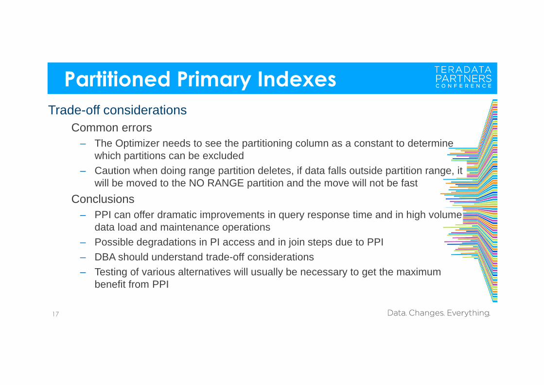
Trade-off considerationsCommon errors

– The Optimizer needs to see the partitioning column as a constant to determine which partitions can be excluded

– Caution when doing range partition deletes, if data falls outside partition range, it will be moved to the NO RANGE partition and the move will not be fast

Conclusions– PPI can offer dramatic improvements in query response time and in high volume

data load and maintenance operations– Possible degradations in PI access and in join steps due to PPI– DBA should understand trade-off considerations– Testing of various alternatives will usually be necessary to get the maximum

benefit from PPI

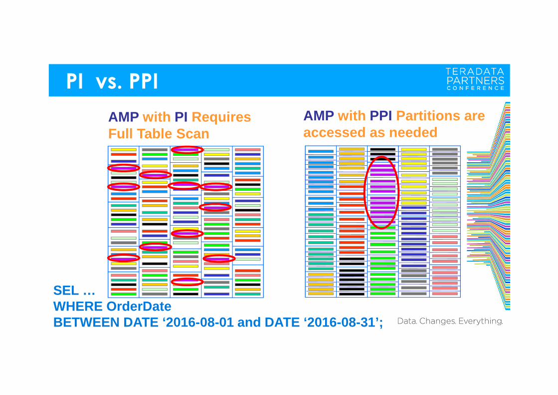
PI vs. PPI

18

SEL … WHERE OrderDate BETWEEN DATE ‘2016-08-01 and DATE ‘2016-08-31’;

AMP with PPI Partitions are accessed as needed

AMP with PI RequiresFull Table Scan

Multi-Level Partitioned Primary Index

19

DescriptionExtend Partitioned Primary Index (PPI) capability to support and allow for the creation of a table or Non-Compressed Join Index with a Multi-Level Partitioned Primary Index (ML-PPI).

BenefitThe use of ML-PPI on table(s) affords a greater opportunity for the Teradata Optimizer to achieve a greater degree of partition elimination at a more granular level which in turn results in achieving a greater level of query performance.

ConsiderationsThe Teradata Optimizer determines whether or not the Index and partitioning is usable as part of the best-cost query planning process.The Optimizer will use the Index as part of the plan to execute a given query automatically.

PPI and ML-PPI Concepts

20

Multi-level partitioning allows each partition at a level to be sub-partitioned.Each partitioning level is independently defined using a RANGE_N or CASE_N expression. Teradata combines multiple “WHERE” predicates that result in partition eliminationInternally, these range partitions are combined into a single partitioning expression that defines how the data is partitioned on the AMP.If PARTITION BY is specified for a Primary Index (PI), that PI is called a Partitioned Primary Index (PPI). If only one partitioning expression is specified, that PPI is called a single-level Partitioned Primary Index (or single-level PPI). If more than one partitioning expression is specified, that PPI is called a multi-level Partitioned Primary Index (or multi-level PPI). For PPI tables, the rows continue to be distributed across the AMPs in the same fashion, but on each AMP the rows are ordered first by partition number and then within each partition by hash. 20

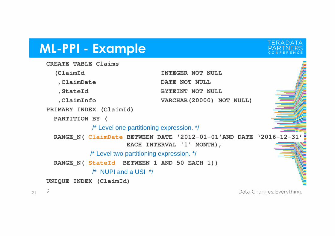
ML-PPI - Example

21

CREATE TABLE Claims

(ClaimId INTEGER NOT NULL

,ClaimDate DATE NOT NULL

,StateId BYTEINT NOT NULL

,ClaimInfo VARCHAR(20000) NOT NULL)

PRIMARY INDEX (ClaimId)

PARTITION BY (

/* Level one partitioning expression. */RANGE_N( ClaimDate BETWEEN DATE ‘2012-01-01’AND DATE ‘2016-12-31’

EACH INTERVAL '1' MONTH),

/* Level two partitioning expression. */RANGE_N( StateId BETWEEN 1 AND 50 EACH 1))

/* NUPI and a USI */UNIQUE INDEX (ClaimId)

;

ML-PPI - Example

22

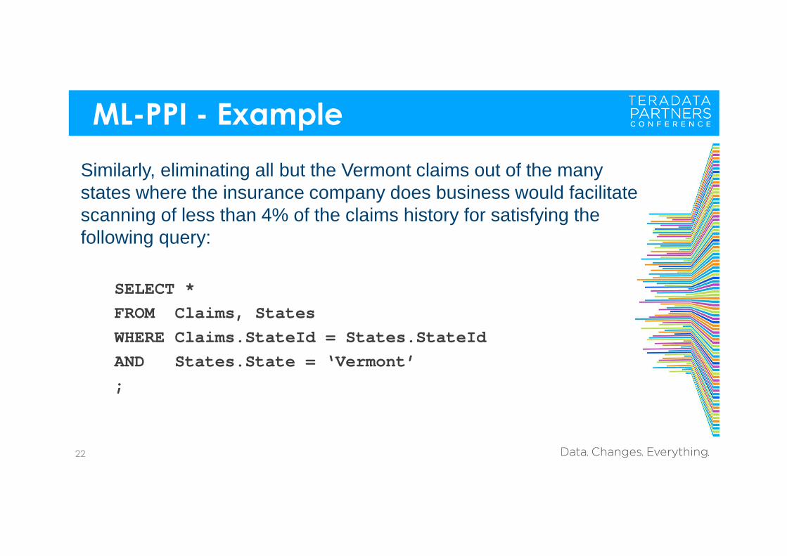
Similarly, eliminating all but the Vermont claims out of the many states where the insurance company does business would facilitate scanning of less than 4% of the claims history for satisfying the following query:

SELECT *

FROM Claims, States

WHERE Claims.StateId = States.StateId

AND States.State = ‘Vermont’

;

ML-PPI - Example

23

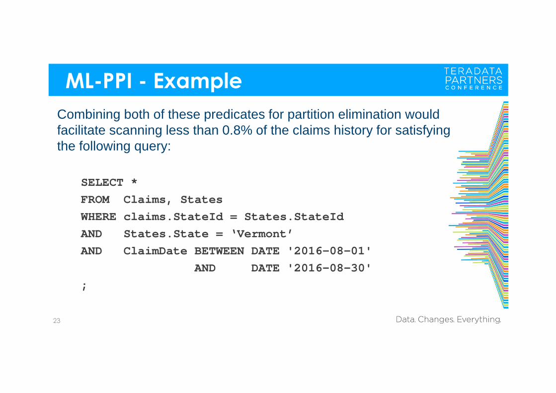
Combining both of these predicates for partition elimination would facilitate scanning less than 0.8% of the claims history for satisfying the following query:

SELECT *

FROM Claims, States

WHERE claims.StateId = States.StateId

AND States.State = ‘Vermont’

AND ClaimDate BETWEEN DATE '2016-08-01'

AND DATE '2016-08-30'

;

ML-PPI - Supported Objects

24

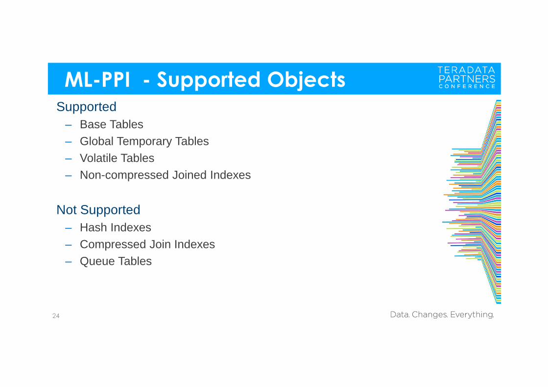
Supported– Base Tables– Global Temporary Tables– Volatile Tables– Non-compressed Joined Indexes

Not Supported– Hash Indexes– Compressed Join Indexes– Queue Tables

Secondary Indexes

• Secondary Indexes> Unique Secondary Index (USI)> Non-unique Secondary Index (NUSI)

Secondary Indexes

26

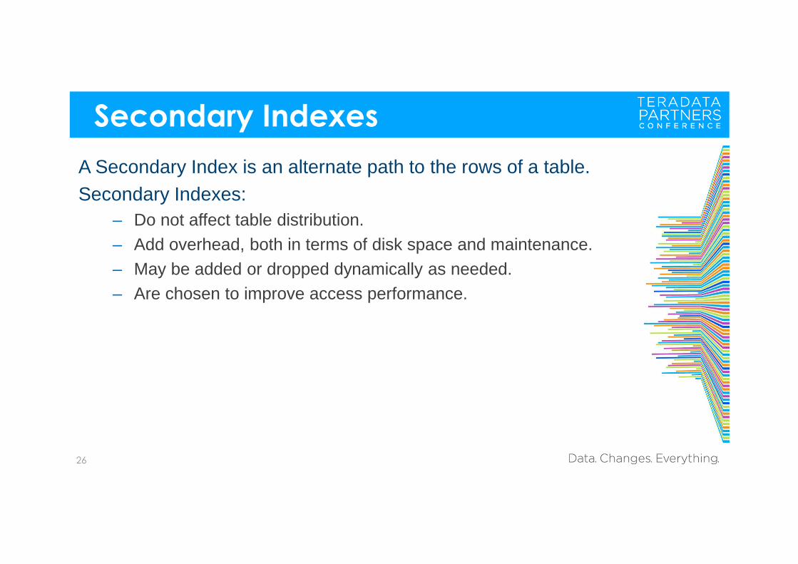
A Secondary Index is an alternate path to the rows of a table.Secondary Indexes:

– Do not affect table distribution.– Add overhead, both in terms of disk space and maintenance.– May be added or dropped dynamically as needed.– Are chosen to improve access performance.

Unique Secondary Index (USI) Access

27

Customer table Id = 100

USI Value = 54

Table ID Row Hash USI Value

100 602 54

Hashing Algorithm

PE

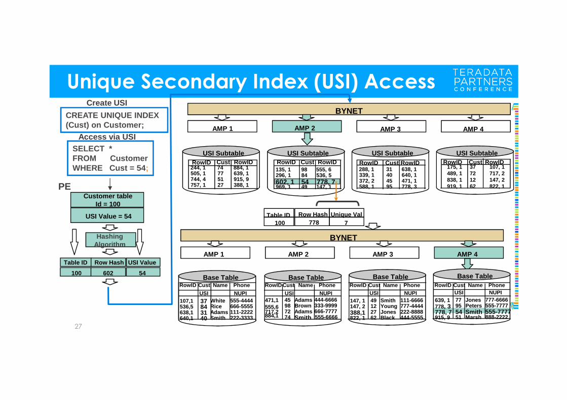
CREATE UNIQUE INDEX (Cust) on Customer;

SELECT *FROM CustomerWHERE Cust = 54 ;

Create USI

Access via USI

AMP 1 AMP 2 AMP 3 AMP 4

RowID Cust RowID RowID Cust RowID RowID Cust RowID

BYNET

AMP 2

Table ID100

Row Hash778

Unique Val7

USI Subtable USI SubtableUSI Subtable

BYNET

AMP 1 AMP 3 AMP 4

RowID Cust RowIDUSI Subtable

74775127

884, 1639, 1915, 9388, 1

244, 1505, 1744, 4757, 1

8498

5449

536, 5555, 6

778, 7147, 1

296, 1135, 1

602, 1969, 1

31404595

638, 1640, 1471, 1778, 3

288, 1339, 1372, 2588, 1

175, 1 37 107, 1489, 1 72 717, 2838, 1 12 147, 2919, 1 62 822, 1

AdamsSmith

RiceWhite 555-4444

111-2222222-3333

666-555531

37

40

84107,1536,5638,1640,1

RowID Cust Name Phone

NUPI

Base Table

USI

RowIDCust Name Phone

NUPI

Base Table

USI

Base Table Base Table

AdamsSmith

BrownAdams 444-6666

666-7777555-6666

333-999972

45

74

98471,1555,6717,2884,1

JonesBlack

YoungSmith 111-6666

222-8888444-5555

777-444427

49

62

12147, 1147, 2388,1822, 1

RowID Cust Name PhoneNUPIUSI

SmithMarsh

PetersJones 777-6666

555-7777888-2222

555-777754

77

51

95639, 1778, 3778, 7915, 9

RowID Cust Name PhoneNUPIUSI

Non-Unique Secondary Index (NUSI) Access

28

28

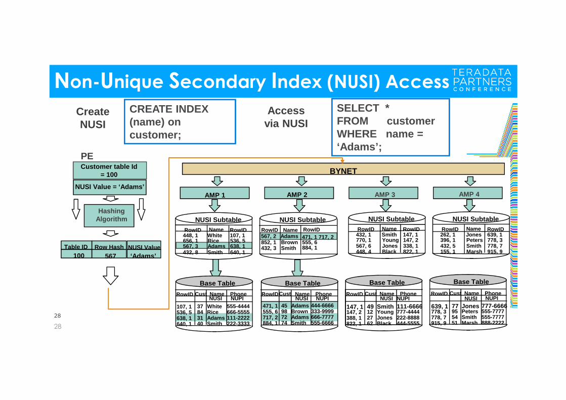
Table ID

100Row Hash

567NUSI Value‘Adams’

Hashing Algorithm

Customer table Id = 100

NUSI Value = ‘Adams’

PE

CREATE INDEX (name) on customer;

SELECT *FROM customerWHERE name = ‘Adams’;

Create NUSI

Access via NUSI

BYNET

AMP 2AMP 1

BrownAdams

Smith555, 6471, 1 717, 2

884, 1852, 1567, 2

432, 3

RowID Name RowIDWhiteRiceAdamsSmith

107, 1536, 5638, 1640, 1

448, 1656, 1567, 3432, 8

RowID Name RowID

NUSI Subtable NUSI Subtable

SmithYoungJonesBlack

147, 1147, 2338, 1822, 1

432, 1770, 1567, 6448, 4

RowID Name RowID

NUSI Subtable

JonesPetersSmithMarsh

639, 1778, 3778, 7915, 9

262, 1396, 1432, 5155, 1

RowID Name RowID

NUSI Subtable

AMP 4AMP 3

AdamsSmith

RiceWhite 555-4444

111-2222222-3333

666-555531

37

40

84107, 1536, 5638, 1640, 1

RowID Cust Name PhoneNUPI

Base Table


Base Table Base Table Base Table

AdamsSmith

BrownAdams 444-6666

666-7777555-6666

333-999972

45

74

98471, 1555, 6717, 2884, 1

JonesBlack

YoungSmith 111-6666

222-8888444-5555

777-444427

49

62

12147, 1147, 2388, 1822, 1


SmithMarsh

PetersJones 777-6666

555-7777888-2222

555-777754

77

51

95639, 1778, 3778, 7915, 9

RowID Cust Name PhoneNUPINUSI NUSI NUSI NUSI

Full Table Scans vs. Non-Unique Secondary Index (NUSI)

29

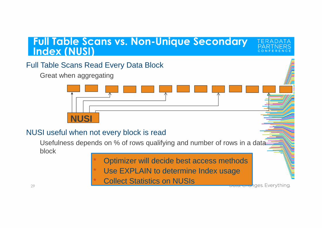
Full Table Scans Read Every Data BlockGreat when aggregating

NUSI useful when not every block is read Usefulness depends on % of rows qualifying and number of rows in a data block

* Optimizer will decide best access methods* Use EXPLAIN to determine Index usage* Collect Statistics on NUSIs

NUSI

NUSI on PI Columns of PPI Table

30

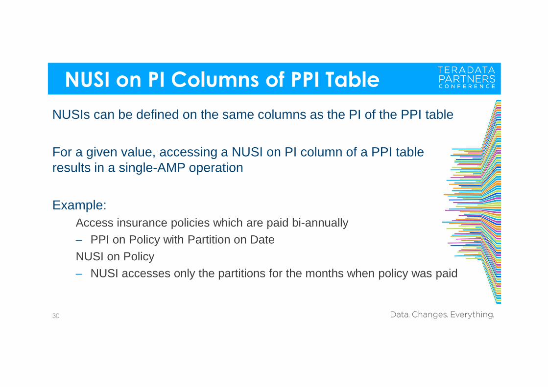
NUSIs can be defined on the same columns as the PI of the PPI table

For a given value, accessing a NUSI on PI column of a PPI table results in a single-AMP operation

Example:Access insurance policies which are paid bi-annually– PPI on Policy with Partition on DateNUSI on Policy– NUSI accesses only the partitions for the months when policy was paid

USI on PI Columns of PPI Table

31

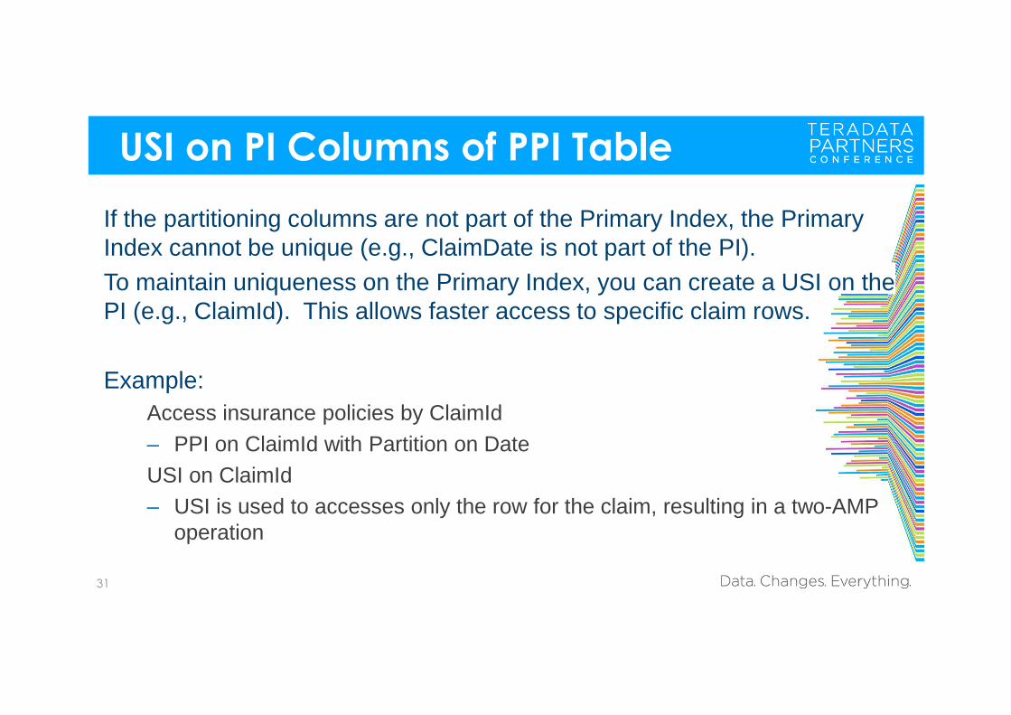
If the partitioning columns are not part of the Primary Index, the Primary Index cannot be unique (e.g., ClaimDate is not part of the PI).To maintain uniqueness on the Primary Index, you can create a USI on the PI (e.g., ClaimId). This allows faster access to specific claim rows.

Example:Access insurance policies by ClaimId– PPI on ClaimId with Partition on DateUSI on ClaimId– USI is used to accesses only the row for the claim, resulting in a two-AMP

operation

Secondary Index Review

32

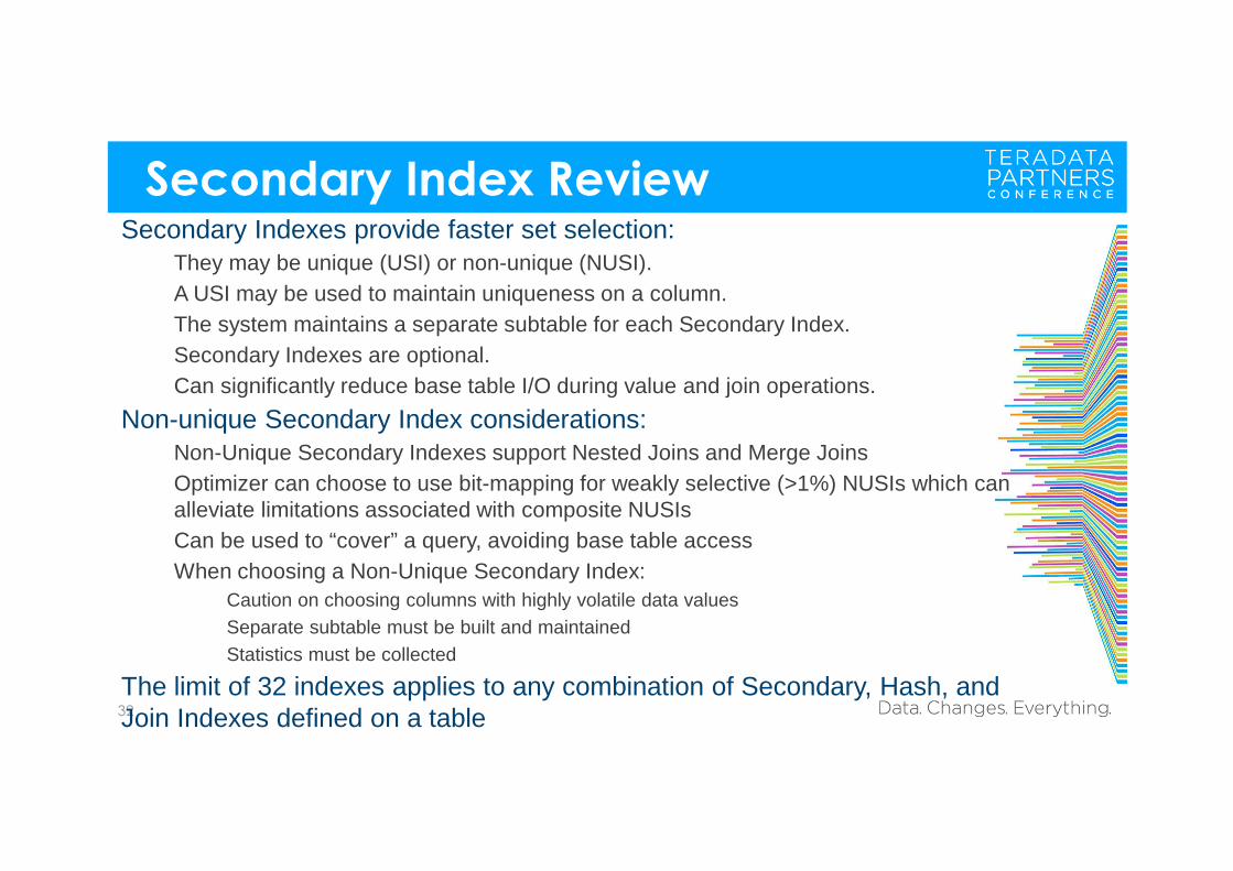
Secondary Indexes provide faster set selection:They may be unique (USI) or non-unique (NUSI).A USI may be used to maintain uniqueness on a column.The system maintains a separate subtable for each Secondary Index.Secondary Indexes are optional. Can significantly reduce base table I/O during value and join operations.

Non-unique Secondary Index considerations:Non-Unique Secondary Indexes support Nested Joins and Merge JoinsOptimizer can choose to use bit-mapping for weakly selective (>1%) NUSIs which can alleviate limitations associated with composite NUSIsCan be used to “cover” a query, avoiding base table accessWhen choosing a Non-Unique Secondary Index:

Caution on choosing columns with highly volatile data valuesSeparate subtable must be built and maintainedStatistics must be collected

The limit of 32 indexes applies to any combination of Secondary, Hash, and Join Indexes defined on a table

Other Indexes

More Indexes

• Single Table Join Index• Value Ordered Index• Sparse Join Index• Value Ordered Sparse Single Table Join Index

Other Indexes

34

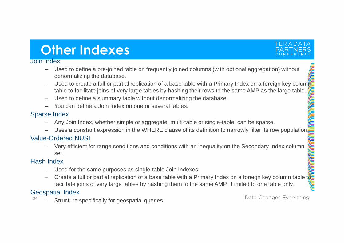
Join Index – Used to define a pre-joined table on frequently joined columns (with optional aggregation) without

denormalizing the database.– Used to create a full or partial replication of a base table with a Primary Index on a foreign key column

table to facilitate joins of very large tables by hashing their rows to the same AMP as the large table.– Used to define a summary table without denormalizing the database.– You can define a Join Index on one or several tables.

Sparse Index– Any Join Index, whether simple or aggregate, multi-table or single-table, can be sparse. – Uses a constant expression in the WHERE clause of its definition to narrowly filter its row population.

Value-Ordered NUSI– Very efficient for range conditions and conditions with an inequality on the Secondary Index column

set.

Hash Index– Used for the same purposes as single-table Join Indexes.– Create a full or partial replication of a base table with a Primary Index on a foreign key column table to

facilitate joins of very large tables by hashing them to the same AMP. Limited to one table only.

Geospatial Index– Structure specifically for geospatial queries

Join Indexes

35

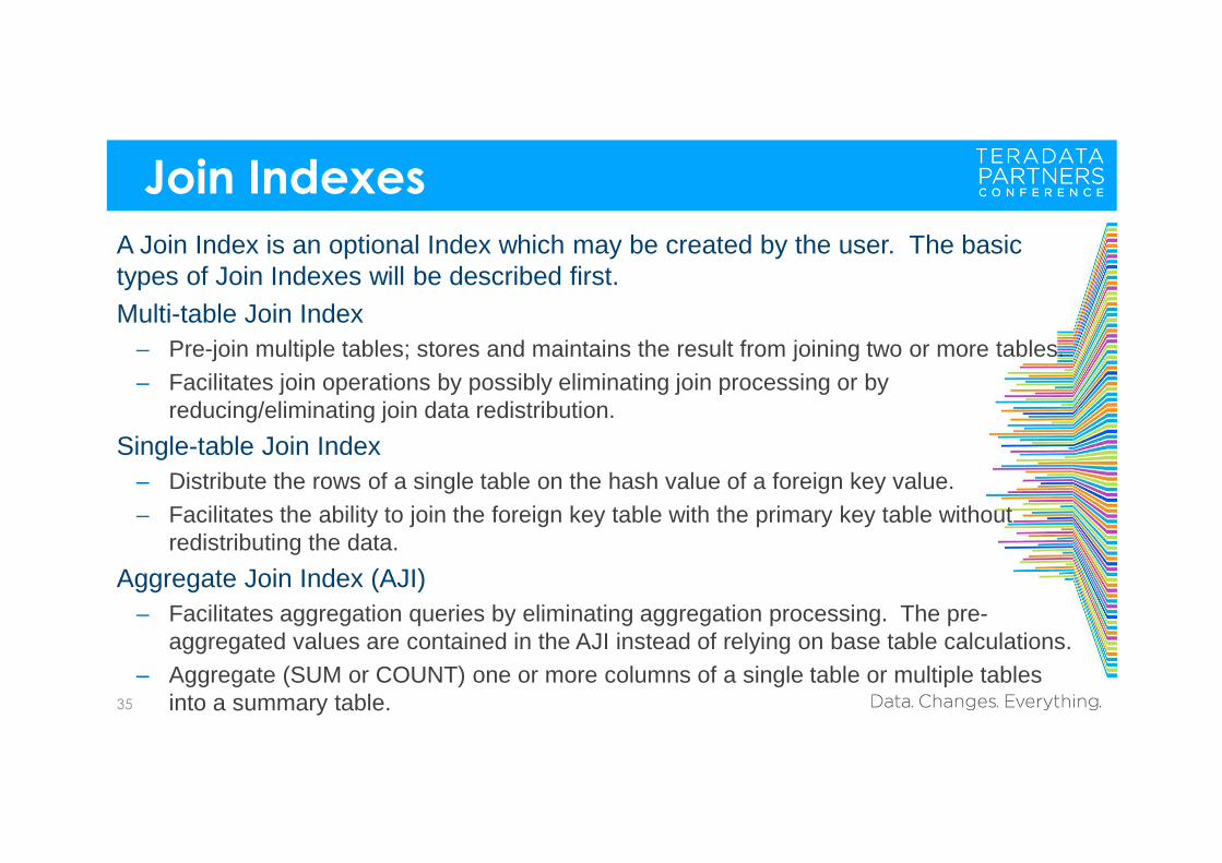
A Join Index is an optional Index which may be created by the user. The basic types of Join Indexes will be described first.Multi-table Join Index

– Pre-join multiple tables; stores and maintains the result from joining two or more tables.– Facilitates join operations by possibly eliminating join processing or by

reducing/eliminating join data redistribution.

Single-table Join Index– Distribute the rows of a single table on the hash value of a foreign key value.– Facilitates the ability to join the foreign key table with the primary key table without

redistributing the data.

Aggregate Join Index (AJI)– Facilitates aggregation queries by eliminating aggregation processing. The pre-

aggregated values are contained in the AJI instead of relying on base table calculations.– Aggregate (SUM or COUNT) one or more columns of a single table or multiple tables

into a summary table.

Single Table Join Index (STJI)

36

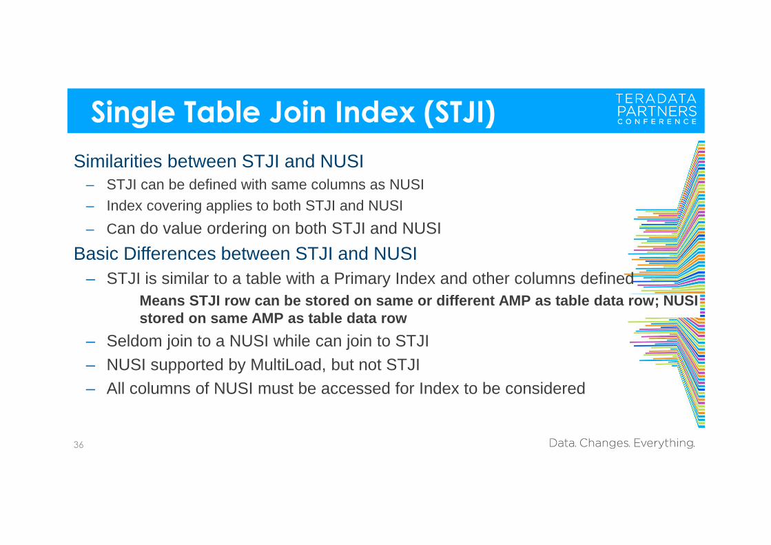
Similarities between STJI and NUSI– STJI can be defined with same columns as NUSI– Index covering applies to both STJI and NUSI

– Can do value ordering on both STJI and NUSI

Basic Differences between STJI and NUSI– STJI is similar to a table with a Primary Index and other columns defined

Means STJI row can be stored on same or different A MP as table data row; NUSI stored on same AMP as table data row

– Seldom join to a NUSI while can join to STJI– NUSI supported by MultiLoad, but not STJI – All columns of NUSI must be accessed for Index to be considered

Single Table Join Index (STJI) – Same Primary Index – Partial Covering

37

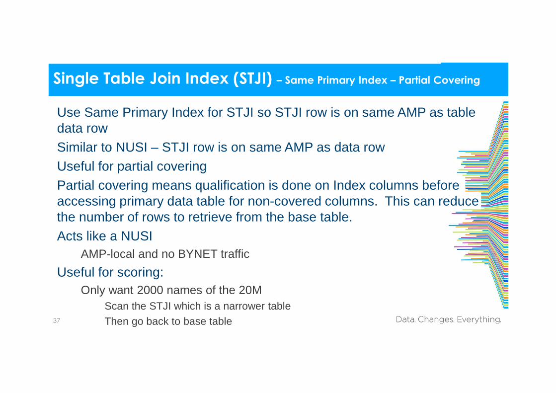
Use Same Primary Index for STJI so STJI row is on same AMP as table data rowSimilar to NUSI – STJI row is on same AMP as data rowUseful for partial coveringPartial covering means qualification is done on Index columns before accessing primary data table for non-covered columns. This can reduce the number of rows to retrieve from the base table.Acts like a NUSI

AMP-local and no BYNET traffic

Useful for scoring:Only want 2000 names of the 20M

Scan the STJI which is a narrower tableThen go back to base table

STJI - Using LIKE clause

38

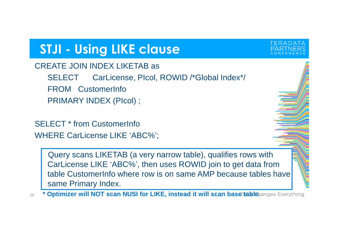
CREATE JOIN INDEX LIKETAB asSELECT CarLicense, PIcol, ROWID /*Global Index*/FROM CustomerInfoPRIMARY INDEX (PIcol) ;

SELECT * from CustomerInfoWHERE CarLicense LIKE ‘ABC%’;

Query scans LIKETAB (a very narrow table), qualifies rows with CarLicense LIKE ‘ABC%’, then uses ROWID join to get data from table CustomerInfo where row is on same AMP because tables have same Primary Index.

* Optimizer will NOT scan NUSI for LIKE, instead it will scan base table.

Value Ordered Indexes

39

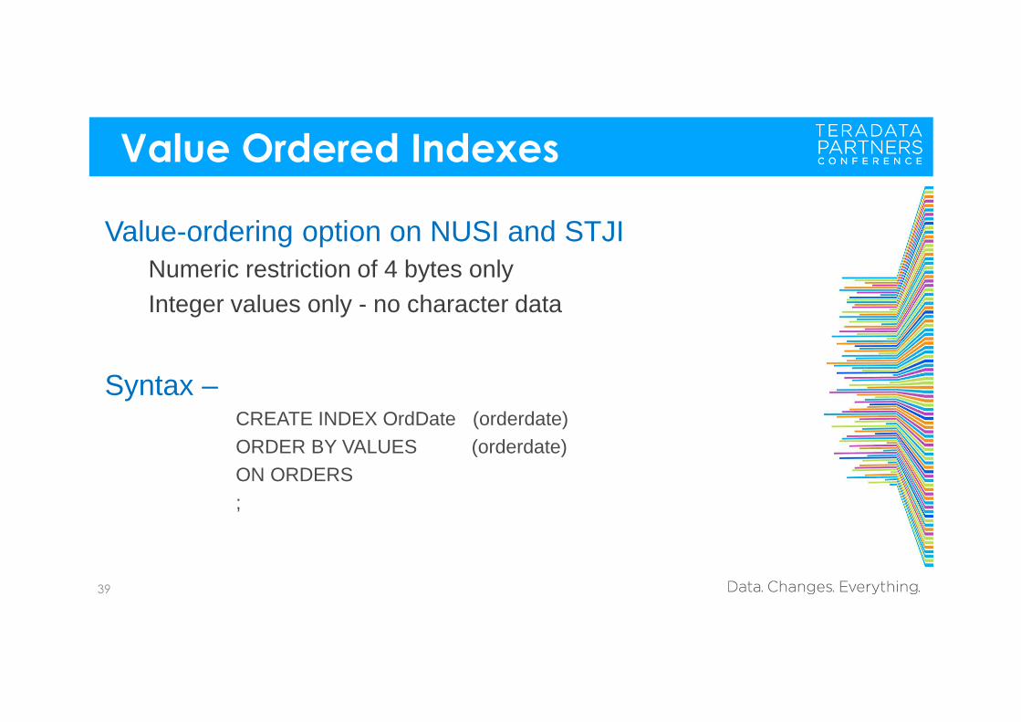
Value-ordering option on NUSI and STJINumeric restriction of 4 bytes onlyInteger values only - no character data

Syntax –CREATE INDEX OrdDate (orderdate)ORDER BY VALUES (orderdate)ON ORDERS;


40

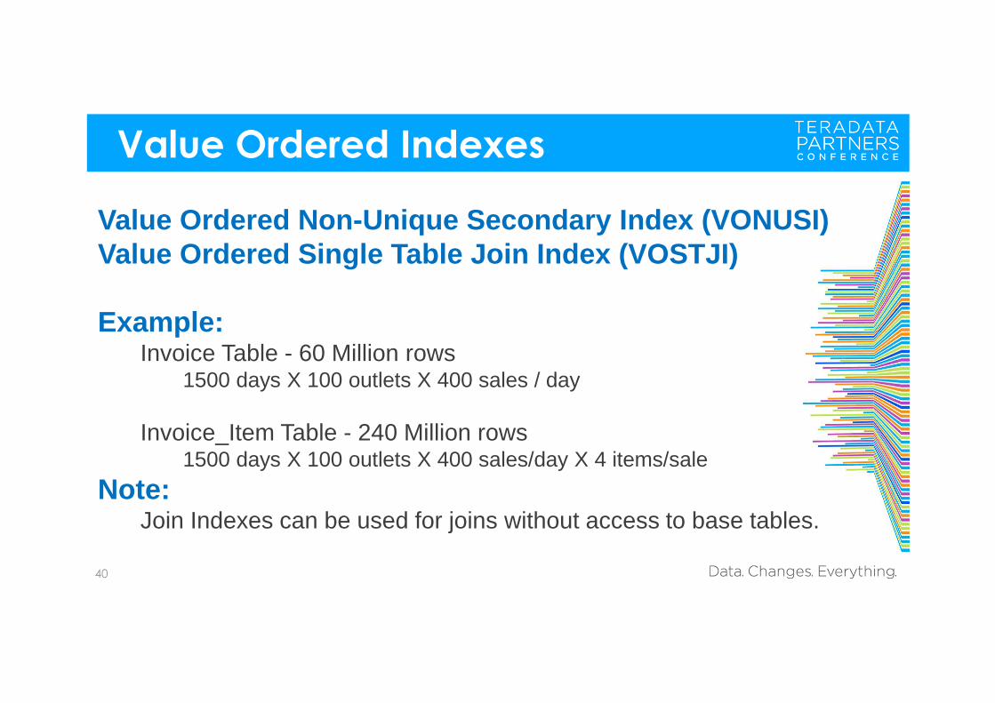
Value Ordered Non-Unique Secondary Index (VONUSI)Value Ordered Single Table Join Index (VOSTJI)

Example:Invoice Table - 60 Million rows

1500 days X 100 outlets X 400 sales / day

Invoice_Item Table - 240 Million rows1500 days X 100 outlets X 400 sales/day X 4 items/sale

Note:Join Indexes can be used for joins without access to base tables.


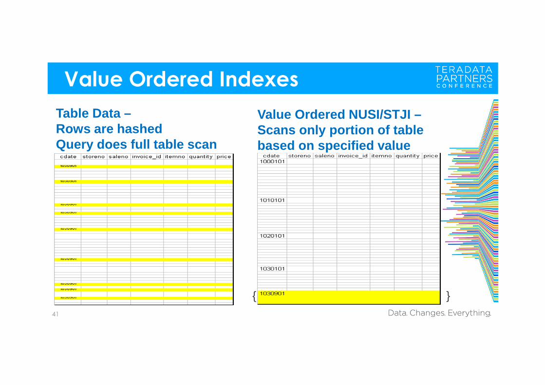
41

Value Ordered NUSI/STJI –Scans only portion of table based on specified value

Table Data –Rows are hashedQuery does full table scan

}{

Sparse Join Indexes

42

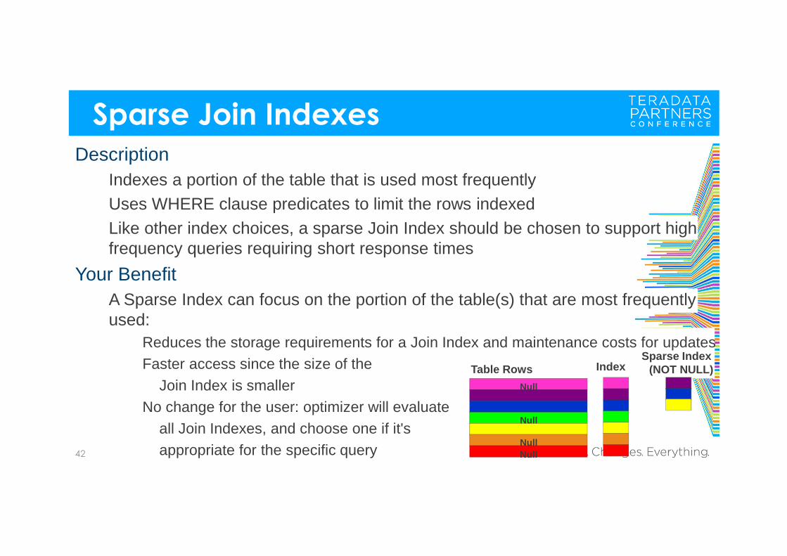
DescriptionIndexes a portion of the table that is used most frequentlyUses WHERE clause predicates to limit the rows indexedLike other index choices, a sparse Join Index should be chosen to support high frequency queries requiring short response times

Your Benefit A Sparse Index can focus on the portion of the table(s) that are most frequently used:

Reduces the storage requirements for a Join Index and maintenance costs for updatesFaster access since the size of the

Join Index is smallerNo change for the user: optimizer will evaluate

all Join Indexes, and choose one if it's appropriate for the specific query 42

Table Rows Index

Null

Null

NullNull

Sparse Index (NOT NULL)

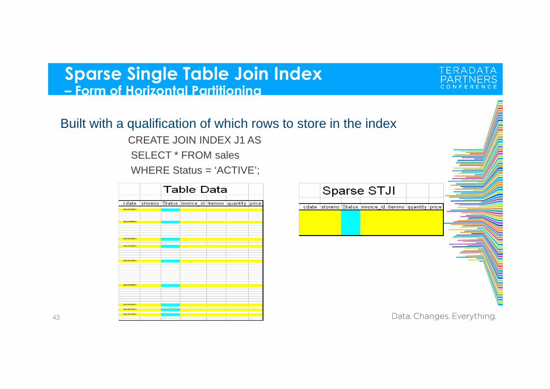
Sparse Single Table Join Index – Form of Horizontal Partitioning

43

Built with a qualification of which rows to store in the indexCREATE JOIN INDEX J1 ASSELECT * FROM salesWHERE Status = ‘ACTIVE’;

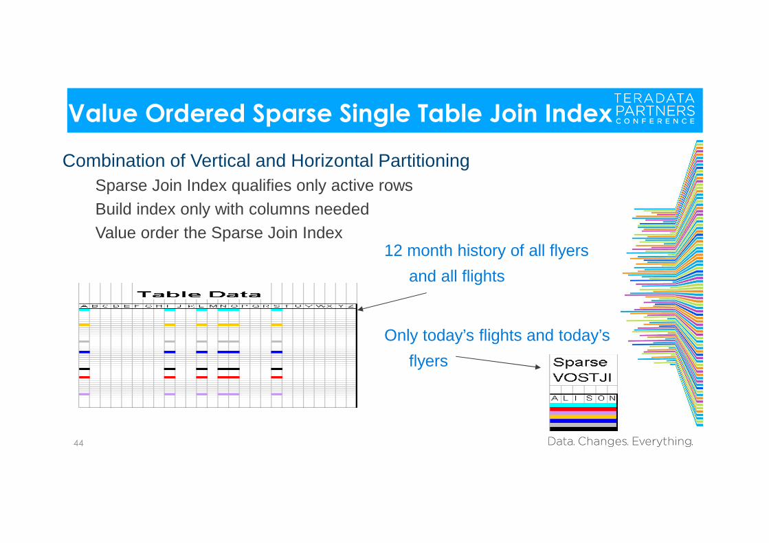
Value Ordered Sparse Single Table Join Index

44

Combination of Vertical and Horizontal PartitioningSparse Join Index qualifies only active rowsBuild index only with columns neededValue order the Sparse Join Index

12 month history of all flyers

and all flights

Only today’s flights and today’s

flyers

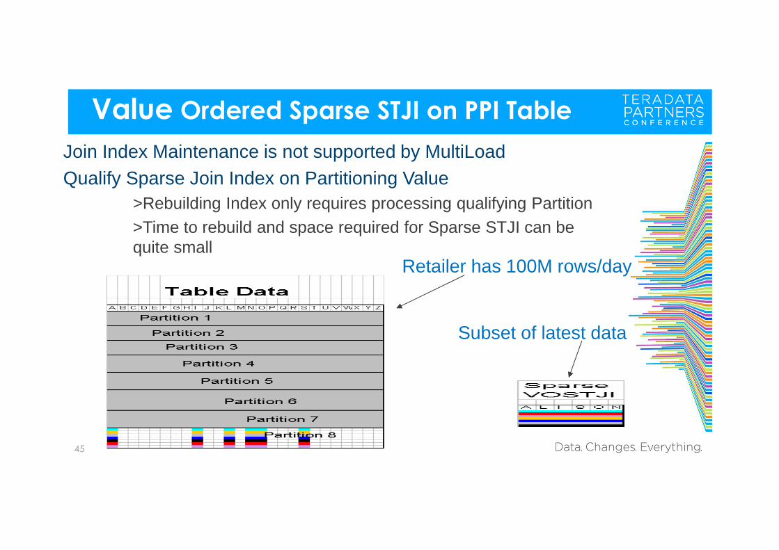
Value Ordered Sparse STJI on PPI Table

45

Join Index Maintenance is not supported by MultiLoadQualify Sparse Join Index on Partitioning Value

>Rebuilding Index only requires processing qualifying Partition >Time to rebuild and space required for Sparse STJI can be quite small

Retailer has 100M rows/day

Subset of latest data

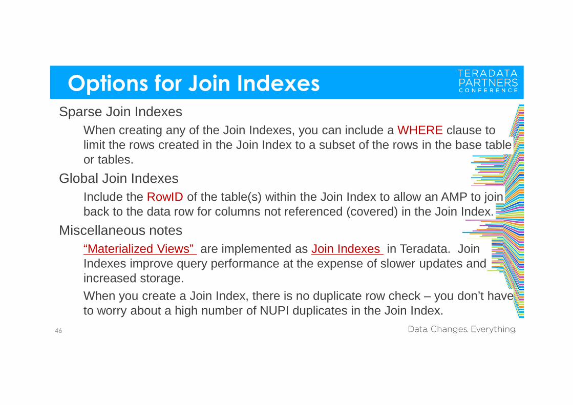
Options for Join Indexes

46

Sparse Join IndexesWhen creating any of the Join Indexes, you can include a WHERE clause to limit the rows created in the Join Index to a subset of the rows in the base table or tables.

Global Join IndexesInclude the RowID of the table(s) within the Join Index to allow an AMP to join back to the data row for columns not referenced (covered) in the Join Index.

Miscellaneous notes“Materialized Views” are implemented as Join Indexes in Teradata. Join Indexes improve query performance at the expense of slower updates and increased storage.When you create a Join Index, there is no duplicate row check – you don’t have to worry about a high number of NUPI duplicates in the Join Index.

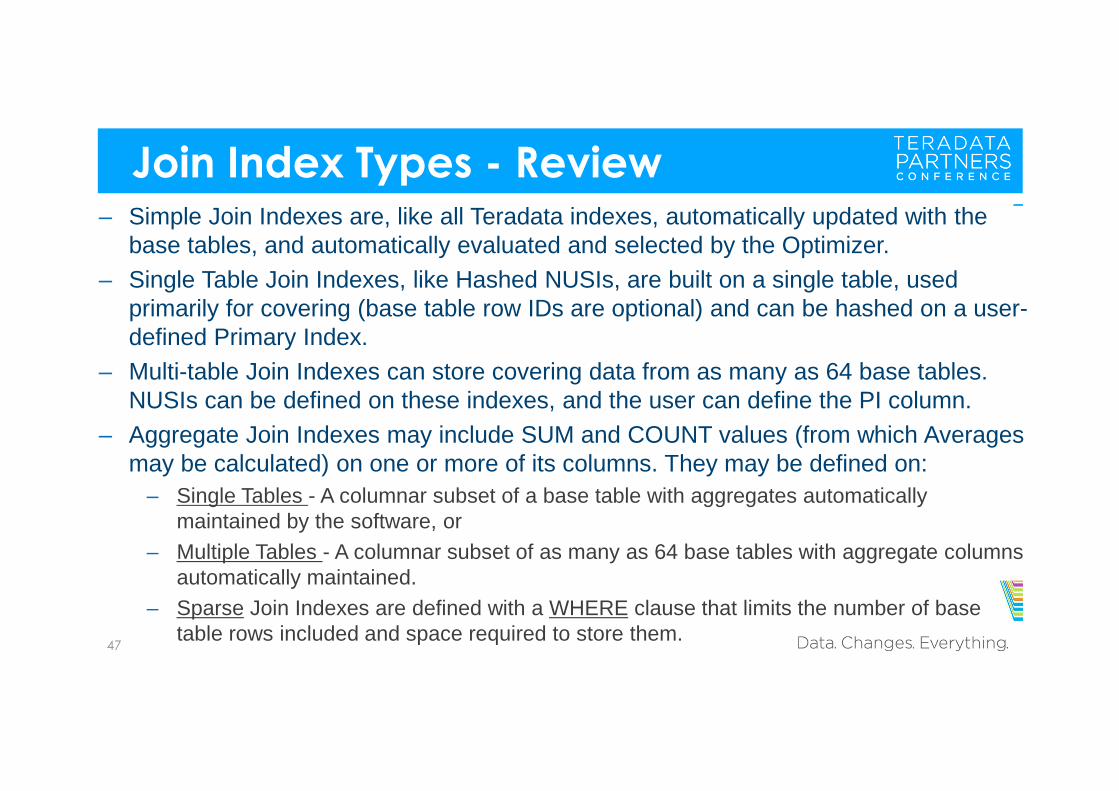
Join Index Types - Review

47

– Simple Join Indexes are, like all Teradata indexes, automatically updated with the base tables, and automatically evaluated and selected by the Optimizer.

– Single Table Join Indexes, like Hashed NUSIs, are built on a single table, used primarily for covering (base table row IDs are optional) and can be hashed on a user-defined Primary Index.

– Multi-table Join Indexes can store covering data from as many as 64 base tables. NUSIs can be defined on these indexes, and the user can define the PI column.

– Aggregate Join Indexes may include SUM and COUNT values (from which Averages may be calculated) on one or more of its columns. They may be defined on:

– Single Tables - A columnar subset of a base table with aggregates automatically maintained by the software, or

– Multiple Tables - A columnar subset of as many as 64 base tables with aggregate columns automatically maintained.

– Sparse Join Indexes are defined with a WHERE clause that limits the number of base table rows included and space required to store them.

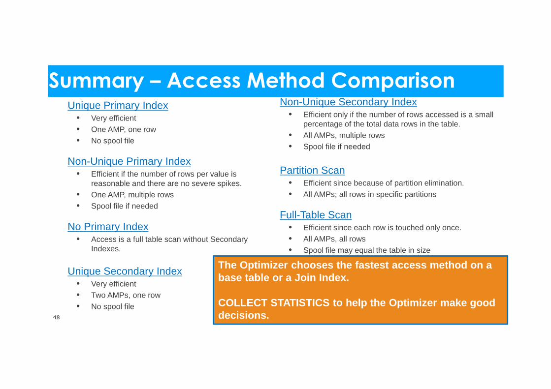
Unique Primary Index• Very efficient• One AMP, one row• No spool file

Non-Unique Primary Index• Efficient if the number of rows per value is

reasonable and there are no severe spikes.• One AMP, multiple rows• Spool file if needed

No Primary Index• Access is a full table scan without Secondary

Indexes.

Unique Secondary Index• Very efficient• Two AMPs, one row• No spool file

Non-Unique Secondary Index• Efficient only if the number of rows accessed is a small

percentage of the total data rows in the table.• All AMPs, multiple rows• Spool file if needed

Partition Scan• Efficient since because of partition elimination.• All AMPs; all rows in specific partitions

Full-Table Scan• Efficient since each row is touched only once.• All AMPs, all rows• Spool file may equal the table in size

The Optimizer chooses the fastest access method on a base table or a Join Index.

COLLECT STATISTICS to help the Optimizer make good decisions.48

Summary – Access Method Comparison

Teradata Books by Alison

Alison is the author of:Teradata ® Database Index Essentialsand Teradata ® Database EXPLAIN Essentials

The books are available online at: http://TeradataIndexes.com

Questions/CommentsEmail: [email protected]

Follow MeTwitter @ AmazingAli

Rate This Session # 0158

with the PARTNERS Mobile App

Remember To Share Your Virtual Passes

THANK YOU!

1058 Teradata Indexes How they work and when to use them …€¦ · – Capture table usage, then...

Documents

Transcript of 1058 Teradata Indexes How they work and when to use them …€¦ · – Capture table usage, then...