Bit Error Rate (BER) for BPSK modulation

by Krishna Sankar on August 5, 2007

In this post, we will derive the theoretical equation for bit error rate (BER) with Binary Phase

Shift Keying (BPSK) modulation scheme in Additive White Gaussian Noise (AWGN) channel.

The BER results obtained using Matlab/Octave simulation scripts show good agreement with the

derived theoretical results.

With Binary Phase Shift Keying (BPSK), the binary digits 1 and 0 maybe represented by the

analog levels and respectively. The system model is as shown in the Figure

below.

Figure: Simplified block diagram with BPSK transmitter-receiver

Channel Model

The transmitted waveform gets corrupted by noise , typically referred to as Additive White

Gaussian Noise (AWGN).

Additive : As the noise gets ‘added’ (and not multiplied) to the received signal

White : The spectrum of the noise if flat for all frequencies.

Gaussian : The values of the noise follows the Gaussian probability distribution function,

with and .

Computing the probability of error

Using the derivation provided in Section 5.2.1 of [COMM-PROAKIS] as reference:

The received signal,

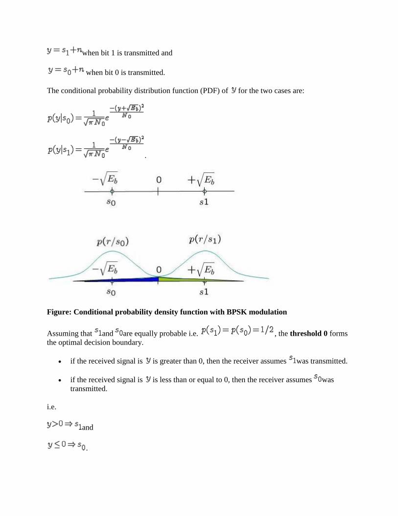
when bit 1 is transmitted and

when bit 0 is transmitted.

The conditional probability distribution function (PDF) of for the two cases are:

.

Figure: Conditional probability density function with BPSK modulation

Assuming that and are equally probable i.e. , the threshold 0 forms

the optimal decision boundary.

if the received signal is is greater than 0, then the receiver assumes was transmitted.

if the received signal is is less than or equal to 0, then the receiver assumes was

transmitted.

i.e.

and

.

Probability of error given was transmitted

With this threshold, the probability of error given is transmitted is (the area in blue region):

,

where,

is the complementary error function.

Probability of error given was transmitted

Similarly the probability of error given is transmitted is (the area in green region):

.

Total probability of bit error

.

Given that we assumed that and are equally probable i.e. , the bit

error probability is,

.

Simulation model

Matlab/Octave source code for computing the bit error rate with BPSK modulation from theory

and simulation. The code performs the following:

(a) Generation of random BPSK modulated symbols +1′s and -1′s

(b) Passing them through Additive White Gaussian Noise channel

(c) Demodulation of the received symbol based on the location in the constellation

(d) Counting the number of errors

(e) Repeating the same for multiple Eb/No value.

Figure: Bit error rate (BER) curve for BPSK modulation – theory, simulation

% Creative Commons

% Attribution-Noncommercial 2.5 India

% You are free:

% to Share — to copy, distribute and transmit the work

% to Remix — to adapt the work

% Under the following conditions:

% Attribution. You must attribute the work in the manner

% specified by the author or licensor (but not in any way

% that suggests that they endorse you or your use of the work).

% Noncommercial. You may not use this work for commercial purposes.

% For any reuse or distribution, you must make clear to others the

% license terms of this work. The best way to do this is with a

% link to this web page.

% Any of the above conditions can be waived if you get permission

% from the copyright holder.

% Nothing in this license impairs or restricts the author's moral rights.

% http://creativecommons.org/licenses/by-nc/2.5/in/

% Script for simulating binary phase shift keyed transmission and

% reception and compare the simulated and theoretical bit error

% probability

% Checked for proper operation with Octave Version 3.0.0

% Author : Krishna

% Email : krishna@dsplog.com

% Version : 1.0

% Date : 5 August 2007

% %%%%%%%%%%%%%%%%%%%%%%%%%%%%%%%%%%%%%%%%%%%%%%%%%%%%%%%%%%

clear

N = 10^6 % number of bits or symbols

rand('state',100); % initializing the rand() function

randn('state',200); % initializing the randn() function

% Transmitter

ip = rand(1,N)>0.5; % generating 0,1 with equal probability

s = 2*ip-1; % BPSK modulation 0 -> -1; 1 -> 1

n = 1/sqrt(2)*[randn(1,N) + j*randn(1,N)]; % white gaussian noise, 0dB

variance

Eb_N0_dB = [-3:10]; % multiple Eb/N0 values

for ii = 1:length(Eb_N0_dB)

% Noise addition

y = s + 10^(-Eb_N0_dB(ii)/20)*n; % additive white gaussian noise

% receiver - hard decision decoding

ipHat = real(y)>0;

% counting the errors

nErr(ii) = size(find([ip- ipHat]),2);

end

simBer = nErr/N; % simulated ber

theoryBer = 0.5*erfc(sqrt(10.^(Eb_N0_dB/10))); % theoretical ber

% plot

close all

figure

semilogy(Eb_N0_dB,theoryBer,'b.-');

hold on

semilogy(Eb_N0_dB,simBer,'mx-');

axis([-3 10 10^-5 0.5])

grid on

legend('theory', 'simulation');

xlabel('Eb/No, dB');

ylabel('Bit Error Rate');

title('Bit error probability curve for BPSK modulation');

BPSK modulation and Demodulation

April 8, 2010 in Digital Modulations, Matlab Codes, Signal Processing

BPSK Modulation:

In digital modulation techniques a set of basis functions are chosen for a particular modulation

scheme.Generally the basis functions are orthogonal to each other. Basis functions can be

derived using ‘Gram Schmidt orthogonalization‘ procedure.Once the basis function are chosen,

any vector in the signal space can be represented as a linear combination of the basis functions.

In Binary Phase Shift Keying (BPSK) only one sinusoid is taken as basis function modulation.

Modulation is achieved by varying the phase of the basis function depending on the message

bits. The following equation outlines BPSK modulation technique.

The constellation diagram of BPSK will show the constellation points lying entirely on the x

axis. It has no projection on the y axis. This means that the BPSK modulated signal will have an

in-phase component (I) but no quadrature component (Q). This is because it has only one basis

function.

A BPSK modulator can be implemented by NRZ coding the message bits (1 represented by +ve

voltage and 0 represented by -ve voltage) and multiplying the output by a reference oscillator

running at carrier frequency ω.

BPSK Modulator

BPSK Demodulation:

For BPSK demodulator , a coherent demodulator is taken as an example. In coherent detection

technique the knowledge of the carrier frequency and phase must be known to the receiver. This

can be achieved by using a Costas loop or a PLL (phase lock loop) at the receiver. A PLL

essentially locks to the incoming carrier frequency and tracks the variations in frequency and

phase. For the following simulation , neither a PLL nor a Costas loop is used but instead we

simple use the output of the PLL or Costas loop. For demonstration purposes we simply assume

that the carrier phase recovery is done and simply use the generated reference frequency at the

receiver (cos(ωt)).

In the demodulator the received signal is multiplied by a reference frequency generator

(assuming the PLL/Costas loop be present). The multiplied output is integrated over one bit

period using an integrator. A threshold detector makes a decision on each integrated bit based on

a threshold. Since an NRZ signaling format is used with equal amplitudes in positive and

negative direction, the threshold for this case would be ’0′.

BPSK Demodulator

Matlab Code:

File 1: NRZ_Encoder.m

% NRZ_Encoder Line codes e

% [time,output,Fs]=NRZ_Encod

% NRZ_Encoder NRZ encoder

% Author: Mathuranathan for h

1

2

3

4

5

6

7

8

9

10

11

12

13

% NRZ_Encoder Line codes encoder

% [time,output,Fs]=NRZ_Encoder(input,Rb,amplitude,style)

% NRZ_Encoder NRZ encoder

% Author: Mathuranathan for http://www.gaussianwaves.com

% License: Creative Commons : CC-BY-NC-SA 3.0

% Input a stream of bits and specify bit-Rate, amplitude of the output signal and the style of

encoding

% Currently 3 encoding styles are supported namely 'Manchester','Unipolar'and 'Polar'

% Outputs the NRZ stream

function [time,output,Fs]=NRZ_Encoder(input,Rb,amplitude,style)

%For debug

%clear all;

%input=[1 0 1 0 0 1 1];

14

15

16

17

18

19

20

21

22

23

24

25

26

27

28

29

30

31

32

33

34

35

36

37

38

%Tb = 0.01; % bit period (s)

%Fs = 400; % Sampling Freq Fs >=1/T (Hz)

Fs=16*Rb; %Sampling frequency , oversampling factor= 32

Ts=1/Fs; % Sampling Period

Tb=1/Rb; % Bit period

output=[];

switch lower(style)

case {'manchester'}

%disp('Method is ,manchester')

for count=1:length(input),

for tempTime=0:Ts:Tb/2-Ts,

output=[output (-1)^(input(count))*amplitude];

end

for tempTime=Tb/2:Ts:Tb-Ts,

output=[output (-1)^(input(count)+1)*amplitude];

end

end

case {'unipolar'}

%disp('Method is unipolar')

for count=1:length(input),

for tempTime=0:Ts:Tb-Ts,

output=[output input(count)*amplitude];

end

end

case {'polar'}

39

40

41

42

43

44

45

46

47

48

49

50

%disp('Method is polar')

for count=1:length(input),

for tempTime=0:Ts:Tb-Ts,

output=[output amplitude*(-1)^(1+input(count))];

end

end

otherwise,

disp('NRZ_Encoder(input,Rb,amplitude,style)-Unknown method given as ''style'' argument');

disp('Accepted Styles are ''Manchester'', ''Unipolar'' and ''Polar''');

end

time=0:Ts:Tb*length(input)-Ts;

File 2: BPSK_Mod_Demod.m

% Demonstration of BPSK Modu

% This scheme uses a simple

% random binary stream is rep

% signal is multiplied by refere

1

2

3

4

5

6

7

8

% Demonstration of BPSK Modulation and Demodulation

% This scheme uses a simple BPSK modulation scheme in which a

% random binary stream is represented in NRZ format and the resulting

% signal is multiplied by reference carrier frequency.

% AWGN channel noise generated according to the desired noise variance

% is added with the BPSK modulated signal.

% The noise added signal is demodulated by multiplying it with the

% reference frequency and integrated over one bit period.

9

10

11

12

13

14

15

16

17

18

19

20

21

22

23

24

25

26

27

28

29

30

31

32

33

%

% Author: Mathuranathan Viswanathan for http://www.gaussianwaves.com

% License : creative commons : Attribution-NonCommercial-ShareAlike 3.0

% Unported

clear; %clear all stored variables

N=100; %number of data bits

noiseVariance = 0.5; %Noise variance of AWGN channel

data=randn(1,N)>=0; %Generate uniformly distributed random data

Rb=1e3; %bit rate

amplitude=1; % Amplitude of NRZ data

[time,nrzData,Fs]=NRZ_Encoder(data,Rb,amplitude,'Polar');

Tb=1/Rb;

subplot(4,2,1);

stem(data);

xlabel('Samples');

ylabel('Amplitude');

title('Input Binary Data');

axis([0,N,-0.5,1.5]);

subplot(4,2,3);

plotHandle=plot(time,nrzData);

xlabel('Time');

ylabel('Amplitude');

title('Polar NRZ encoded data');

set(plotHandle,'LineWidth',2.5);

maxTime=max(time);

34

35

36

37

38

39

40

41

42

43

44

45

46

47

48

49

50

51

52

53

54

55

56

57

58

maxAmp=max(nrzData);

minAmp=min(nrzData);

axis([0,maxTime,minAmp-1,maxAmp+1]);

grid on;

Fc=2*Rb;

osc = sin(2*pi*Fc*time);

%BPSK modulation

bpskModulated = nrzData.*osc;

subplot(4,2,5);

plot(time,bpskModulated);

xlabel('Time');

ylabel('Amplitude');

title('BPSK Modulated Data');

maxTime=max(time);

maxAmp=max(nrzData);

minAmp=min(nrzData);

axis([0,maxTime,minAmp-1,maxAmp+1]);

%plotting the PSD of BPSK modulated data

subplot(4,2,7);

h=spectrum.welch; %Welch spectrum estimator

Hpsd = psd(h,bpskModulated,'Fs',Fs);

plot(Hpsd);

title('PSD of BPSK modulated Data');

%-------------------------------------------

%Adding Channel Noise

59

60

61

62

63

64

65

66

67

68

69

70

71

72

73

74

75

76

77

78

79

80

81

82

83

%-------------------------------------------

noise = sqrt(noiseVariance)*randn(1,length(bpskModulated));

received = bpskModulated + noise;

subplot(4,2,2);

plot(time,received);

xlabel('Time');

ylabel('Amplitude');

title('BPSK Modulated Data with AWGN noise');

%-------------------------------------------

%BPSK Receiver

%-------------------------------------------

%Multiplying the received signal with reference Oscillator

v = received.*osc;

%Integrator

integrationBase = 0:1/Fs:Tb-1/Fs;

for i = 0:(length(v)/(Tb*Fs))-1,

y(i+1)=trapz(integrationBase,v(int32(i*Tb*Fs+1):int32((i+1)*Tb*Fs)));

end

%Threshold Comparator

estimatedBits=(y>=0);

subplot(4,2,4);

stem(estimatedBits);

xlabel('Samples');

ylabel('Amplitude');

title('Estimated Binary Data');

84

85

86

87

88

89

90

91

92

93

94

95

96

97

98

99

100

101

102

103

104

105

106

107

108

axis([0,N,-0.5,1.5]);

%------------------------------------------

%Bit Error rate Calculation

BER = sum(xor(data,estimatedBits))/length(data);

%disp(BER);

%Constellation Mapping at transmitter and receiver

%constellation Mapper at Transmitter side

subplot(4,2,6);

Q = zeros(1,length(nrzData)); %No Quadrature Component for BPSK

stem(nrzData,Q);

xlabel('Inphase Component');

ylabel('Quadrature Phase component');

title('BPSK Constellation at Transmitter');

axis([-1.5,1.5,-1,1]);

%constellation Mapper at receiver side

subplot(4,2,8);

Q = zeros(1,length(y)); %No Quadrature Component for BPSK

stem(y/max(y),Q);

xlabel('Inphase Component');

ylabel('Quadrature Phase component');

title(['BPSK Constellation at Receiver when AWGN Noise Variance =',num2str(noiseVariance)]);

axis([-1.5,1.5,-1,1]);

109

110

111

112

113

114

115

Simulation Results

The output of the Matlab code provides more insight into the modulation techniques. Apart from

plotting the modulated and demodulated signal it also shows the constellation at

transmitter/receiver and Power Spectral Density of the BPSK modulated signal.

BPSK Modulation and Demodulation Characteristics