10:30 - 11:15: Reflectance Rendering with Point...
131
60 Physically Physically- Based Reflectance Based Reflectance for Games for Games 10:30 10:30 - 11:15: Reflectance 11:15: Reflectance Rendering with Point Lights Rendering with Point Lights Naty Hoffman Naty Hoffman & Dan Baker Dan Baker
Transcript of 10:30 - 11:15: Reflectance Rendering with Point...

60
PhysicallyPhysically--Based Reflectance Based Reflectance for Gamesfor Games
10:30 10:30 -- 11:15: Reflectance 11:15: Reflectance Rendering with Point LightsRendering with Point Lights
Naty HoffmanNaty Hoffman && Dan BakerDan Baker

61
Reflectance Rendering with Point Reflectance Rendering with Point LightsLights
• Analytical BRDFs (Naty & Dan)
• Other Types of BRDFs (Dan)
• Anti-Aliasing and Level-of-Detail (Dan)
In this section, we shall discuss the practical considerations for rendering reflectance models with point lights. First we will cover the most relevant analytical BRDF models, discussing implementation and production considerations for rendering each with point lights. Next we will discuss non-analytical (hand-painted and measured) BRDF models and their implementation and production considerations for rendering with point lights. Finally, we shall discuss issues relating to anti-aliasing and level-of-detail for reflection models, as rendered with point lights.

62
Analytical BRDFsAnalytical BRDFs
• Common Models (Naty)
• Implementation and Performance (Dan)
• Production Issues (Dan)
First, we shall discuss common reflection models used for rendering with point lights. Then, we discuss implementation and performance issues for these models. Finally, we discuss specific game production issues relating to these models.
63
Analytical BRDFs with Point LightsAnalytical BRDFs with Point Lights
• Typically directly evaluated in shaders
• Requirements for BRDFs are different than for Monte Carlo ray-tracers– Which require the BRDF to be strictly energy
conserving and amenable to importance sampling
• Important factors:– Ease of evaluation, meaningful parameters
Global illumination rendering algorithms have specific requirements from BRDFs. Real-time rendering, in particular direct evaluation of BRDFs with point lights, has quite different requirements. We have discussed in previous sections the importance of having BRDF parameters map to physically meaningful values.

64
Reflectance ModelsReflectance Models
• Phong
• Blinn-Phong
• Cook-Torrance
• Banks
• Ward
• Ashikhmin-Shirley
• Lafortune
• Oren-Nayar
These are the reflection models we will be discussing. This collage is composed of pieces of images that we shall see (with attributions) in the following section of the talk.

65
PhongPhong
• Commonly encountered form (sans ambient term)
• What is the physical meaning and correct range of parameters ks, kd and n?
( ) ( )( )nrsldlle kkdiL αθ coscos +=
We write this as a point-light lighting equation using ‘game intensity’, which is the most common usage. The significance and physical interpretation of the parameters is unclear, which makes them hard to set properly.

66
PhongPhong
• Written as a BRDF– We can see that the first term is essentially identical to a
Lambert BRDF
( ) ( )i
nrsd
eirkkf
θπα
πωω
coscos, +=
Comparing the previous Phong lighting equation to the “game point lights” version of the rendering equation we saw previously, we can rewrite the Phong reflection model in BRDF form. In this form, the meaning of kd is clear:
67
PhongPhong
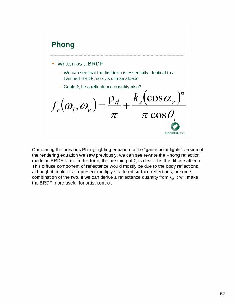
• Written as a BRDF– We can see that the first term is essentially identical to a
Lambert BRDF, so kd is diffuse albedo
– Could ks be a reflectance quantity also?
( ) ( )i
nrsd
eirkf
θπα
πωω
coscosρ, +=
Comparing the previous Phong lighting equation to the “game point lights” version of the rendering equation we saw previously, we can see rewrite the Phong reflection model in BRDF form. In this form, the meaning of kd is clear: it is the diffuse albedo. This diffuse component of reflectance would mostly be due to the body reflections, although it could also represent multiply-scattered surface reflections, or some combination of the two. If we can derive a reflectance quantity from ks, it will make the BRDF more useful for artist control.
68
PhongPhong
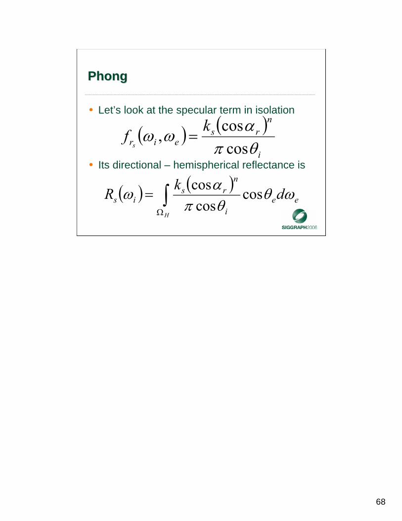
• Let’s look at the specular term in isolation
• Its directional – hemispherical reflectance is
( ) ( )i
nrs
eirkf
s θπαωω
coscos, =
( ) ( )ee
i
nrs
is dkRH
ωθθπαω cos
coscos
∫Ω
=

69
PhongPhong
• Or:
• Goes to infinity at grazing angles – not good!
• Surfaces using this BRDF will be too bright and appear to ‘glow’ at grazing angles
( ) ( ) een
ri
sis dkR
H
ωθαθπ
ω coscoscos ∫
Ω
=
For real-time rendering, we don’t need strict conservation of energy, so we don’t need the directional-hemispherical reflectance to be strictly equal or less than 1.0.However, a BRDF where the reflectance goes to infinity is going to be noticeably wrong visually.

70
PhongPhong
• First step in making the Phong specular term physically plausible, with the goal of more realistic visuals – remove the cosine factor:
• Or include a cosine factor in the original form
( ) ( )nrs
eirkf
sα
πωω cos, =
( ) ( )( )ln
rsldlle kkdiL θαθ coscoscos +=
The only reason we had an inverse cosine factor in the BRDF in the first place was the lack of a cosine factor in the specular term in the original form of the reflectance model. Once we add that, the inverse cosine factor is removed from the BRDF. This has several good effects.

71
PhongPhong
• More physically plausible
( ) ( ) een
rs
is dkRH
ωθαπ
ω coscos∫Ω
=
( )( ) ( )2
20max+
==n
kRR ssis ω
The new specular term is more physically plausible. For one thing, it is now reciprocal. This is not an important thing in itself for real-time rendering (it is for some ray-tracing algorithms) but it gives us a better feeling about the BRDF being a good model of physical reality. More importantly, it is now possible to normalize the BRDF and get one which is energy-conserving, and more importantly still, has meaningful reflectance parameters.The directional-hemispherical reflectance of the specular term is now greatest at normal incidence (when the angle of incidence is 0). If we assume that this is the Fresnel reflectance of the substance from which the surface is composed, then this makes sense. The decrease of reflectance towards glancing angles could be seen as a simulation of shadowing and masking effects. Taking this value as being equal to the Fresnel reflectance at normal incidence RF(0), we get a new form of the Phong specular term:

72
PhongPhong
• Instead of the mysterious ks, we now have RF(0)
• The (n+2)/2π term is a normalization factor
• n can be seen as controlling surface roughness
• Now artist can control specular reflectance and roughness separately
( ) ( )( )nrFeir Rnfs
απ
ωω cos02
2, +=
Instead of a mysterious ks term, we now have RF(0), the Fresnel reflectance of the surface substance at normal incidence, which is physically meaningful. We know values are appropriate to assign to RF(0) for various kinds of materials. This form of the specular term has several advantages: if we expose RF(0) and n as shader parameters, the artist can control the specular reflectance and roughness directly, changing one without changing the other. For high values of n, the normalization term will cause the BRDF to reach large values towards the center of the highlight, which is correct (the original form of the Phong term never exceeded a value of 1).

73
PhongPhong
• Complete normalized BRDF
• If ρd + RF(0) ≤ 1 at all frequencies, the BRDF will conserve energy
( ) ( )( )nrFd
eir Rnf αππ
ωω cos02
2ρ, ++=
Energy conservation can be a good guideline to setting BRDF parameters. In this case, if the artist wishes to ensure realism, they would not set the reflectance parameters to add up to more than 1 so the surface would not appear to “glow”(emit more energy than it receives).
74
PhongPhong
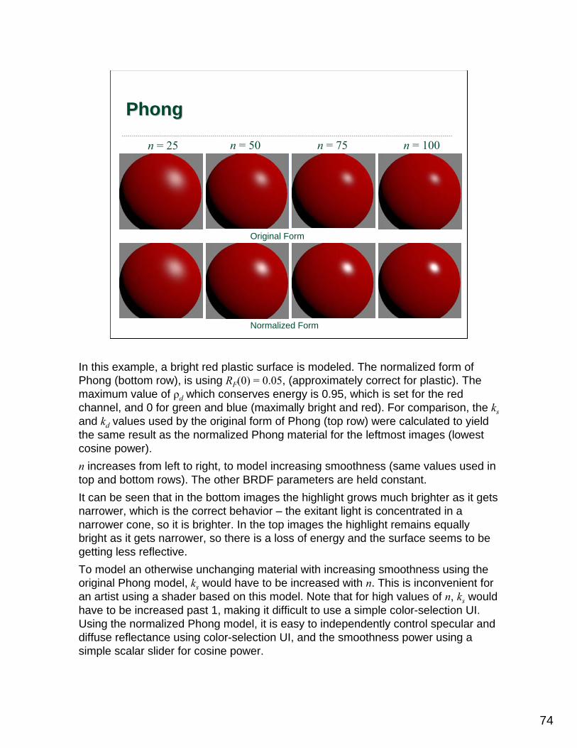
Original Form
Normalized Form
n = 25 n = 50 n = 75 n = 100
In this example, a bright red plastic surface is modeled. The normalized form of Phong (bottom row), is using RF(0) = 0.05, (approximately correct for plastic). The maximum value of ρd which conserves energy is 0.95, which is set for the red channel, and 0 for green and blue (maximally bright and red). For comparison, the ksand kd values used by the original form of Phong (top row) were calculated to yield the same result as the normalized Phong material for the leftmost images (lowest cosine power).n increases from left to right, to model increasing smoothness (same values used in top and bottom rows). The other BRDF parameters are held constant.It can be seen that in the bottom images the highlight grows much brighter as it gets narrower, which is the correct behavior – the exitant light is concentrated in a narrower cone, so it is brighter. In the top images the highlight remains equally bright as it gets narrower, so there is a loss of energy and the surface seems to be getting less reflective. To model an otherwise unchanging material with increasing smoothness using the original Phong model, ks would have to be increased with n. This is inconvenient for an artist using a shader based on this model. Note that for high values of n, ks would have to be increased past 1, making it difficult to use a simple color-selection UI. Using the normalized Phong model, it is easy to independently control specular and diffuse reflectance using color-selection UI, and the smoothness power using a simple scalar slider for cosine power.

75
BRDF NormalizationBRDF Normalization
• Required for global Illumination convergence– This is usually not a concern for games
• Important for realism– For parameters to correctly control the reflectance
• With normalized terms, all parameters can be varied throughout their range– With the correct visual result
What we did to the Phong BRDF is an example of BRDF normalization. This is important for other reasons than global illumination convergence (even when games use global-illumination-based pre-computation, this is usually for Lambertian surfaces). We have seen the advantages of using a BRDF with normalized terms.

76
BRDF NormalizationBRDF Normalization
• For each un-normalized BRDF term (diffuse, specular)– Compute max(R(ωi))
– Divide term by max(R(ωi))
– Multiply by physically meaningful reflectance parameter: ρd, RF(0), RF (αh)
A value slightly smaller than the maximum directional-hemispherical reflectance can be used, since we are not striving for exact energy conservation. In many cases, there is no analytical expression for max(R(ωi)), so an approximation is used.

77
PhongPhong
• It is energy-conserving, reciprocal, has meaningful reflectance parameters
• However, the exact meaning of n is not clear
• It is a reflection-vector BRDF
( ) ( )( )nrFd
eir Rnf αππ
ωω cos02
2ρ, ++=
We know that n is related to surface roughness, but how exactly? Also, remember the disadvantages of reflection-vector BRDFs as opposed to microfacet (halfway-vector) BRDFs.

78
Microfacet vs. Reflection BRDFsMicrofacet vs. Reflection BRDFs
N
αr
ωiωri
This is a repeat of a previous slide, as a reminder of the difference between reflection and microfacet BRDFs: reflection BRDFs have round highlights,

79
Microfacet vs. Reflection BRDFsMicrofacet vs. Reflection BRDFs
N
while microfacet BRDFs have highlights which get increasingly narrower at glancing angles.

80
BlinnBlinn--PhongPhong
• A microfacet (halfway vector) version of Phong
• Now the meaning of n is clear – it is a parameter of a normal distribution function (NDF)
( ) ( )( )nhFd
eir Rnf θππ
ωω cos08
4ρ, ++=
This BRDF simply replaces the angle between the reflection and exitant vectors with the angle between the halfway vector and the surface normal. This is a physically meaningful quantity – it is the evaluation of the normal distribution function at the halfway direction. Now we can see that the cosine raised to a power is simply a normal distribution function, and the relationship between n and the surface roughness is clear. Note that we had to re-compute the normalization factor for this BRDF.

81
Phong vs. BlinnPhong vs. Blinn--PhongPhong
• Significance of difference depends on circumstance– Significant for
floors, walls, etc.
– Less for highly curved surfaces
Phong Blinn-Phong
For light hitting a flat surface at a highly oblique angle, the difference between Phong and Blinn-Phong is quite striking. For a light hitting a sphere at a moderate angle, the difference is far less noticeable. Note that to get a similar highlight, n for Blinn-Phong needs to be about four times the value of n for Phong.

82
BlinnBlinn--PhongPhong
• As a microfacet BRDF, Blinn-Phong can be easily extended with full Fresnel reflectance
• This partially models the surface reflectance / body reflectance tradeoff at glancing angles– Surface reflectance increases with angle of incidence, but
body reflectance does not decrease
– BRDF no longer energy conserving
( ) ( )( )nhhFd
eir Rnf θαππ
ωω cos8
4ρ, ++=
This modification makes the BRDF no longer energy conserving. It is still visually plausible, perhaps more so after this modification so it might be a good idea for game use (depending on circumstance). For dielectrics in particular, the increase in reflectance at glancing angles is visually important so for those types of materials, it would be more realistic to include this modification.
83
BlinnBlinn--Phong ConclusionsPhong Conclusions
• Normalized version well-suited for games– Meaningful parameters
– Reasonably expressive (no anisotropy)
– Low computation and storage requirements
– Easy to implement
• Probably all that is needed for a high percentage of materials– But doesn’t model some phenomena
The basic structure of a normalized Blinn-Phong shader is also easy to extend by replacing the normal distribution function, adding Fresnel reflectance variation, etc. However, it is not easy to extend it to model shadowing and masking without effectively turning it into a different kind of reflectance model.

84
CookCook--TorranceTorrance
• Full microfacet BRDF w. shadowing / masking term• Reciprocal• Partial surface/body reflectance tradeoff
– Surface reflectance increases with angle of incidence, but body reflectance does not decrease
– Not energy-conserving
• Not well-normalized – significant energy lost via G(ωi, ωe)
( ) ( ) ( ) ( ) ( )ei
hFeihdeir
RGpssfθθπ
αωωωπ
ωωcoscos
,ρ1, +−=
The Cook-Torrance BRDF is the first explicitly derived microfacet BRDF in the computer graphics literature.We can see that the specular term is in the same form as the microfacet BRDF we saw earlier. S is a factor between 0 and 1 that controls the relative intensity of the specular and diffuse reflection.Quite a bit of energy is lost via the geometry factor which is not compensated for –the actual reflectance is quite a bit lower than the parameters would indicate. On the other hand, the fact that the specular reflectance increases to 1 while the diffuse reflectance remains unchanged may add energy at glancing angles. Overall, this BRDF is fairly plausible under most circumstances.Any NDF could be used, but the original paper by Cook and Torrance recommended using the Beckmann NDF.

85
CookCook--TorranceTorrance
• Geometry term– Models shadowing and masking effects
– Derived based on an isotropic surface formed of long V-shaped grooves
( )⎭⎬⎫
⎩⎨⎧
=h
ih
h
eheiG
αθθ
αθθωω
coscoscos2,
coscoscos2,1min,
This is the first analytical shadowing / masking term to be used in the computer graphics literature, and even now few others have been published. Note that it is based on a somewhat self-contradictory surface model.
86
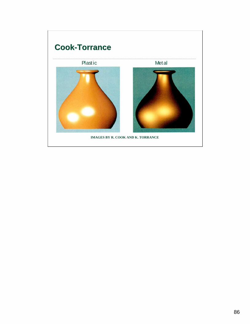
CookCook--TorranceTorrance
Plastic Metal
IMAGES BY R. COOK AND K. TORRANCE
87
CookCook--Torrance Compared to Torrance Compared to Normalized BlinnNormalized Blinn--PhongPhong
• Shadowing, masking modeled more explicitly
• Significantly more expensive to evaluate
• Normalized Blinn-Phong probably a better fit for game rendering
We will use the normalized version of Blinn-Phong as a basis of comparison with other BRDFs.

88
BanksBanks
• Anisotropic version of Blinn-Phong– Surface model composed of threads
– Uses projection of light vector onto plane perpendicular to tangent instead of surface normal
N
T
ωiN’
This is the first anisotropic shader we will discuss. Aside from the new normal vector, this is almost exactly the same as Blinn-Phong. One more difference is that when the light is not in the hemisphere about the original surface normal, the lighting is set to 0 (“self-shadowing” term). This is the only effect the surface normal has on this model.

89
Banks Compared to Normalized Banks Compared to Normalized BlinnBlinn--PhongPhong
• Useful extension of normalized Blinn-Phong– Similar evaluation cost and parameters
• A good fit for modeling certain kinds of anisotropic materials composed of grooves, fibers, etc.– Doesn’t give control over highlight shape, so not
for general anisotropic materials

90
Ward Ward -- IsotropicIsotropic
• Well normalized, meaningful parameters, reciprocal, energy-conserving
• No modeling of
– Shadowing and masking effects
– Body / surface reflectance tradeoff at glancing angles
( ) ( )ei
m
Fd
eir
h
eRm
fθθππ
ωω
θ
coscos0
41ρ,
2tan-
2
⎭⎬⎫
⎩⎨⎧
+=
This is essentially a microfacet model, although it is not explicitly derived from microfacet theory. It uses a modified Beckmann NDF, but no explicit Fresnel or masking / shadowing. It is well normalized however. Note that this version includes corrections that were discovered since the Ward model was first published in 1992. It is physically plausible and has meaningful parameters. Note that the two physical effects that it does not model tend to counteract each other.
91
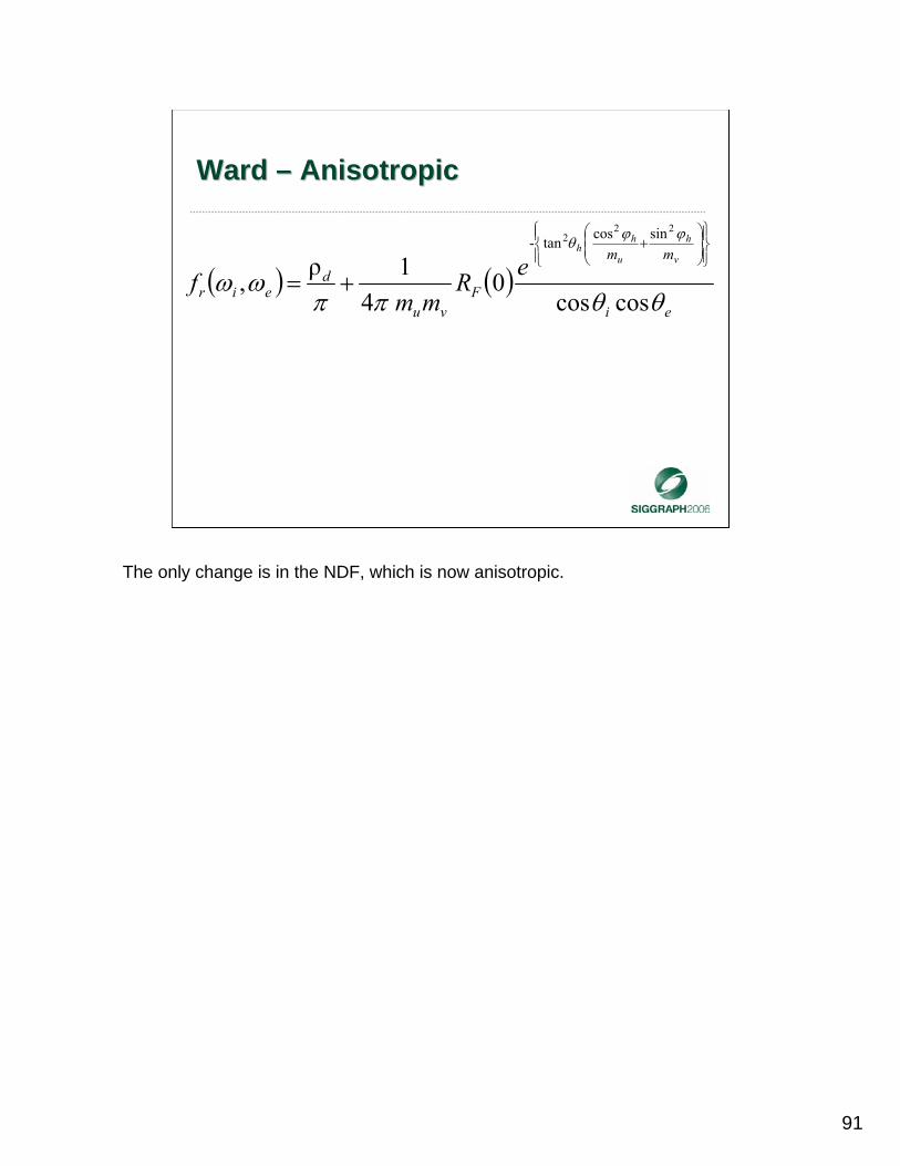
Ward Ward –– AnisotropicAnisotropic
( ) ( )ei
mm
Fvu
deir
v
h
u
hh
eRmm
fθθππ
ωω
ϕϕθ
coscos0
41ρ,
222 sincostan-
⎪⎭
⎪⎬⎫
⎪⎩
⎪⎨⎧
⎟⎟⎠
⎞⎜⎜⎝
⎛+
+=
The only change is in the NDF, which is now anisotropic.
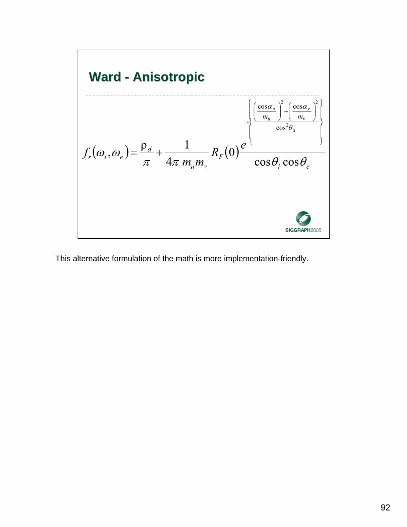
92
Ward Ward -- AnisotropicAnisotropic
( ) ( )ei
mm
Fvu
deir
v
v
u
u
eRmm
fθθππ
ωω
θ
αα
coscos0
41ρ,
h2
22
cos
coscos
-
⎪⎪
⎭
⎪⎪
⎬
⎫
⎪⎪
⎩
⎪⎪
⎨
⎧⎟⎟⎠
⎞⎜⎜⎝
⎛+⎟⎟
⎠
⎞⎜⎜⎝
⎛
+=
This alternative formulation of the math is more implementation-friendly.

93
Ward Ward -- AnisotropicAnisotropic
IMAGE BY G. WARD
Although it is missing some of the features of the physically-based BRDFs, the images still look quite nice.

94
Isotropic Ward Compared to Isotropic Ward Compared to Normalized BlinnNormalized Blinn--PhongPhong
• Reciprocity, precise normalization– Less important for game rendering
• More expensive to evaluate
• Doesn’t seem like a good trade-off for game rendering

95
Anisotropic Ward Compared to Anisotropic Ward Compared to Normalized BlinnNormalized Blinn--PhongPhong
• Even more expensive to evaluate
• More expressive, can do general anisotropy
• Might be a good fit if precise control of highlight shape important
96
AshikhminAshikhmin--ShirleyShirley
• Designed to handle tradeoff between surface and body reflectance at glancing angles– While being reciprocal, energy conserving and well
normalized
• No attempt to model shadowing and masking
• Tradeoff between diffuse and specular term– One of few BRDFs which don’t use Lambert
Most BRDFs focus on the specular term and simply use a Lambertian term for diffuse reflectance. Since the Ashikhmin-Shirley BRDF was designed to trade off reflectance between the diffuse and specular terms, a different diffuse term is used.

97
AshikhminAshikhmin--Shirley: Diffuse TermShirley: Diffuse Term
• Trades off reflectance with the specular term at glancing angles
• Without losing reciprocity or energy conservation
( ) ( )( ) ⎟⎟⎠
⎞⎜⎜⎝
⎛⎟⎠⎞
⎜⎝⎛ −−⎟
⎟⎠
⎞⎜⎜⎝
⎛⎟⎠⎞
⎜⎝⎛ −−−=
55
2cos11
2cos1101
2328ρ, ei
Fd
eir Rfd
θθπ
ωω
98
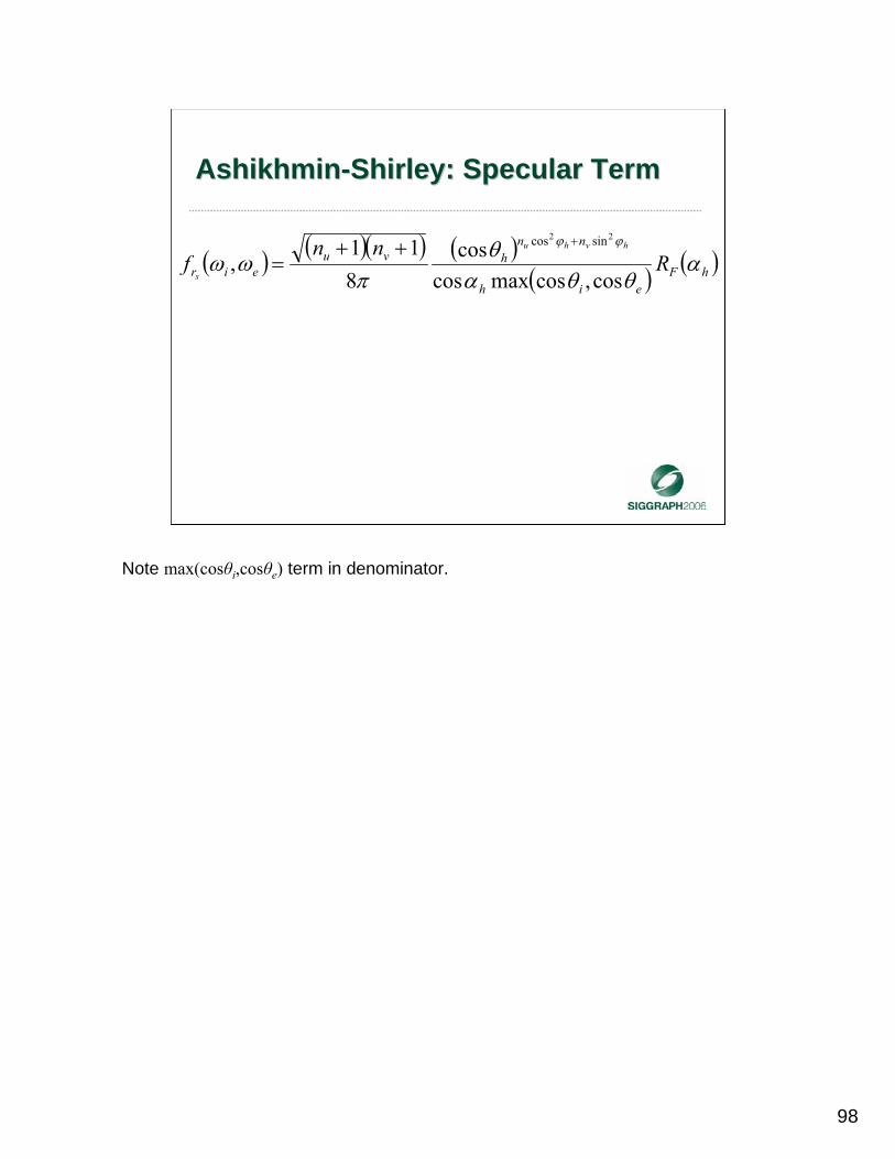
AshikhminAshikhmin--Shirley: Specular TermShirley: Specular Term
( ) ( )( ) ( )( ) ( )hF
eih
nnhvu
eir Rnn
fhvhu
sα
θθαθ
πωω
ϕϕ
cos,cosmaxcoscos
811
,22 sincos +++
=
Note max(cosθi,cosθe) term in denominator.
99
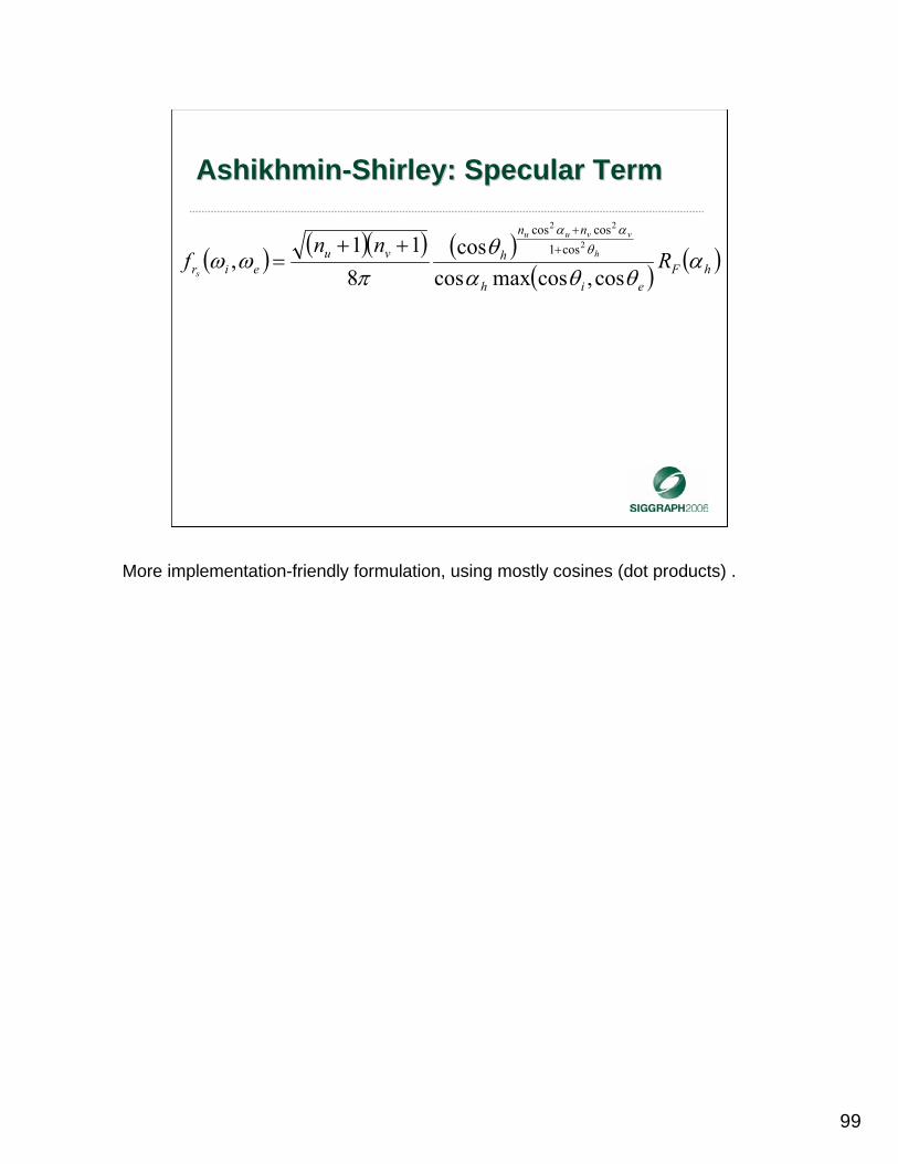
AshikhminAshikhmin--Shirley: Specular TermShirley: Specular Term
( ) ( )( ) ( )( ) ( )hF
eih
nn
hvueir R
nnf h
vvuu
sα
θθαθ
πωω θ
αα
cos,cosmaxcoscos
811
,2
22
cos1coscos
++
++=
More implementation-friendly formulation, using mostly cosines (dot products) .

100
AshikhminAshikhmin--ShirleyShirley
IMAGE BY M. ASHIKHMIN AND P. SHIRLEY
Here we can see how the Ashikhmin-Shirley BRDF allows for controllability of the anisotropy and tightness of the highlight.

101
AshikhminAshikhmin--ShirleyShirley
IMAGE BY M. ASHIKHMIN AND P. SHIRLEY
Here we can see how it models the tradeoff between surface and body reflectance at glancing angles.

102
AshikhminAshikhmin--Shirley Compared to Shirley Compared to Normalized BlinnNormalized Blinn--PhongPhong
• Reciprocity, precise normalization– Less important for game rendering
• Significantly more expressive– General anisotropy (control of highlight shape)
– Correct body-surface reflectance tradeoff
• Expensive to evaluate– Simplified versions worth exploring for games
This BRDF is not currently used much for games, but it is definitely worth taking a closer look at. It has several good properties and it can be modified to be cheaper to evaluate.
103
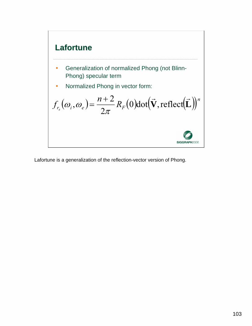
LafortuneLafortune
• Generalization of normalized Phong (not Blinn-Phong) specular term
• Normalized Phong in vector form:
( ) ( ) ( )( )nFeir Rnf
s
reflect,dot0
22, LV
rr
πωω +
=
Lafortune is a generalization of the reflection-vector version of Phong.

104
LafortuneLafortune
• In local frame, reflection operator is just multiplying x and y components by -1:
( ) ( ) ( ) ( ) ( )( )zzyyxxFeir Rnfs
LVLVLV 11102
2, +−+−+
=π
ωω
This requires that the light and view direction are in the local frame of the surface (which the BRDF definition assumes anyway).

105
LafortuneLafortune
• Generalize to one spectral (RGB) constant Kj and four scalar constants (Cxj, Cyj, Czj, nj) per term, add several terms (lobes):
( ) ( )∑ ++=j
nzzjzyyjyxxjxjeir
j
sCCCKf , LVLVLVωω
By taking the (-1. -1, 1) that the components were multiplied by as general coefficients, as well as the power term, and generalizing the Fresnel reflectance into a general spectral coefficient, we get a generalized Phong lobe. The Lafortune BRDF is formed by adding several such lobes.

106
LafortuneLafortune
• Phong:
• Lambertian:
• Non-Lambertian diffuse:
• Off-specular reflection:
• Retro-reflection:
• Anisotropy:
Cx > 0, Cy > 0, Cz > 0
K = RF(0), -Cx = -Cy = Cz = ((n+2)/2π)1/n
K = ρd/π, n = 0
K = ρd , Cx = Cy = 0, Cz = (n+2)/2π
Cz < -Cx = -Cy
Cx ≠ Cy
Besides the standard Phong cosine lobe, this can handle many other cases. The non-Lambertian diffuse given here decreases with increasing angle of incidence, this helps to model the surface / body reflectance trade-off with glancing angles.

107
LafortuneLafortune
IMAGE BY D. MCALLISTER, A. LASTRA AND W. HEIDRICH

108
Lafortune Compared to Normalized Lafortune Compared to Normalized BlinnBlinn--PhongPhong
• Very expressive– Control scattering direction, anisotropy
• Is a (generalized) reflection-vector BRDF
• Several lobes required for most materials– More expensive evaluation, much more input data
• Parameters much less intuitive
• Probably not a good fit for games
The fact that the evaluation uses a lot of data is actually more of a concern than a lot of computation – memory access is constantly growing in cost compared to computation. The parameters could be automatically fitted to some other model with more intuitive parameters, or perhaps even to measured data. However, overall the disadvantages for game rendering seem to outweigh the advantages.
109
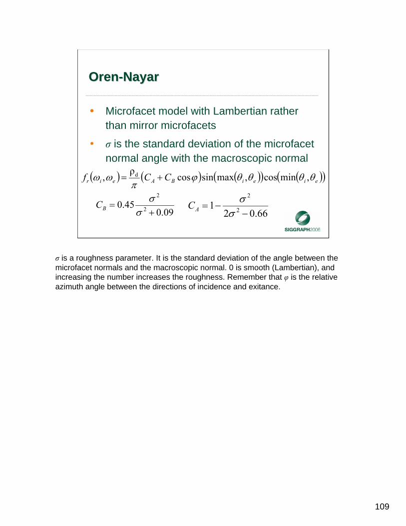
OrenOren--NayarNayar
• Microfacet model with Lambertian rather than mirror microfacets
• σ is the standard deviation of the microfacet normal angle with the macroscopic normal
( ) ( ) ( )( ) ( )( )eieiBAeir CCf θθθθϕπ
ωω ,mincos,maxsincosρ, d +=
66.021 2
2
−−=
σσ
AC09.0
45.0 2
2
+=
σσ
BC
σ is a roughness parameter. It is the standard deviation of the angle between the microfacet normals and the macroscopic normal. 0 is smooth (Lambertian), and increasing the number increases the roughness. Remember that φ is the relative azimuth angle between the directions of incidence and exitance.

110
OrenOren--NayarNayar
• Normalized, reciprocal, physically based
IMAGE BY M. OREN AND S. NAYAR

111
OrenOren--NayarNayar Compared to Normalized Compared to Normalized BlinnBlinn--PhongPhong
• Only models diffuse materials, but models them more realistically and expressively– Added roughness control
• Evaluation cost is reasonable
• Definitely worth looking at for game use– For certain classes of materials

112
IMAGE BY A. NGAN, F. DURAND & W. MATUSIK
Fitting to Measured MaterialsFitting to Measured Materials
We close this discussion of common analytical BRDFs with two charts from recent research comparing the accuracy to which various models fit measured BRDFs. The first chart is sorted on the error of the Blinn-Phong BRDF,

113
IMAGE BY A. NGAN, F. DURAND & W. MATUSIK
Fitting to Measured MaterialsFitting to Measured Materials
And the second is sorted on the error of the Ashikhmin-Shirley BRDF. From these charts we can see that the Ashikhmin-Shirley and Cook-Torrance BRDFs are a good fit to measured BRDFs, while Blinn-Phong, Ward and Lafortune are less accurate but still reasonably close.

1
Analytical BRDFsAnalytical BRDFs
• Common Models (Naty)
• Implementation and Performance (Dan)
• Production Issues (Dan)
Now we shall discuss implementation and performance issues for these models.

2
ImplementationImplementation
• Real time graphics based on rasterization
• Vertices are transformed to make triangles (Vertex Shading)
• Triangles are rasterized into raster triangles (optional Geometry Shading)
• Pixels are shaded and placed into render target (Pixel Shading)
3
Implementing a BRDF Implementing a BRDF
• This means writing GPU shader code
• Can write a program for Vertex, Geometry, or Pixel shader which will evaluate our BRDF
• Most often, evaluation is done at pixel level
Evaluation of BRDFs at vertex level was common several years ago, but with current GPU hardware pixel-level evaluation is almost universal.

4
Data needed for the BRDFData needed for the BRDF
• At each pixel rendered, need– The BRDF parameters
• Reflectance parameters (ρd, RF(0))
• Surface smoothness parameters (n, m, σ)
– For each light: direction ωl, intensity il(dl) at pixel
– Direction from pixel to camera ωe
– If ωi, ωe not in local frame then axes (N, T, B)• Isotropic BRDFs only need N
There is various data needed to evaluate an analytical BRDF. Note that the light intensity is a spectral quantity, which in practical terms means that R, G and B channels are specified. The BRDF model is evaluated in the local frame, so either the incident and exitant directions need to be given in the local frame, or else the axes of the local frame need to be given (in whatever space the direction vectors are specified) so they can be transformed into local space. A full frame is not required unless the BRDF is anisotropic – isotropic BRDFs need only N.

5
Light IntensityLight Intensity
• The computation of il(dl) at each pixel may be very simple or quite complicated depending on the light type– For a directional light, simply a constant
– For an überlight, requires significant computation
– Shadows add even more complexity
• We ignore these complexities for now– Outside the scope of BRDF computation
We will ignore the complexities of computing the attenuated light intensity to a large extent in the following discussion (we will touch upon them in the discussion of shader combinatorial issues later).
6
Spaces / Coordinate SystemsSpaces / Coordinate Systems
• There are various spaces, or coordinate systems, in which directions are specified– Camera space, screen space
– World space
– Object or pose space (rigid or skinned objects)
– Unperturbed tangent space (vertex local frame)
– Perturbed tangent space (pixel local frame)
The directions of incidence and exitance are ultimately needed in the local frame or coordinate system. There are various possible spaces or coordinate systems used in game renderers.Vertex positions are transformed to camera space and screen space to be rendered, but reflectance computations are rarely performed there (deferred rendering systems are an exception).World space is where the object transforms, the camera and light locations are initially specified, reflectance computations are rarely performed there for point lights (although environment map lighting is often performed in world space since that is where the environment map is defined).Object / pose space is where the object vertex positions are initially specified.The normals stored in a normal map (normal texture) are most commonly specified in a per-vertex tangent space. This space is closely related to the texture mapping coordinates used for the normal map. For this reason most game models have N, Tand B vectors stored at the vertices (specified in object space). Often only two are stored and the third derived from them.Finally, the normal map itself (and a twist map if such is used) perturb the local frame (in which the BRDF is defined) at each pixel, defining yet another space.Although the BRDF is defined in the perturbed tangent space, it may be computed in any space if all vectors have been transformed to that space.

7
Spaces for Analytical BRDF Spaces for Analytical BRDF Computation with Point LightsComputation with Point Lights
• One common scheme:– ωi, ωe computed at vertices, transformed into
vertex tangent space, interpolated over triangle
– Per pixel, BRDF computed in unperturbed tangent space with:
• Interpolated ωi, ωe
• N read from normal map
• Optionally T read from twist map
There are various possible schemes for computing analytical BRDFs with point lights, in terms of the spaces in which the computations are performed and where transformations between spaces occur. We will discuss two of the most common schemes.

8
Spaces for Analytical BRDF Spaces for Analytical BRDF Computation with Point LightsComputation with Point Lights
• Another common scheme:– World space position, tangent space axes
interpolated from vertices over triangle
– Per pixel, BRDF computed in world space with:• ωi, ωe computed per pixel
• N read from normal map and transformed to world space
• Optionally T from twist map transformed to world space
Of these two schemes, the first uses less interpolated data if only one light computed, but more if several lights are computed. The two schemes also represent a tradeoff of pixel shader vs. vertex shader computations. There may also be a quality difference between the two. The first scheme tends to show artifacts due to low vertex tessellation.The second scheme is theoretically more correct, but paradoxically this can lead to it producing more artifacts in some cases, since models often simulate curved surfaces via triangles, and the second scheme may reveal this “pretense” due to its greater accuracy. In the end, which of these schemes is preferable depends on the specifics of the game environment and models, as well as the characteristics of the platform used.

9
InterpolatorsInterpolators
• Computing or storing a value on a vertex and interpolating it over the triangle can often save pixel processing
• However, interpolation is strictly linear, which may cause problems with– Directions
– Nonlinear BRDF parameters
• Higher vertex counts help
Interpolating directions is quite common. This causes normalized (length 1) vectors to become non-normalized, but this is easily remedied in the pixel shader by re-normalizing them. Second-order discontinuities may sometimes cause more subtle artifacts. Values on which the resulting color depends in a highly non-linear fashion may also introduce problems when linearly interpolated. If the scene is highly tessellated, then these issues are much reduced, but this may not always be possible due to performance limitations of the vertex processing.

10
ShiftShift--Variant BRDFsVariant BRDFs
• Besides normal / tangent perturbation, BRDF parameters may also vary over the surface
• ρd is most commonly stored in textures, sometimes modulated by vertex values
• RF(0) usually stored in textures as a scalar (gloss map) to save storage
• Both modulated by material constants
Real-world surfaces exhibit a lot of fine-grained variation. Normal and (less commonly) twist mapping help game artists model this variation, but this is not enough – usually the parameters of the BRDF need to be varied as well. This variance is often achieved by storing these parameters in textures. They are sometimes stored on vertices, or vertex and texture values can be combined to reduce visual repetition from texture tiling. Combining these also with material constants facilitates reusing the same textures over different objects. This can also save storage, for example in the common case where a spectral (RGB) value for specular color (RF(0)) is arrived at by multiplying a scalar value stored in a texture (gloss map) with an RGB material constant.
11
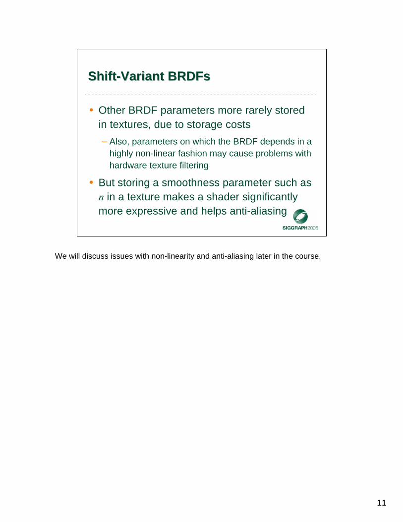
ShiftShift--Variant BRDFsVariant BRDFs
• Other BRDF parameters more rarely stored in textures, due to storage costs– Also, parameters on which the BRDF depends in a
highly non-linear fashion may cause problems with hardware texture filtering
• But storing a smoothness parameter such as n in a texture makes a shader significantly more expressive and helps anti-aliasing
We will discuss issues with non-linearity and anti-aliasing later in the course.

12
Translating BRDF Math to ShadersTranslating BRDF Math to Shaders
• The three-component dot-product is the workhorse of shader BRDF computation– Hardware performs it quickly, can be used to
compute cosines between normalized vectors
• Vector normalization and sqrt used to be expensive, but are becoming quite cheap
• pow, sin, tan, exp etc. more expensive
• Texture reads somewhat expensive
Texture reads are particularly notable for their high latency, so multiple dependent texture reads may have a particularly adverse effect on performance.

13
Translating BRDF Math to ShadersTranslating BRDF Math to Shaders
• We use a different notation for shader code:– L instead of ωi
– V instead of ωe
– H instead of ωh
– R instead of ωri
Since shader languages do not support Greek letters in variable names, we will use a slightly different notation when writing shader code.

14
Translating BRDF Math to ShadersTranslating BRDF Math to Shaders
• Most BRDF sub-expressions translate well:– cos θl becomes saturate(dot(L,N))
– cos θe becomes saturate(dot(V,N))
– cos θh becomes saturate(dot(H,N))
– cos αu becomes saturate(dot(H,T))
– cos αv becomes saturate(dot(H,B))
– cos αr becomes saturate(dot(R,V))
– cos αh becomes saturate(dot(H,V)) or (H,L)
Note that we use θl instead of θi here. This is because when evaluating BRDFs with point lights, ωi is replaced with ωl. The saturate function clamps the result in the range between 0 and 1 – recall that all cosine terms in this course are presumed to be clamped to 0. This clamping operation is free on most modern hardware.As we saw when discussing common analytical BRDFs earlier, almost any BRDF can be reduced to some combination of these sub-expressions.Note that since most of these expressions are dot products with N, T or B, they can be seen also as the Cartesian coordinates of some vector in the local frame.Another thing to note is that in many cases, a vector will appear in dot products the same number of times above and below a division line. In this case the vector does not need to be normalized since its length will cancel out (this happens with H in the Ward and Ashikhmin-Shirley BRDFs).

15
Implementing BlinnImplementing Blinn--PhongPhong
• The Blinn-Phong BRDF:
• The game point light reflection equation:
( ) ( )( )nhFd
eir Rnf θππ
ωω cos08
4ρ, ++=
( ) ( ) lelrlle fdiL θωωπ cos,=
We will use Blinn-Phong as an example for implementing an analytical BRDF for rendering with point lights.First we convert the normalized form of the Blinn-Phong BRDF into the form of the game point light reflection equation.

16
Implementing BlinnImplementing Blinn--PhongPhong
• Simplified:
( ) ( )( ) ln
hFdlle RndiL θθ coscos08
4ρ ⎟⎠⎞
⎜⎝⎛ +
+=
( ) ( )( ) ln
hSdlle nKdiL θθ coscosρ +=
This can be further simplified in two ways: the division by 8 can be factored into the reflectance constant in a pre-processing step, resulting in the constant KS. Also, since this shader will almost always be used with quite large values of n, n+4 can be approximated as n.
17
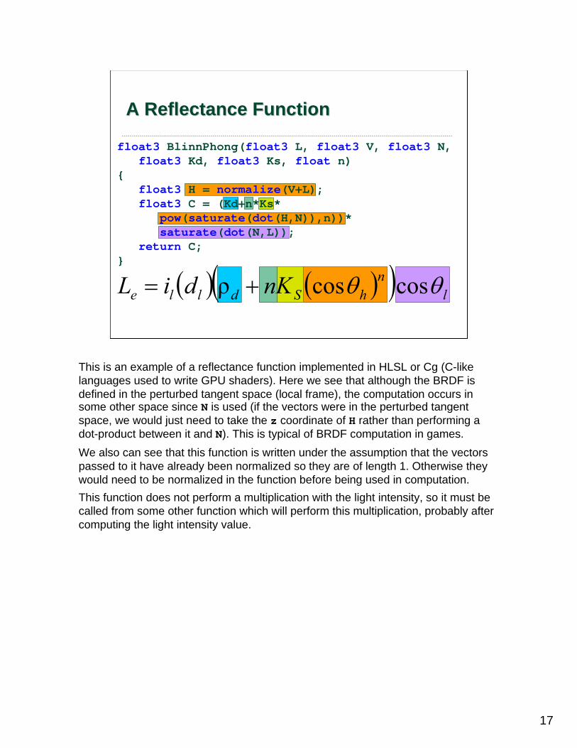
float3 BlinnPhong(float3 L, float3 V, float3 N,float3 Kd, float3 Ks, float n)
float3 H = normalize(V+L);float3 C = (Kd+n*Ks*
pow(saturate(dot(H,N)),n))*saturate(dot(N,L));
return C;
A Reflectance FunctionA Reflectance Function
( ) ( )( ) ln
hSdlle nKdiL θθ coscosρ +=
This is an example of a reflectance function implemented in HLSL or Cg (C-like languages used to write GPU shaders). Here we see that although the BRDF is defined in the perturbed tangent space (local frame), the computation occurs in some other space since N is used (if the vectors were in the perturbed tangent space, we would just need to take the z coordinate of H rather than performing a dot-product between it and N). This is typical of BRDF computation in games.We also can see that this function is written under the assumption that the vectors passed to it have already been normalized so they are of length 1. Otherwise they would need to be normalized in the function before being used in computation.This function does not perform a multiplication with the light intensity, so it must be called from some other function which will perform this multiplication, probably after computing the light intensity value.
18
Pixel Shader (ShiftPixel Shader (Shift--Invariant BRDF)Invariant BRDF)
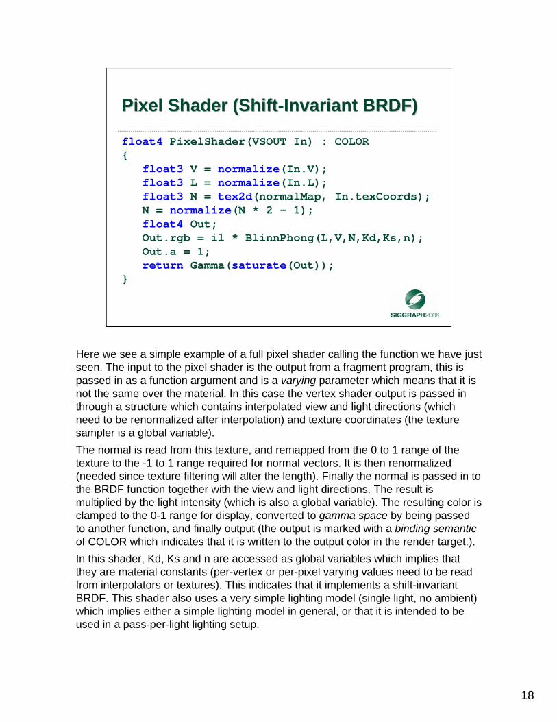
float4 PixelShader(VSOUT In) : COLOR
float3 V = normalize(In.V);float3 L = normalize(In.L);float3 N = tex2d(normalMap, In.texCoords);N = normalize(N * 2 – 1);float4 Out;Out.rgb = il * BlinnPhong(L,V,N,Kd,Ks,n);Out.a = 1;return Gamma(saturate(Out));
Here we see a simple example of a full pixel shader calling the function we have just seen. The input to the pixel shader is the output from a fragment program, this is passed in as a function argument and is a varying parameter which means that it is not the same over the material. In this case the vertex shader output is passed in through a structure which contains interpolated view and light directions (which need to be renormalized after interpolation) and texture coordinates (the texture sampler is a global variable).The normal is read from this texture, and remapped from the 0 to 1 range of the texture to the -1 to 1 range required for normal vectors. It is then renormalized (needed since texture filtering will alter the length). Finally the normal is passed in to the BRDF function together with the view and light directions. The result is multiplied by the light intensity (which is also a global variable). The resulting color is clamped to the 0-1 range for display, converted to gamma space by being passed to another function, and finally output (the output is marked with a binding semanticof COLOR which indicates that it is written to the output color in the render target.).In this shader, Kd, Ks and n are accessed as global variables which implies that they are material constants (per-vertex or per-pixel varying values need to be read from interpolators or textures). This indicates that it implements a shift-invariant BRDF. This shader also uses a very simple lighting model (single light, no ambient) which implies either a simple lighting model in general, or that it is intended to be used in a pass-per-light lighting setup.

19
Gamma SpaceGamma Space
• Gamma is a nonlinear space for radiance– Historically derived from response of CRT displays
– Roughly perceptually uniform
– Useful for storing display radiance values (in 0 to 1 range) in a limited number of bits
– Render targets usually gamma, 8 bits / channel
– Equivalent linear precision would require 11+ bits
– Transfer function roughly: xLinear = xGamma2.2
Gamma is the result of a happy coincidence: the nonlinear response of CRT displays is very close to the inverse of the nonlinear response of the human eye to radiance values. This yields a convenient, perceptually uniform space for storing display radiance values which can be sent directly to the CRT. Even now that CRT displays are no longer in common use, the perceptual uniformity of the space makes it useful. There are various variants of gamma space, but this transfer function has been standardized in Recommendation ITU-R BT.709 (the function shown is in fact slightly simplified from the full Rec. 709 transfer function). Recent hardware has the ability to support high-dynamic-range (HDR) render targets. These are usually in linear space, not gamma space so if rendering to them gamma conversion is not needed.

20
Gamma SpaceGamma Space
• Textures authored w. image editing software– So historically have been stored in gamma space
– Gamma space useful for textures containing non-radiance values such as ρd and RF(0)
• For direct display during editing
• For perceptually uniform low-bit-rate (e.g. 8 bpc) storage
• Most GPUs support conversion from gamma to linear on texture read
Although textures are not strictly display images and do not contain display radiance values, they have historically been edited and stored in in gamma space, and this is still useful for certain types of textures. Since most newer hardware can usually be set up to perform conversion of texture values from gamma to linear on read, this does not often need to be performed in the shader.

21
Gamma ConversionGamma Conversion
• Square-root is cheaper than a power function on most GPUs
• Not exactly transfer function, but close enough
float4 Gamma(float4 linear)
return sqrt(linear);
Some hardware also has functionality to automatically convert from linear to gamma on writing to the render target – in this case gamma conversion on output does not need to be performed in the pixel shader either. In our example, gamma conversion is performed in the pixel shader.
22
Effect FileEffect File
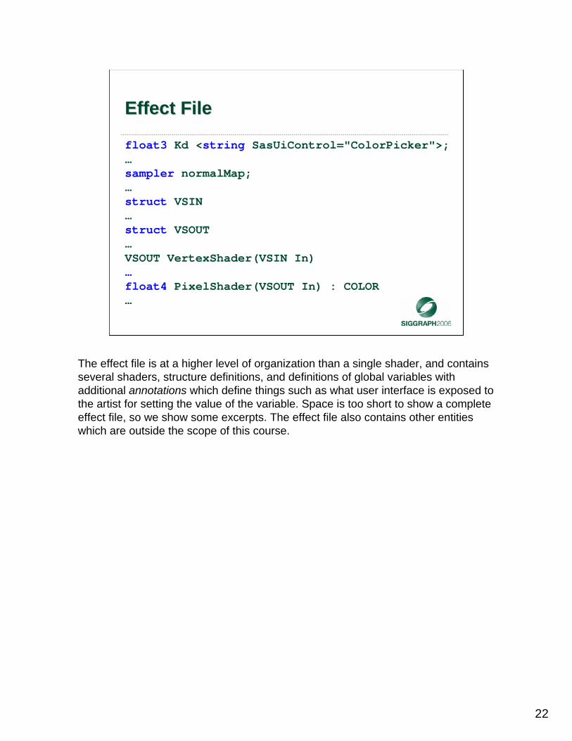
float3 Kd <string SasUiControl="ColorPicker">;…sampler normalMap;…struct VSIN…struct VSOUT…VSOUT VertexShader(VSIN In)…float4 PixelShader(VSOUT In) : COLOR…
The effect file is at a higher level of organization than a single shader, and contains several shaders, structure definitions, and definitions of global variables with additional annotations which define things such as what user interface is exposed to the artist for setting the value of the variable. Space is too short to show a complete effect file, so we show some excerpts. The effect file also contains other entities which are outside the scope of this course.
23
Pixel Shader (ShiftPixel Shader (Shift--Variant BRDF)Variant BRDF)
float4 PixelShader(VSOUT In) : COLOR
…float4 spec = tex2d(specMap, In.texCoords);float n = spec.w;float3 Ks = spec.rgb;float3 Kd = tex2d(diffMap, In.texCoords);float4 Out;Out.rgb = il * BlinnPhong(L,V,N,Kd,Ks,n);Out.a = 1;return Gamma(saturate(Out));
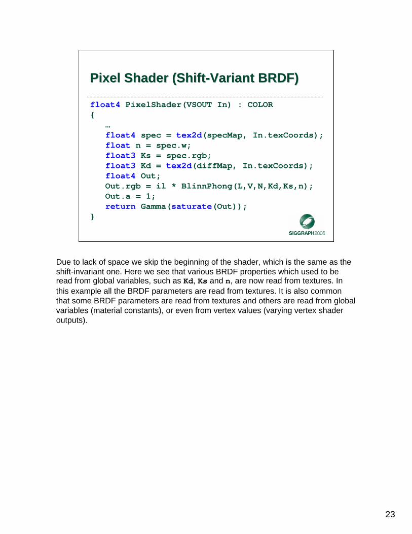
Due to lack of space we skip the beginning of the shader, which is the same as the shift-invariant one. Here we see that various BRDF properties which used to be read from global variables, such as Kd, Ks and n, are now read from textures. In this example all the BRDF parameters are read from textures. It is also common that some BRDF parameters are read from textures and others are read from global variables (material constants), or even from vertex values (varying vertex shader outputs).

24
Anisotropic BRDF with Normal MapAnisotropic BRDF with Normal Map
• Normal map permutes N; T and B are orthogonalized to new N, also vary per-pixel
• Straightforward approach: transform V and Linto per-pixel (perturbed) tangent space– 3 dot products + 3 more per light
• Computation in unperturbed tangent space may be cheaper in some cases– Depends on BRDF and number of lights
It may be tempting to ignore the perturbation in T and B resulting from that of N, but that yields visually poor results. Examining the exact BRDF math and looking at the number of lights will indicate which of the two approaches presented in this slide is cheaper.

25
Anisotropic BRDF with Normal MapAnisotropic BRDF with Normal Map
float4 PixelShader(VSOUT In) : COLOR
…float3 T = normalize(In.T);T = normalize(T – dot(N,T)*N);float3x3 inv = float3x3(T, cross(N,T), N);Lp = mul(L, inv);Vp = mul(V, inv);float4 Out;Out.rgb = il * AnisoBRDF(Lp,Vp,…);Out.a = 1;return Gamma(saturate(Out));
Here we show the straightforward approach for clarity. Gramm-Schmidt is used to create an orthonormal frame after N is perturbed. Since B is created on the fly, it doesn’t need to be passed in from the vertex shader. inv is the inverse of the transform from perturbed to unperturbed tangent space since it is the inverse transpose and it is orthonormal (note that we use pre-multiplication). As in the previous shaders, L and V are interpolated vectors in the unperturbed tangent space, Lp, Vp are in the perturbed tangent space.

26
Anisotropic BRDF with Normal and Anisotropic BRDF with Normal and Twist MapsTwist Maps
• If the twist map is stored as a 3-vector, then we no longer need to orthogonalize– Just read T out of the texture
• However, storage may be a problem
• Naively stored, color + normal + twist will be 12 bytes per texel
• We will discuss texture compression later
12 bytes per texel is quite a lot if we remember the tension between the need for high-resolution textures and the limited storage budget. Usually, hardware texture compression is used, which introduces several new issues.

27
PerformancePerformance
• Different reflectance models, different costs– Computation
– Parameter storage
– Strong hardware trend: computation getting cheaper, storage (relatively) more expensive
• And different benefits– Ease of content creation
– Accuracy, expressiveness
28
Implementation Tradeoffs for Implementation Tradeoffs for Analytical BRDFs with Point LightsAnalytical BRDFs with Point Lights
• Direct Evaluation– Evaluate with ALU instructions in the GPU
• Texture Evaluation– Factor into textures, use as lookup table
• A combination of the 2– Factor some sub-expressions into textures
– Evaluate others with ALU
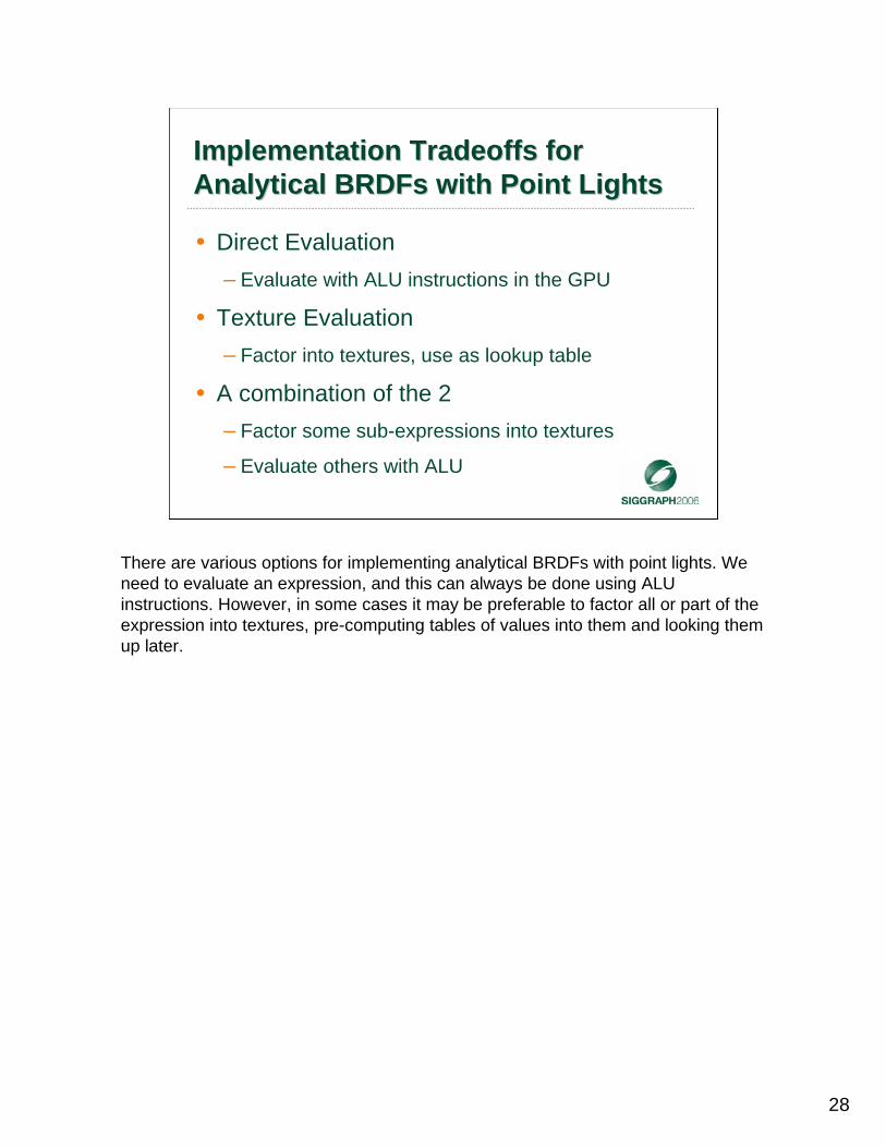
There are various options for implementing analytical BRDFs with point lights. We need to evaluate an expression, and this can always be done using ALU instructions. However, in some cases it may be preferable to factor all or part of the expression into textures, pre-computing tables of values into them and looking them up later.

29
BRDF Costs, ShiftBRDF Costs, Shift--InvariantInvariant
10 + 5 *n0Lafortune Direct
350Cook-Torrance
104Ashikhmin/Shirley factored
400Ashikhmin/Shirley
51Banks Factored
120Banks Direct
21Blinn-Phong factored
70Blinn-Phong Direct
ALU costsTexture costsModel

30
BRDF Costs, ShiftBRDF Costs, Shift--VariantVariant
30 + 5*Lobes2Lafortune Direct
401Cook-Torrance
30 6Ashikhmin/Shirley factored
50 (60)*2Ashikhmin/Shirley
182Banks Factored
251Banks Direct
102Blinn-Phong factored
151Blinn-Phong Direct
ALU costsTexture costsModel
*data cost is similar, so Ashikhmin/Shirley looks attractive, and also Blinn-Phong.

31
Analytical BRDFsAnalytical BRDFs
• Common Models (Naty)
• Implementation and Performance (Dan)
• Production Issues (Dan)
Now, we shall discuss game production issues relating to these reflection models.
32
Production IssuesProduction Issues
• Performance table looks promising, but things are never this simple…
• Each evaluation handles a single point light
• But, game shaders process multiple lights (of different types), shadow maps, other content
• Shaders get long fast! Must multiply cost of BRDF with each light to be evaluated.
Shaders often have to dedicate a fair amount of computation to things other than the reflectance computation, such as shadowing, relief mapping, etc. This must be taken into account when considering the costs of BRDF evaluation.

33
Shader Combinatorics Shader Combinatorics
• Writing a shader for evaluating a BRDF with a particular light set is straightforward
• Writing a shader which can deal with different numbers and types of lights is hard
• In Renderman, lighting and material are distinct shaders – we have no such luxury!
• Solutions: Ubershader, Shader Matrix
Shader combinatorial issues introduce major production problems. Many games have build processes for the shader system which can take hours to compile. A BRDF GPU function ideally will be created in a such a way as to facilitate this.
34
UbershaderUbershader
• Build one monolithic shader with all options
• Problem: size and complexity of the shader
• Flow control may be an issue, but static flow control is getting cheaper
• However, register load is based on the worst-case path, so number of pixels in flight reduced to the worst case

35
Shader MatrixShader Matrix
• Create a Matrix which contains a set of shaders
• For a given set of lights and light types, compile offline a shader for that combination
• Works well – but creates thousands of shaders, which use CPU and memory to process
36
Hybrid TechniquesHybrid Techniques
• Use Ubershader as fallback
• Shader matrix as a cache for commonly used shaders
• Get the best of both worlds
37
Texture ManagementTexture Management
• Expressive shaders use a lot of texture data– Multiple texture reads – lowers performance
– Storage requirements high
• Can often pack data into one texture– Example: store normals as only x and y, pack
power and gloss coefficients in other two channels
– Shader needs to manage unpacking of channels, making authoring more challenging
38
Texture Compression Texture Compression
• Texture formats vary considerably– Bits / pixel, floating / fixed point, compression, etc.
• Hardware compression techniques available– DXT: 4-8 bits per texel – good for color data, poor
for normals, no high dynamic range support
• New Normal Compression in upcoming hardware! Not as efficient as DXT, but gives better results

39
Texture ReparameterizationTexture Reparameterization
• Artists often create large textures with considerable low-detail areas, high percentage of wasted space
• Tools exist to reparameterize texture coordinates based on texture content, can reduce resolution without reducing quality
• Difficult to use with BRDF parameter data– Nonlinear error metrics must be used which are
tailored to the specific BRDF

40
Reflectance Rendering with Point Reflectance Rendering with Point LightsLights
• Analytical BRDFs (Naty & Dan)
• Other Types of BRDFs (Dan)
• Anti-Aliasing and Level-of-Detail (Dan)
Now we shall discuss non-analytical (hand-painted and measured) BRDF models and their implementation and production considerations for rendering with point lights.

41
Other Types of BRDFsOther Types of BRDFs
• Hand-Painted BRDFs
• Measured BRDFs
First, we shall discuss various types of hand-painted BRDFs. Then, we discuss measured BRDFs, with two classes of rendering techniques: factorization and approximation. Finally, we discuss implementation and production issues for the previously mentioned techniques.

42
HandHand--Painted BRDFsPainted BRDFs
• We have discussed how sub-expressions of BRDFs may be put into a texture
• This opens the possibility of having an artist paint the texture to customize the material appearance
• There are several possibilities which offer expressiveness and result in plausible BRDFs

43
NDF MapsNDF Maps
• The normal distribution function (NDF) is the most visually significant component of microfacet-type BRDFs, controlling the highlight shape and size
• Here we see a generalization of Blinn-Phong to a general NDF (KN is a normalization factor)
• The NDF can be painted into a 2D texture– KN computed automatically in tools
( ) ( ) ( )hFNd
eir pRKf ωπ
ωω 0ρ, +=
The value of KN is automatically calculated from the NDF texture in tools to ensure that the BRDF is both reciprocal and energy-conserving. Being able to effectively paint the highlight gives the artist full control over surface smoothness and anisotropy.
44
NDF MapsNDF Maps
• Other BRDF models may use an NDF map, the extended Phong is just an example
• NDFs are high dynamic range by nature– The normalization helps increase range
• NDFs are not spectral quantities– But a colored NDF map can simulate colored
facets with different normal distributions
– Like some fabrics

45
NDF MapsNDF Maps
• For isotropic BRDFS, NDF map is one-dimensional: p(θh)
• Opens possibility of combining with other kinds of hand-painted BRDF information
46
Fresnel RampsFresnel Ramps
• As we have seen earlier, the change in color and magnitude of reflectance with angle of incidence is sometimes complex
• RF(αh) can be stored in a 1D texture or ramp– Computed from material properties, or painted by
an artist to achieve interesting visual effects
– Can be combined with many BRDF models

47
NDF + Fresnel TextureNDF + Fresnel Texture
• A 2D texture mapped by θh on one axis and αh on the other allows hand-painting both arbitrary 1D NDFs and Fresnel functions.
• As well as interactions between the two
• Texture still needs to be processed for normalization

48
Other Types of BRDFsOther Types of BRDFs
• Hand-Painted BRDFs
• Measured BRDFs
Now we will discuss techniques for rendering measured BRDFs.
49
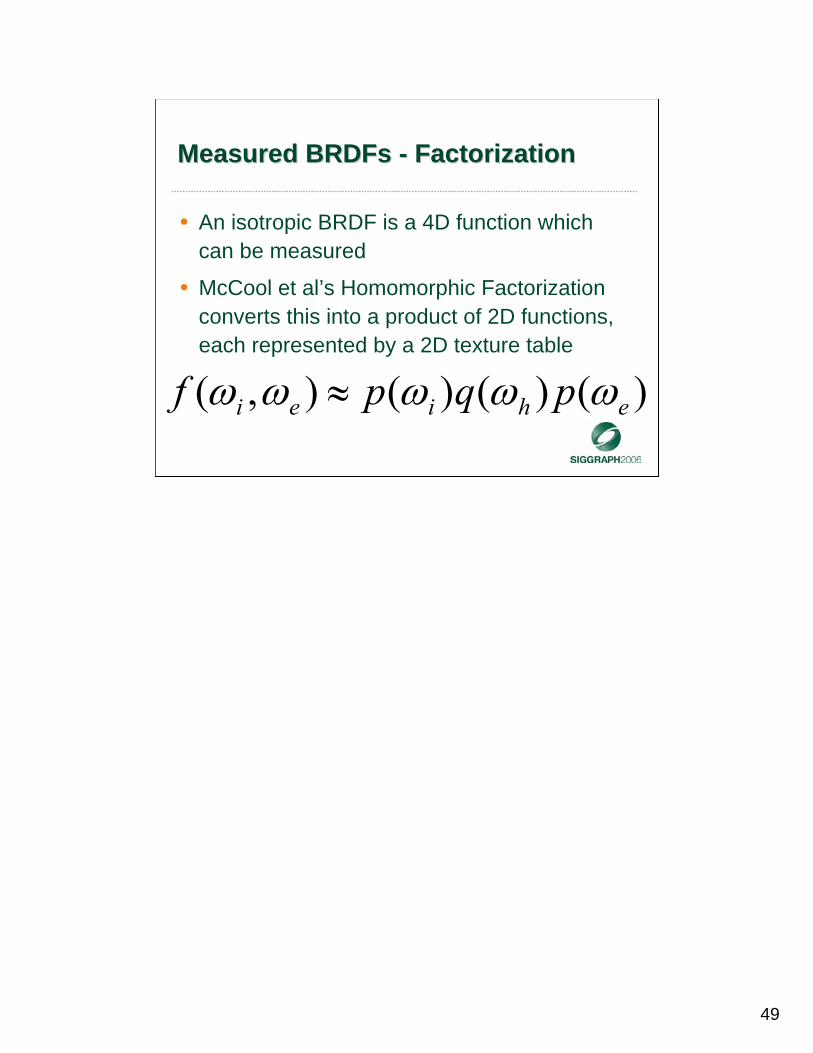
Measured BRDFs Measured BRDFs -- FactorizationFactorization
• An isotropic BRDF is a 4D function which can be measured
• McCool et al’s Homomorphic Factorization converts this into a product of 2D functions, each represented by a 2D texture table
)()()(),( ehiei pqpf ωωωωω ≈

50
Implementation of FactorizationImplementation of Factorization
• In HLSL, Factorization is simple:
float3 BlinnPhong(float3 L, float3 V)
float3 H = normalize(V + L);float3 C = texCUBE(textureP, V) *
texCUBE(textureQ, H) * texCUBE(textureP, L);
return C;
McCools factorization technique is easy to implement, requiring just a few texture lookups. There are various ways to parameterize a texture by a direction, but the most straightforward one is to use the cube-map support in the GPU, which enables using the direction directly to lookup the texture.

51
Measured BRDFs Measured BRDFs –– Approximation Approximation
• [McAllister 2002]: measured BRDFs and fit them to Lafortune model at each texel– Shift-variant Lafortune model
• Could fit any model in this way with the right number of lobes
• But… Data heavy, need texture per lobe
52
Why Measured BRDFs ArenWhy Measured BRDFs Aren’’t Used t Used in Game Renderingin Game Rendering
• Usually only shift-invariant BRDFs supported
• Not easily amenable to artist control
• Existing methods often expensive to render
• New techniques which overcome these drawbacks would be of interest
Artists productivity is very important, so BRDF models which are easy to explain, with parameters that are intuitive to manipulate, are preferred for game development.Research into methods for capturing shift-variant BRDFs of real materials into a format which is efficient to render and easily editable by artists would be valuable for game development.

53
Reflectance Rendering with Point Reflectance Rendering with Point LightsLights
• Analytical BRDFs (Naty & Dan)
• Other Types of BRDFs (Dan)
• Anti-Aliasing and Level-of-Detail (Dan)
Finally in this section, we shall discuss issues relating to anti-aliasing and level-of-detail for reflection models, as rendered with point lights.

54
AntiAnti--Aliasing and LevelAliasing and Level--ofof--DetailDetail
The upper left image is what filtering does to the model, while the lower right image is what it should look like. Notice the hatching patterns caused the linear filtering of BRDF data (in this case Blinn-Phong).

55
AntiAnti--Aliasing and Level of DetailAliasing and Level of Detail
• BRDF models are designed for an infinitely small point
• But pixels cover area, sometimes quite large
• Traditionally, problem mitigated by performing filtering on input data
• Filtering input data for a BRDF isn’t generally meaningful
56
Sampling Woes (Aliasing)Sampling Woes (Aliasing)
• Problem 1: Sample points aren’t stable –small changes in the reading of a sample point can result in drastic rendering differences
• Problem 2: MIP/Linear filtering changes the BRDF. A BRDF composed of a large number of smaller BRDFs is a lot more complex then the average of the input values

57
Pixel Level EvaluationPixel Level Evaluation
The pixel shader will be evaluated at each one of these points.
58
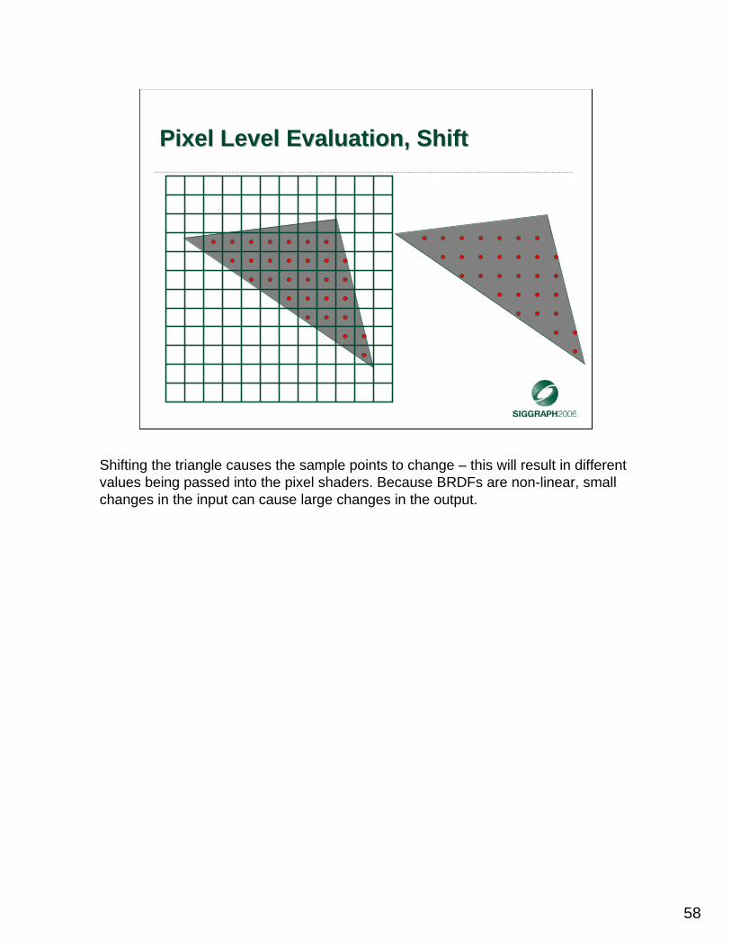
Pixel Level Evaluation, ShiftPixel Level Evaluation, Shift
Shifting the triangle causes the sample points to change – this will result in different values being passed into the pixel shaders. Because BRDFs are non-linear, small changes in the input can cause large changes in the output.

59
What Does a Sample Point Mean?What Does a Sample Point Mean?
What happens What happens when this pixel when this pixel is evaluated? is evaluated?
60
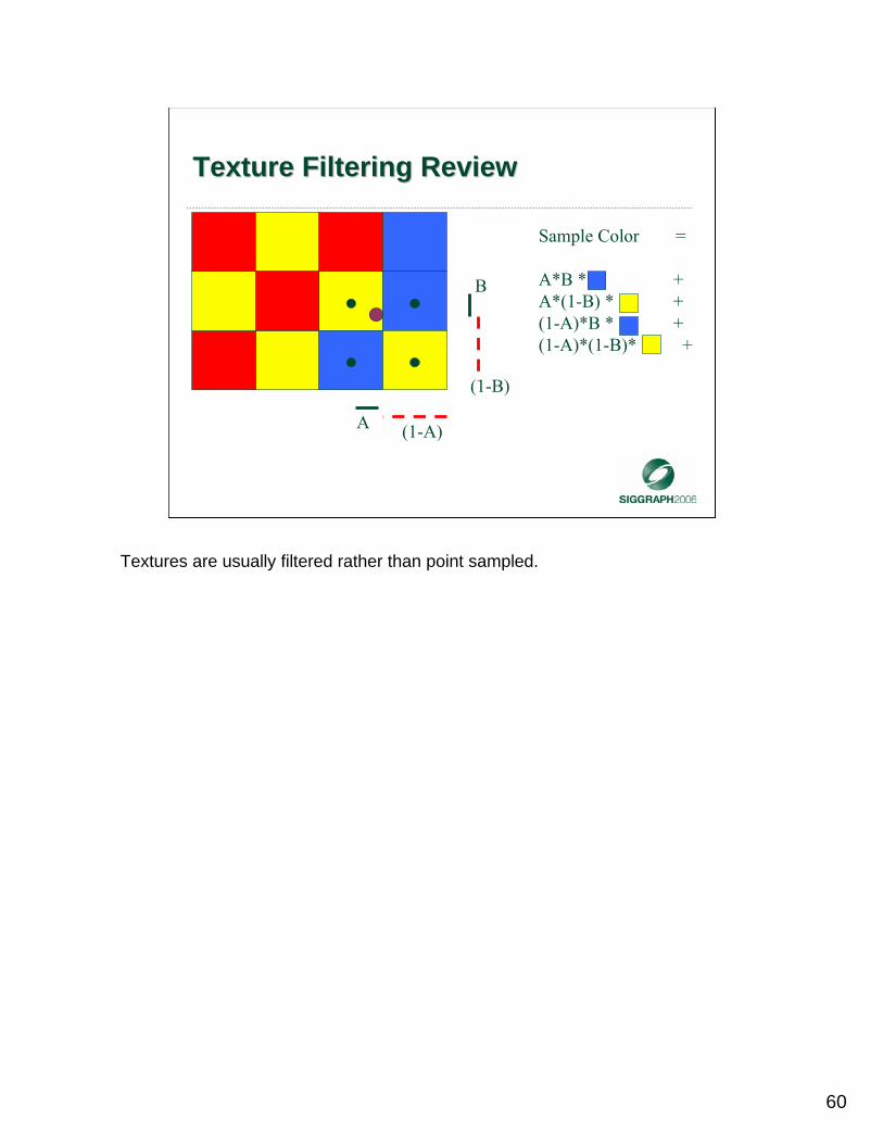
Texture Filtering ReviewTexture Filtering Review
A (1-A)
B
(1-B)
Sample Color =
A*B * +A*(1-B) * +(1-A)*B * +(1-A)*(1-B)* +
Textures are usually filtered rather than point sampled.

61
Problem 1: Texture SamplingProblem 1: Texture Sampling
The color of this pixel changes drastically as the sample points move across the texture. By averaging over disparate normals, we end up with an intermediate vector which aligns to the blue direction vector. When this happens, the pixel may suddenly illuminate because of the tight lobe of this BRDF. Thus, here is a situation where a pixel goes from black to white to black all while the texture moves only 1 pixel. This is an kind of spatial aliasing, often referred to as shimmering.

62
Problem 2: BRDF AveragingProblem 2: BRDF Averaging
If the same triangle is viewed covering a smaller number of pixels (perhaps it is farther away, or the display resolution has been reduced), then the change in filtering of BRDF parameters will have a significant impact on the overall appearance of the BRDF unless the parameters are filtered correctly. This is undesirable – the overall appearance of a surface should not change when it is rendered at lower resolutions.

63
A Common Hack: Level of DetailA Common Hack: Level of DetailM
IP L
evel
Lowering the Lowering the amplitudeamplitudeOf the normal Of the normal displacement, displacement, effectively going to effectively going to a less complex a less complex model with model with distance. This distance. This reduces aliasing, but reduces aliasing, but isnisn’’t accuratet accurate
This is a common trick in many games.

64
Better Hack: Level of DetailBetter Hack: Level of DetailM
IP L
evel
Blinn-Phong n = 32
Blinn-Phong n = 24
Blinn-Phong n = 18
Blinn-Phong n = 12
Blinn-Phong n = 7
Reducing the highReducing the high--frequency content of frequency content of the BRDF by the BRDF by changing BRDF changing BRDF parameters with MIP parameters with MIP level. This still isnlevel. This still isn’’t t accurate, but is accurate, but is better than the better than the previous hack.previous hack.
Decreasing the high-frequency content of the BRDF helps. For example, in the case of Blinn-Phong, decreasing the n parameter by about 30% for each MIP level greatly increases visual quality. This number, however, is just an heuristic, and varies considerably depending on the content.

65
Scale Independent LightingScale Independent Lighting
• Ideally, screen size of an object should not affect its overall appearance
• As screen size decreases– High frequency detail should disappear
– Global effects should stay the same
• This is the reasoning behind MIP mapping
• Avoid drastic changes in image as sample points change
66
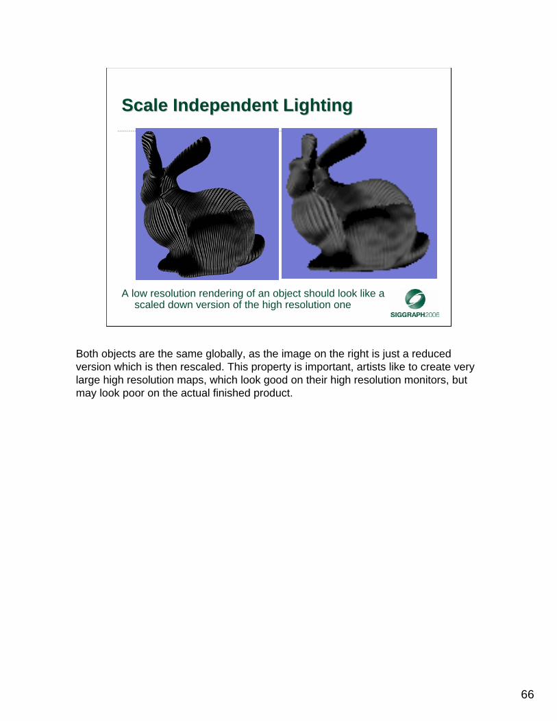
Scale Independent LightingScale Independent Lighting
A low resolution rendering of an object should look like a scaled down version of the high resolution one
Both objects are the same globally, as the image on the right is just a reduced version which is then rescaled. This property is important, artists like to create very large high resolution maps, which look good on their high resolution monitors, but may look poor on the actual finished product.
67
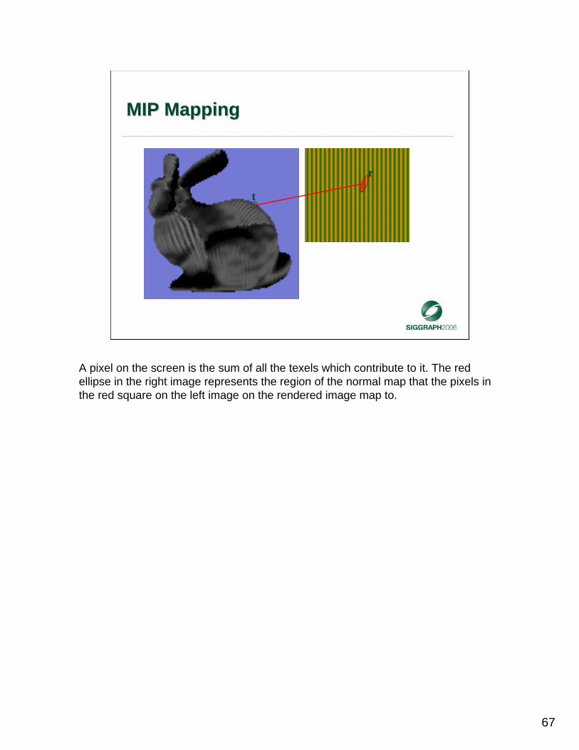
MIP MappingMIP Mapping
r
t
A pixel on the screen is the sum of all the texels which contribute to it. The red ellipse in the right image represents the region of the normal map that the pixels in the red square on the left image on the rendered image map to.
68
MIP mapping for diffuseMIP mapping for diffuse
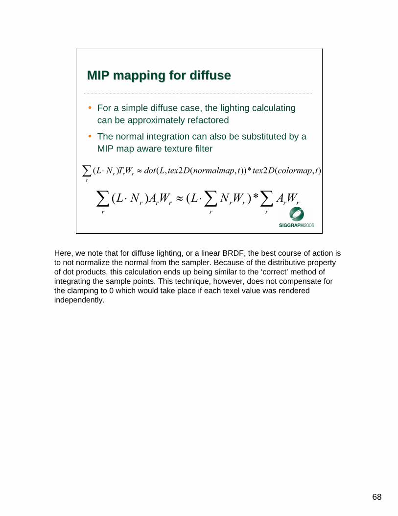
• For a simple diffuse case, the lighting calculating can be approximately refactored
• The normal integration can also be substituted by a MIP map aware texture filter
rr
rr
rrrrr
r WAWNLWANL ∑∑∑ ⋅≈⋅ *)()(
),(2*)),(2,()( tcolormapDtextnormalmapDtexLdotWTNL rrr
r ≈⋅∑
Here, we note that for diffuse lighting, or a linear BRDF, the best course of action is to not normalize the normal from the sampler. Because of the distributive property of dot products, this calculation ends up being similar to the ‘correct’ method of integrating the sample points. This technique, however, does not compensate for the clamping to 0 which would take place if each texel value was rendered independently.

69
Nonlinear BRDFsNonlinear BRDFs
prr
r
prr NWHHNW ∑∑ ⋅≠⋅ )*()(
p
r
prr tnormalmapDtexHHNW )),(2()(∑ ⋅≠⋅
BlinnBlinn--Phong isnPhong isn’’t Lineart Linear
Looking at just the specular component of Blinn-Phong with a normal that varies (the tex2D(r) part), we can see that we cannot use a linear filter. We can think of this as shading on the texels rather than the pixels.
70
SolutionsSolutions
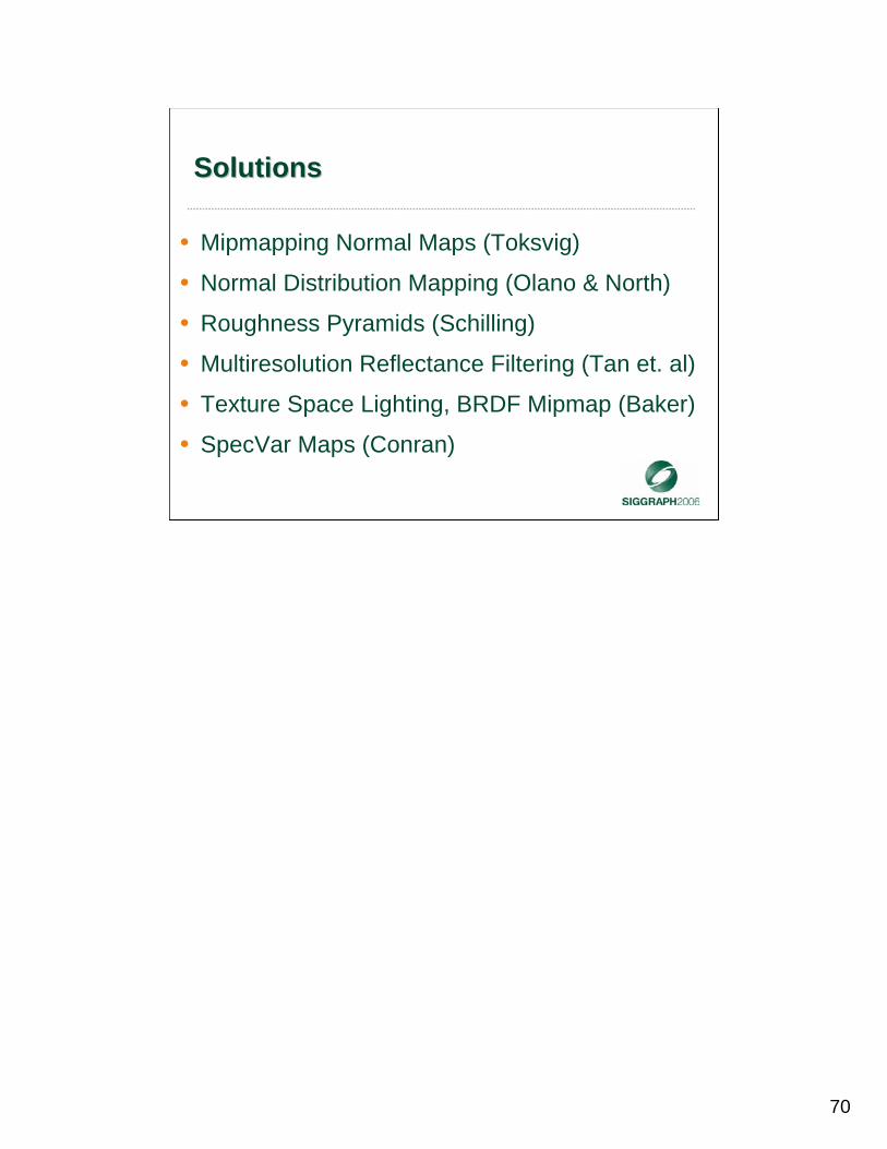
• Mipmapping Normal Maps (Toksvig)
• Normal Distribution Mapping (Olano & North)
• Roughness Pyramids (Schilling)
• Multiresolution Reflectance Filtering (Tan et. al)
• Texture Space Lighting, BRDF Mipmap (Baker)
• SpecVar Maps (Conran)
71
Texture Space LightingTexture Space Lighting
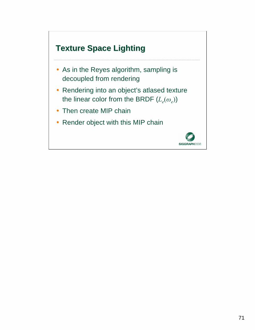
• As in the Reyes algorithm, sampling is decoupled from rendering
• Rendering into an object’s atlased texture the linear color from the BRDF (Le(ωe))
• Then create MIP chain
• Render object with this MIP chain

72
Texture Space LightingTexture Space Lighting
• Triangles rasterized using texture coordinate as screen position
• Left image shows normal sampled at each point
• Right image shows the computed lighting
Here, we see a lit texture and the normal map which generated it. This texture is a mapping of the Stanford bunny. As the model moves through the world, the texture on the right will change as it is illuminated by the lighting environment.

73
Texture Space LightingTexture Space Lighting
• Easy to Implement
• Can be used with any BRDF – Just drop it in and it will work
• Performance problems result - each object is rendered at a locked, often high resolution
• Invisible pixels will be rendered
• Still need a low-resolution substitute

74
Correctly Correctly MipMip--Mapping BRDF Mapping BRDF ParametersParameters
The images in the middle column were rendered using a BRDF-approximating MIP-map. The more we zoom out, the larger the difference between the correct and incorrect approaches. The Stanford bunny is much too shiny when highly minified., because the specular power is not adjusted appropriately.
75
Creating a BRDF MIP ChainCreating a BRDF MIP Chain
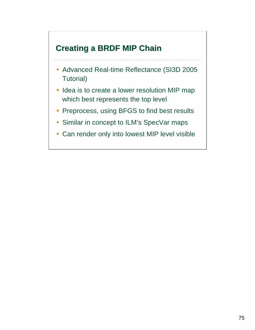
• Advanced Real-time Reflectance (SI3D 2005 Tutorial)
• Idea is to create a lower resolution MIP map which best represents the top level
• Preprocess, using BFGS to find best results
• Similar in concept to ILM’s SpecVar maps
• Can render only into lowest MIP level visible

76
Multiresolution Reflectance MapsMultiresolution Reflectance Maps
• EGSR 2005
• Uses Cook-Torrance BRDF
• Pre-filters so that the Gaussian element of Cook-Torrance can be added by the linear interpolators
• Heavyweight – 250 instructions, 4 textures
• But good results
While the instruction count is high, each additional light is circa 160 instructions for Cook-Torrance (4 lobes at 40 cycles each). The main limitation, however, will probably be the memory requirements, since this takes about 4x the memory of Blinn-Phong. However, it is a one pass technique, unlike texture space lighting.

77
Multiresolution Reflectance MapsMultiresolution Reflectance Maps
IMAGES BY P. TAN, S. LIN, L. QUAN, B. GUO AND H-Y SHUM
The image on the left shows the result of the naive approach, while the center is a reference version. The image on the far right is the multi-resolution reflectance version. Notice the naive approach is much too shiny, just like the Stanford bunny was.


![chap08 reflection.ppt [相容模式]cyy/courses/rendering/14fall/lectures/... · • core/reflection.* • Material = BSDF that combines multiple BRDFs and BTDFs. ((p)chap. 9) •](https://static.fdocuments.us/doc/165x107/5f83c8f0d479922a354a7f50/chap08-c-cyycoursesrendering14falllectures-a-corereflection.jpg)