
10.1.1.54.4570
30
Feature Selection with Neural Networks Philippe LERAY and Patrick GALLINARI LIP6 - Pôle IA Université Paris 6 - boite 169 4, Place Jussieu 75252 Paris cedex 05 France {Philippe.Leray , Patrick.Gallinari}@lip6.fr
-
Upload
seong-gon-kim -
Category
Documents
-
view
213 -
download
1
description
asdfasdf
Transcript of 10.1.1.54.4570

Feature Selection with Neural Networks
Philippe LERAY and Patrick GALLINARI
LIP6 - Pôle IA
Université Paris 6 - boite 169
4, Place Jussieu
75252 Paris cedex 05
France
{Philippe.Leray , Patrick.Gallinari}@lip6.fr

Feature Selection with Neural Networks
Philippe LERAY and Patrick GALLINARI
Abstract
Features gathered from the observation of a phenomenon are not all equally
informative: some of them may be noisy, correlated or irrelevant. Feature
selection aims at selecting a feature set that is relevant for a given task. This
problem is complex and remains an important issue in many domains. In the field
of neural networks, feature selection has been studied for the last ten years and
classical as well as original methods have been employed. This paper is a review
of neural network approaches to feature selection. We first briefly introduce
baseline statistical methods used in regression and classification. We then
describe families of methods which have been developed specifically for neural
networks. Representative methods are then compared on different test problems.
Keywords
Feature Selection, Subset selection, Variable Sensitivity, Sequential Search

Sélection de Variables et Réseaux de Neurones
Philippe LERAY et Patrick GALLINARI
Résumé
Les données collectées lors de l'observation d'un phénomène ou mesurées sur un
système physique ne sont pas toutes aussi informatives: certaines variables
peuvent correspondre à du bruit, être peu significatives, corrélées ou non
pertinentes pour la tâche à réaliser. La sélection de variables est donc un problème
complexe et fait l'objet de recherches dans de nombreuses disciplines. Dans le
domaine des réseaux de neurones, la sélection de variables est étudiée depuis une
dizaine d'années et un certain nombre de méthodes, plus ou moins proches des
méthodes classiques, ont émergé. Ce rapport est une revue des approches
connexionnistes pour la sélection de variables. Nous présentons tout d'abord les
différents éléments constituant une méthode de sélection de variables. Nous
évoquons ensuite brièvement les méthodes statistiques utilisées en régression et
en classification. Nous passons enfin en revue les principales méthodes
développées spécialement pour les réseaux de neurones. Plusieurs méthodes
représentatives de sélection de variables sont alors comparées sur différents
problèmes.
Mots Clés
Sélection de Variables, Sélection de Caractéristiques, Pertinence d'une Variable,
Recherche Séquentielle
Feature Selection with Neural Networks - Philippe Leray and Patrick Gallinari 1
Feature Selection with Neural Networks
Philippe LERAY and Patrick GALLINARI
1. Introduction
Learning systems primary source of information is data. For numerical systems
like Neural Networks (NNs), data are usually represented as vectors in a
subspace of Rk whose components - or features - may correspond for example to
measurements performed on a physical system or to information gathered from
the observation of a phenomenon. Usually all features are not equally
informative: some of them may be noisy, meaningless, correlated or irrelevant for
the task. Feature selection aims at selecting a subset of the features which is
relevant for a given problem. It is most often an important issue: the amount of
data to gather or process may be reduced, training may be easier, better estimates
will be obtained when using relevant features in the case of small data sets, more
sophisticated processing methods may be used on smaller dimensional spaces
than on the original measure space, performances may increase when non
relevant information do not interfere, etc.
Feature selection has been the subject of intensive researches in statistics and in
application domains like pattern recognition, process identification, time series
modelling or econometrics. It has recently began to be investigated in the machine
learning community which has developed its own methods. Whatever the domain
is, feature selection remains a difficult problem. Most of the time this is a non
monotonous problem, i.e. the best subset of p variables does not always contain
the best subset of q variables (q < p). Also, the best subset of variables depends
on the model which will be further used to process the data - usually, the two
steps are treated sequentially. Most methods for variable selection rely on
heuristics which perform a limited exploration on the whole set of variable
combinations.
In the field of NNs, feature selection has been studied for the last ten years and
classical as well as original methods have been employed. We discuss here the
problem of feature selection specifically for NNs and review original methods
Feature Selection with Neural Networks - Philippe Leray and Patrick Gallinari 2
which have been developed in this field. We will certainly not be exhaustive since
the literature in the domain is already important, but the main ideas which have
been proposed are described.
We describe in sections 2 and 3 the basic ingredients of feature selection methods
and the notations. We then briefly present, in section 4, statistical methods used
in regression and classification. They will be used as baseline techniques. We
describe, in section 5, families of methods which have been developed
specifically for neural networks and may be easily implemented either for
regression or classification tasks. Representative methods are then compared on
different test problems in section 6.
2. Basic ingredients of feature selection methods.
A feature selection technique typically requires the following ingredients:
• a feature evaluation criterion to compare variable subsets, it will be
used to select one of these subsets,
• a search procedure, to explore a (sub)space of possible variable
combinations,
• a stop criterion or a model selection strategy.
2.1.1 Feature evaluation
Depending on the task (e.g. prediction or classification) and on the model (linear,
logistic, neural networks...), several evaluation criteria, based either on statistical
grounds or heuristics, have been proposed for measuring the importance of a
variable subset. For classification, classical criteria use probabilistic distances or
entropy measures, often replaced in practice by simple interclass distance
measures. For regression, classical candidates are prediction error measures. A
survey of classical statistical methods may be found in (Thomson 1978) for
regression and (McLachlan 1992) for classification.
Some methods rely only on the data for computing relevant variables and do not
take into consideration the model which will then be used for processing these
data after the selection step. They may rely on hypothesis about the data
distribution (parametric methods) or not (non parametric methods). Other
Feature Selection with Neural Networks - Philippe Leray and Patrick Gallinari 3
methods take into account simultaneously the model and the data - this is usually
the case for NN variable selection.
2.1.2 Search
In general, since evaluation criteria are non monotonous, comparison of feature
subsets amounts to a combinatorial problem (there are 2k -1 possible subsets for
k variables), which rapidly becomes computationally unfeasible, even for
moderate input size. Branch and Bound exploration (Narendra and Fukunaga
1977) allows to reduce the search for monotonous criteria, however the
complexity of these procedures is still prohibitive in most cases. Due to these
limitations, most algorithms are based upon heuristic performance measures for
the evaluation and sub-optimal search. Most sub-optimal search methods follow
one of the following sequential search techniques (see e.g. Kittler, 1986) :
• start with an empty set of variables and add variables to the already
selected variable set (forward methods)
• start with the full set of variables and eliminate variables from the
selected variable set (backward methods)
• start with an empty set and alternate forward and backward steps
(stepwise methods). The Plus l - Take away r algorithm is a
generalisation of the basic stepwise method which alternates l
forward selections and r backward deletions.
2.1.3 Subset selection - Stopping criterion
Let be given a feature subset evaluation criterion and a search procedure. Several
methods examine all the subsets provided by the search (e.g. 2k-1 for an
exhaustive search or k for a simple backward search) and select the most relevant
according to the evaluation criterion.
When the empirical distribution of the evaluation measure or of related statistics is
known, tests may be performed for the (ir)relevance hypothesis of an input
variable. Classical sequential selection procedures use a stop criterion: they
examine the variables sequentially and stop as soon as a variable is found
irrelevant according to a statistical test. For classical parametric methods,
distribution characteristics (e.g. estimates of the evaluation measure variance) are
easily derived (see sections 4.1 and 4.2). For non parametric or flexible methods

Feature Selection with Neural Networks - Philippe Leray and Patrick Gallinari 4
like NNs, these distributions are more difficult to obtain. Confidence intervals
which would allow to perform significance testing might be computed via monte
carlo simulations or bootstrapping. This is extremely prohibitive and of no
practical use except for very particular cases (e.g. Baxt and White 1996).
Hypothesis testing is thus seldom used with these models. Many authors use
instead heuristic stop criteria.
A better methodology, whose complexity is still reasonable in most applications,
is to compute for the successive variable subsets provided by the search
algorithm an estimate of the generalization error (or prediction risk) obtained with
this subset. The selected variables will be those giving the best performances.
The generalization error estimate may be computed using a validation set or
cross-validation or algebraic methods although the latter are not easy to obtain
with non linear models. Note that this strategy involves retraining a NN for each
subset.
3. Notations
We will denote ( , )x y ∈ℜ × ℜk g the realization of a random variable pair (X,Y)
with probability distribution P. xi will be the ith component of x and xl the lth
pattern in a given data set D of cardinality N. In the following, we will restrict
ourselves to one hidden layer NNs, the number of input and output units will be
denoted respectively by k and g. The transfer function of the network will be
denoted f. Training will be performed here according to a Mean Squared Error
criterion (MSE) although this is not restrictive. We will consider, in the
following, selection methods for classification and regression tasks.
4. Model independent Feature Selection
We introduce below some methods which perform the selection and the
classification or regression steps sequentially, i.e. which do not take into account
the classification or regression model during selection. These methods are not
NN oriented and are used here for the experimental comparison with NN specific
selection techniques (section 6). The first two are basic statistical techniques
Feature Selection with Neural Networks - Philippe Leray and Patrick Gallinari 5
aimed respectively at regression and classification. These methods are not well
fitted for NNs since the hypothesis they rely on do not correspond to situations
where NNs might be useful. However since most NN specific methods are
heuristics they should be used for a baseline comparison. The third one has been
developed more recently and is a general selection technique which is data
hypothesis free and might be used for any system either for regression or
classification. It is based on a probabilistic dependence measure between two sets
of variables.
4.1 Feature selection for linear regression
We will consider only linear regression, but the approach described below may
be trivially extended for multiple regression. Let x1, x2, ... xk and y be real
variables which will be supposed centered. Let us denote:
f( p)(x) = bi xii=1
p
∑ (4.1.1)
the current approximation of y with p selected variables (the xi are renumbered so
that the p first selected variables correspond to numbers 1 to p). The residualse f yp p( ) ( ) ( )= −x are assumed identically and independently distributed.
Let us denote:
SST yl
l
N
==∑( )2
1
SSRp = f( p)2 (xl )
l =1
N
∑ (4.1.2)
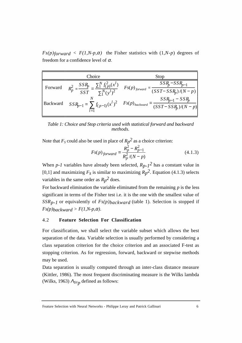
For forward selection, the choice of the pth variable is usually based on Rp2, the
partial correlation coefficient (table 1) between y and regressor f(p), or on an
adjusted coefficient1. This coefficient represents the proportion of y total variance
explained by the regressor f(p). The pth variable to select is the one for which
f(p) maximizes this coefficient. The importance of a new variable is usually
measured via a Fisher test (Thompson, 1978) which compares the models with
p-1 and p variables (Fs(p)forward in table 1). Selection is stopped if
1 The adjusted coefficientRN R p
N ppp22
=∗ −
−is often used instead of Rp
2 .
Feature Selection with Neural Networks - Philippe Leray and Patrick Gallinari 6
Fs(p)forward < F(1,N-p,α) the Fisher statistics with (1,N-p) degrees of
freedom for a confidence level of α.
Choice Stop
Forward Rp2 =
SSRpSST
=f( p)
2 (xl )1N∑
(yl )21N∑
Fs(p) forward =SSRp−SSRp−1
(SST− SSRp) /(N − p)
Backward SSRp−1 = f( p−1)(xl )2
l =1
N
∑ Fs(p)backward =SSRp−1 − SSRp
(SST− SSRp )/(N − p)
Table 1: Choice and Stop criteria used with statistical forward and backwardmethods.
Note that FS could also be used in place of Rp2 as a choice criterion:
Fs pR R
R N pforward
p p
p( )
/( )=
−
−−
21
2
2 (4.1.3)
When p-1 variables have already been selected, Rp-12 has a constant value in
[0,1] and maximizing Fs is similar to maximizing Rp2. Equation (4.1.3) selects
variables in the same order as Rp2 does.
For backward elimination the variable eliminated from the remaining p is the less
significant in terms of the Fisher test i.e. it is the one with the smallest value of
SSRp-1 or equivalently of Fs(p)backward (table 1). Selection is stopped if
Fs(p)backward > F(1,N-p,α).
4.2 Feature Selection For Classification
For classification, we shall select the variable subset which allows the best
separation of the data. Variable selection is usually performed by considering a
class separation criterion for the choice criterion and an associated F-test as
stopping criterion. As for regression, forward, backward or stepwise methods
may be used.
Data separation is usually computed through an inter-class distance measure
(Kittler, 1986). The most frequent discriminating measure is the Wilks lambda(Wilks, 1963) ΛsVp defined as follows:

Feature Selection with Neural Networks - Philippe Leray and Patrick Gallinari 7
Λ S Vp =W
W + B(4.2.1)
where W is the intra-class matrix dispersion corresponding to the selected
variable set SVp, B the corresponding inter-class matrix2 and |M| the determinant
of matrix M. The determinant of a covariance matrix being a measure of the
volume occupied by the data, |W| measures the mean volume of the different
classes and |W+ B| the volume of the whole data set. These quantities are
computed for the selected variables so that a good discriminating powercorresponds to a small value of Λsvp: the different classes are represented by
compact clusters and are well separated. This criterion is well suited in the case of
multinormal distributions with equal covariance for each class, it is meaningless
for e.g. multimodal distributions. This is clearly a very restrictive hypothesis.
With this measurement the statistic Fs, defined below, has a F(g-1,N-g-p+1,α)
distribution (McLachlan 1992):
FS = (N − g − p +1)(g −1)
1− ΛSVp( )ΛSVp
(4.2.2)
We can then use the Wilks lambda both for estimating the discriminating power
of a variable and for stopping the selection in forward, backward (Habbema and
Hermans, 1977) or stepwise methods.
For the comparisons in section 6, we used Stepdisc, a stepwise method based on
(4.2.2) with a 95% confidence level.
4.3 Mutual Information
When data are considered as realization of a random process, probabilistic
information measures may be used in order to compute the relevance of a set of
2 these two quantities are defined as :
W = xl − µ j( )t xl − µ j( )x l ∈class j
∑j =1
g
∑ B = Nj (µ − µ j )t(µ − µ j )j=1
g
∑with g the number of classes, nj the number of samples in class j, µj the mean of
class j and µ the global mean.

Feature Selection with Neural Networks - Philippe Leray and Patrick Gallinari 8
variables with respect to other variables. Mutual information is such a measure
which is defined as:
MI(a,b) = P(a,b) × logP(a,b)
P(a)P(b)
a,b∑ (4.3.1)
where a and b are two variables with probability density P(a) and P(b).
Mutual information is independent from any inversible and differentiable
transformation of the variables. It measures the "uncertainty reduction" on b
when a is known. It is also known as the Kullbak-Leibler distance between the
joint distribution P(a,b) and the marginal distribution product P(a)*P(b).
The method described below does not make use of restrictive assumptions on the
data and is therefore more general and attractive than the ones described in
sections 4.1 and 4.2, especially when these hypothesis do not correspond to the
data processing model, which is usually the case for NNs. It may be used either
for regression or discrimination. On the other hand such non parametric methods
are computationally intensive. The main practical difficulty here is the estimation
of the joint density P(a,b) and of the marginal densities P(a) and P(b). Non
parametric density estimation methods are costly in high dimensions and
necessitate a large amount of data.
The algorithm presented below uses the Shannon entropy (denoted H(.)) to
compute the mutual information MI(a,b) = H(a) + H(b) - H(a,b). It is possible to
use other entropy measures like quadratic or cubic entropies (Kittler, 1986).
Battiti (1994) proposed to use mutual information with a forward selection
algorithm called MIFS (Mutual Information based Feature Selection). P(a,b) is
estimated by Fraser algorithm (Fraser and Swinney, 1986), which recursively
partitions the space using χ2 tests on the data distribution. This algorithm can
only compute the mutual information between two variables. In order to compute
the mutual information between xp and the selected variable set SVp-1 (xp does
not belong to SVp-1), Battiti uses simplifying assumptions. Moreover, the
number of variables to select is fixed before the selection. This algorithms uses
forward search and variable xp is the one which maximises the value :MI(S Vp−1∪ {xp}, y) (4.3.2)
where SVp-1 is the set of p - 1 already selected variables.

Feature Selection with Neural Networks - Philippe Leray and Patrick Gallinari 9
Bonnlander and Weigend (1994) use Epanechnikov kernels for density
estimation (Härdle, 1990) and a Branch&Bound (B&B) algorithm for the search
(Narendra and Fukunaga, 1977). B&B warrants an optimal search if the criterion
used is monotonous and it is less computationally intensive than exhaustive
search. For the search algorithm, one can also consider the suboptimal floating
search techniques proposed by Pudil et al. (1994) which offer a good
compromise between the sequential methods simplicity and the relative
computational cost of the Branch&Bound algorithm.
For the comparisons in section 6, we have used Epanechnikov kernels for
density estimation in (4.3.2), a forward search, and the selection is stopped
when the MI increase falls below a fixed threshold (0.99).
5. Model dependent feature selection for Neural Networks
Model dependent feature selection attempts to perform simultaneously the
selection and the processing of the data: the feature selection process is part of the
training process and features are sought for optimizing a model selection
criterion. This "global optimization" looks more attractive than model-
independent selection where the adequacy of the two steps is up to the user.
However, since the value of the choice criterion depends on the model
parameters, it might be necessary to train the NN with different sets of variables:
some selection procedures alternate between variable selection and retraining of
the model parameters. This forbids the use of sophisticated search strategies
which would be computationally prohibitive.
Some specificities of NNs should also be taken into consideration when deriving
feature selection algorithms:
• NNs are usually non linear models. Since many parametric model-
independent techniques are based on the hypothesis that input-output variables
dependency is linear or that input variables redundancy is well measured by linear
correlation between these variables, such methods are clearly ill fitted for NNs.
• The search space has usually many local minima, and relevance
measures will depend on the minimum the NN will have converged to. These

Feature Selection with Neural Networks - Philippe Leray and Patrick Gallinari 10
measures should be averaged over several runs. For most applications this is
prohibitive and has not been considered here.
• Except for (White 1989) who derives results on the weight distribution
there is no work in the NN community which might be used for hypothesis
testing.
For NN feature selection algorithms, choice criteria are mainly based on heuristic
individual feature evaluation functions. Several of them have been proposed in
the literature, we have made an attempt to classify them according to their
similarity. We will distinguish between:
• zero order methods which use only the network parameter values.
• first order methods which use the first derivatives of network parameters.
• second order methods which use second derivatives of network
parameters.
Most feature evaluation criteria only allow to rank variables at a given time, the
value of the criterion by itself being non informative. However, we will see that
most of these methods work reasonably well.
Feature selection methods with neural networks use mostly backward search
although some forward methods have also been proposed (Moody 1994, Goutte
1997). Several methods use individual evaluation of the features for ranking them
and do not take into consideration their dependencies or their correlations. This
may be problematic for selecting minimal relevant sets of variables. Using the
correlation as a simple dependence measure is not enough since NNs capture non
linear relationships between variables, on the other hand, measuring non linear
dependencies is not trivial. While some authors simply ignore this problem,
others propose to select only one variable at a time and to retrain the network with
the new selected set before evaluating the relevance of remaining variables. This
allows to take into account some of the dependencies the network has discovered
among the variables.
More critical is the difficulty for defining a sound stop criterion or model choice.
Many methods use very crude techniques for stopping the selection, e.g. a
threshold on the choice criterion value, some rank the different subsets using an

Feature Selection with Neural Networks - Philippe Leray and Patrick Gallinari 11
estimation of the generalization error. The latter is the expected error performed
on future data and is defined as:R= r(x, y )p(x, y )∫ dxdy (5.0.1)
where in our case, r(x,y) is the euclidean error between desired and computed
outputs. Estimates can be computed using a validation set, cross-validation or
algebraic approximations of this risk like the Final Prediction Error, (Akaike
1970). Several estimates have been proposed in the statistical (Gustafson and
Hajlmarsson 1995) and NN (Moody 1991, Larsen and Hansen 1994) literature.
For the comparison in section 6, we have used a simple threshold when the
authors gave no indication for the stop criterion and a validation set
approximation of the risk otherwise.
5.1 Zero Order Methods
For linear regression models, the partial correlation coefficient can be expressed
as a simple function of the weights. Although this is not sound for non linear
models, there have been some attempts for using the input weight values in the
computation of variable relevance. This has been observed to be an inefficient
heuristic: weights cannot be easily interpreted in these models.
A more sophisticated heuristic has been proposed by Yacoub and Bennani
(1997), it exploits both the weight value and the network structure of a multilayer
perceptron. They derived the following criterion:
Sw
w
w
wi
ji
jii I
kj
kjj H
k Oj H
=
′
′∈′
′∈∈∈ ∑ ∑∑∑ (5.1.1)
where I, H, O denote respectively the input, hidden and output layer.
For a better understanding of this measure, let us suppose that each hidden and
output unit incoming weight vector has a unitary L1 norm, the above equation
can be written as:
S w wi oj jij Ho O
=∈∈∑∑ (5.1.2)
In (5.1.2), the inner term is the product of the weights from input i to hidden unit
j and from j to output o. The importance of variable i for output o is the sum of
Feature Selection with Neural Networks - Philippe Leray and Patrick Gallinari 12
the absolute values of these products over all the paths -in the NN- from unit i to
unit o. The importance of variable i is then defined as the sum of these values
over all the outputs. Denominators in (5.1.1) operate as normalizing factors, this
is important when using squashing functions, since these functions limit the
effect of weight magnitude. Note that this measure will depend on the magnitude
of the input, the different variables should then be in a similar range. The two
weight layers do have different role in a MLP which is not reflected in (5.1.1),
for example, if the outputs are linear, the normalization should be suppressed in
the inner summation of (5.1.1).
They used a backward search and the NN is retrained after each variable deletion,
the stop criterion is based on the evolution of the performances on a validation
set, elimination is stopped as soon as performances decrease.
5.2 First Order Methods
Several methods propose to evaluate the relevance of a variable by the derivative
of the error or of the output with respect to this variable. These evaluation criteria
are easy to compute, most of them lead to very similar results. These derivatives
measure the local change in the outputs wrt a given input, the other inputs being
fixed. Since these derivatives are not constant like in linear models, they must be
averaged over the training set. For these measures to be fully meaningful, inputs
should be independent and since these measures average local sensitivity values,
the training set should be representative of the input space.
5.2.1 Saliency Based Pruning (SBP)
This backward method (Moody and Utans 1992) uses as evaluation criterion the
variation of the learning error when a variable xi is replaced by its empirical mean
x i (zero here since variables are assumed centered):
Si = MSE− MSE(xi ) (5.2.1)
where MSE xN
f x x x yil
il
kl l
l
N
( ) ( ,..., ,..., )= −=∑1
12
1
Feature Selection with Neural Networks - Philippe Leray and Patrick Gallinari 13
This is a direct measure of the usefulness of the variable for computing the
output. For large values of N, computing Si is costly, and a linear approximation
may be used:
SN
f y
xx xi
l l
il
N
il
il=
−−( )
=∑1
2
1
∂
∂
( )x(5.2.2)
Variables are eliminated in the increasing order of Si.
For each feature set, a NN is trained and an estimate of the generalization error - a
generalization of the Final Prediction Error criterion - is computed. The model
with minimum generalization error is selected.
Changes in MSE is not ambiguous only when inputs are not correlated. Variable
relevance being computed once here, this method does not take into account
possible correlations between variables. Relevance could be computed from the
successive NNs in the sequence at a computational extra-cost (O(k2) Si
computations instead of O(k) in the present method).
5.2.2 Methods using computation of output derivatives
For a linear model the output derivative wrt any input is a constant, which is not
the case for non linear NNs. Several authors have proposed to measure the
sensitivity of the network transfer function with respect to input xi by computing
the mean value of outputs derivative with respect to xi over the whole training set.
In the case of multilayer perceptrons, this derivative can be computed
progressively during learning (Hashem, 1992). Since these derivatives may take
both positive and negative values, they may compensate and produce an average
near zero. Most measures use average squared or absolute derivatives. Tenth of
measures based on derivatives have been proposed, and many others could be
defined, we thus give below only a representative sample of these measures.
The sum of the derivative absolute values has been used e.g. in Ruck et al.
(1990):
Si =∂f j
∂xi(xl )
j =1
g
∑l =1
N
∑ (5.2.3)
For classification Priddy et al. (1993) remark that since the error for decision j P jerr ( / )x may be estimated by 1 - fj(x) , (5.2.3) may be interpreted as the
Feature Selection with Neural Networks - Philippe Leray and Patrick Gallinari 14
absolute value of the error probability derivative averaged over all decisions
(outputs) and data.
Squared derivatives may be used instead of the absolute values, Refenes et al.
(1996) for example proposed for regression a normalized sum:
SN
x
f y
f
xii
i
l
l
=−
∑1
2var( )
var( ( ) )( )
xx
∂∂
(5.2.4)
where var holds for variance. They also proposed a series of related criteria,
among which:
- a normalized standard deviation of the derivatives:
SN
f
x
f
x
f
x
i
i
l
i
j
jl
i
l
l
=
−
∑∑
∑11 2
2 1 2
/
/
( ) ( )
( )
∂∂
∂∂
∂∂
x x
x(5.2.5)
- a weighted average of the derivatives absolute values where the weights
reflect the relative magnitude of x and f(x):
SN
f
x
x
fi
i
l il
l
= ⋅∑1 ∂∂
( )( )
xx
(5.2.6)
All these measures being very sensitive to the input space representativeness of
the sample set, several authors have proposed to use a subset of the sample in
order to increase the significance of their relevance measure.
In order to obtain robust methods, "non-pathological" training examples should
be discarded. For regression and radial basis function networks, Dorizzi et al.
(1996) propose to use the 95% percentile of the derivative absolute value:
Si = q95∂f
∂xi(x)
(5.2.7)
Aberrant points being eliminated, this contributes to the robustness of the
measure. Note that the same idea could be used with other relevance measures
proposed in this paper.
Following the same line, Czernichow (1996) proposed a heuristic criterion for
regression, estimated on a set of non pathological examples whose cardinality is
N'. The proposed choice criterion is:

Feature Selection with Neural Networks - Philippe Leray and Patrick Gallinari 15
Si =
∂f
∂xi(xl )
2
l =1
′N
∑
maxj∂f
∂xj(xl )
2
l =1
′N∑
(5.2.8)
For classification, Rossi (1996), following a proposition made by Priddy et al.
(1993), considers only the patterns which are near the class frontiers. He
proposes the following relevance measure:
Sg
f
x
f
x
i
j
i
l
j lj
g
frontierl
==∈∑∑1
1
∂∂∂∂
( )
( )
x
xx
(5.2.9)
The frontier is defined as the set of point for which ∇ ( ) >xlf x ε where ε is a
fixed threshold. Several authors have also considered relative contribution of
partial derivatives to the gradient as in (5.2.9).
All these methods use a simple backward search.
For the stopping criteria, all these authors use heuristic rules, except for Refenes
et al. (1996) who define statistical tests for their relevance measures. For non
linear NNs, this necessitates an estimation of the relevance measure distribution,
which is very costly and in our opinion usually prohibits this approach, even if it
looks attractive.
5.2.3 Links between these methods
All these methods use simple relevance measures which depend upon the gradient
of network outputs with respect to input variables. It is difficult to rank the
different criteria, all that can be said is that it is wise to use some reasonable rules
like discarding aberrant points for robustness, or retraining the NN after
discarding each variable and computing new relevance measures for each NN in
the sequence, in order to take into account dependencies between variables. In
practice, all these methods give very similar results as will be shown in section 6.
We summarize below in table 2 the main characteristics of relevance measures for
the different methods.
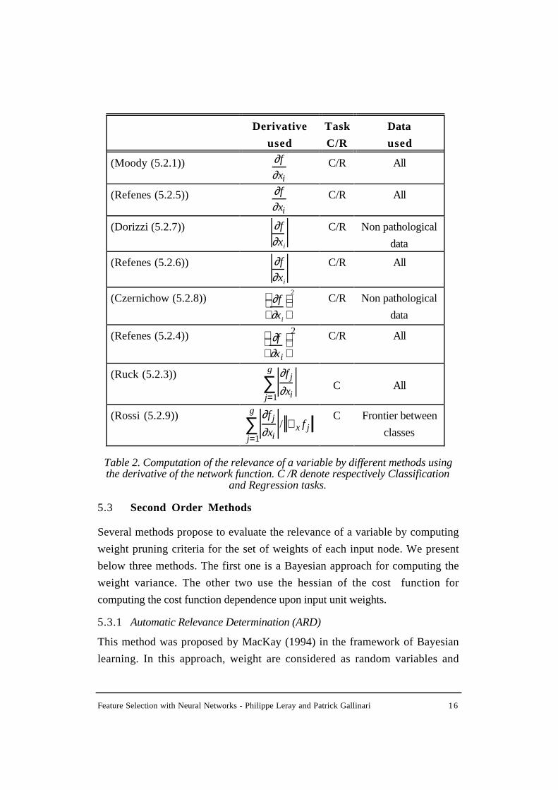
Feature Selection with Neural Networks - Philippe Leray and Patrick Gallinari 16
Derivative
used
Task
C/R
Data
used
(Moody (5.2.1)) ∂f
∂xi
C/R All
(Refenes (5.2.5)) ∂f
∂xi
C/R All
(Dorizzi (5.2.7)) ∂f
∂xi
C/R Non pathological
data
(Refenes (5.2.6)) ∂f
∂xi
C/R All
(Czernichow (5.2.8)) ∂f
∂xi
2C/R Non pathological
data
(Refenes (5.2.4)) ∂f
∂xi
2 C/R All
(Ruck (5.2.3)) ∂f j
∂xij=1
g
∑ C All
(Rossi (5.2.9)) ∂f j
∂xij=1
g
∑ / ∇x f jC Frontier between
classes
Table 2. Computation of the relevance of a variable by different methods usingthe derivative of the network function. C /R denote respectively Classification
and Regression tasks.
5.3 Second Order Methods
Several methods propose to evaluate the relevance of a variable by computing
weight pruning criteria for the set of weights of each input node. We present
below three methods. The first one is a Bayesian approach for computing the
weight variance. The other two use the hessian of the cost function for
computing the cost function dependence upon input unit weights.
5.3.1 Automatic Relevance Determination (ARD)
This method was proposed by MacKay (1994) in the framework of Bayesian
learning. In this approach, weight are considered as random variables and
Feature Selection with Neural Networks - Philippe Leray and Patrick Gallinari 17
regularization terms taking into account each input are included into the cost
function. Assuming that the prior probability distribution of the group of weights
for the ith input is gaussian, the input posterior variance σi2 is estimated (with
the help of the hessian matrix).
ARD has been successful for time serie prediction, learning with regularization
terms improved the prediction performances. However ARD has not really been
used as a feature selection method since variables were not pruned during
training.
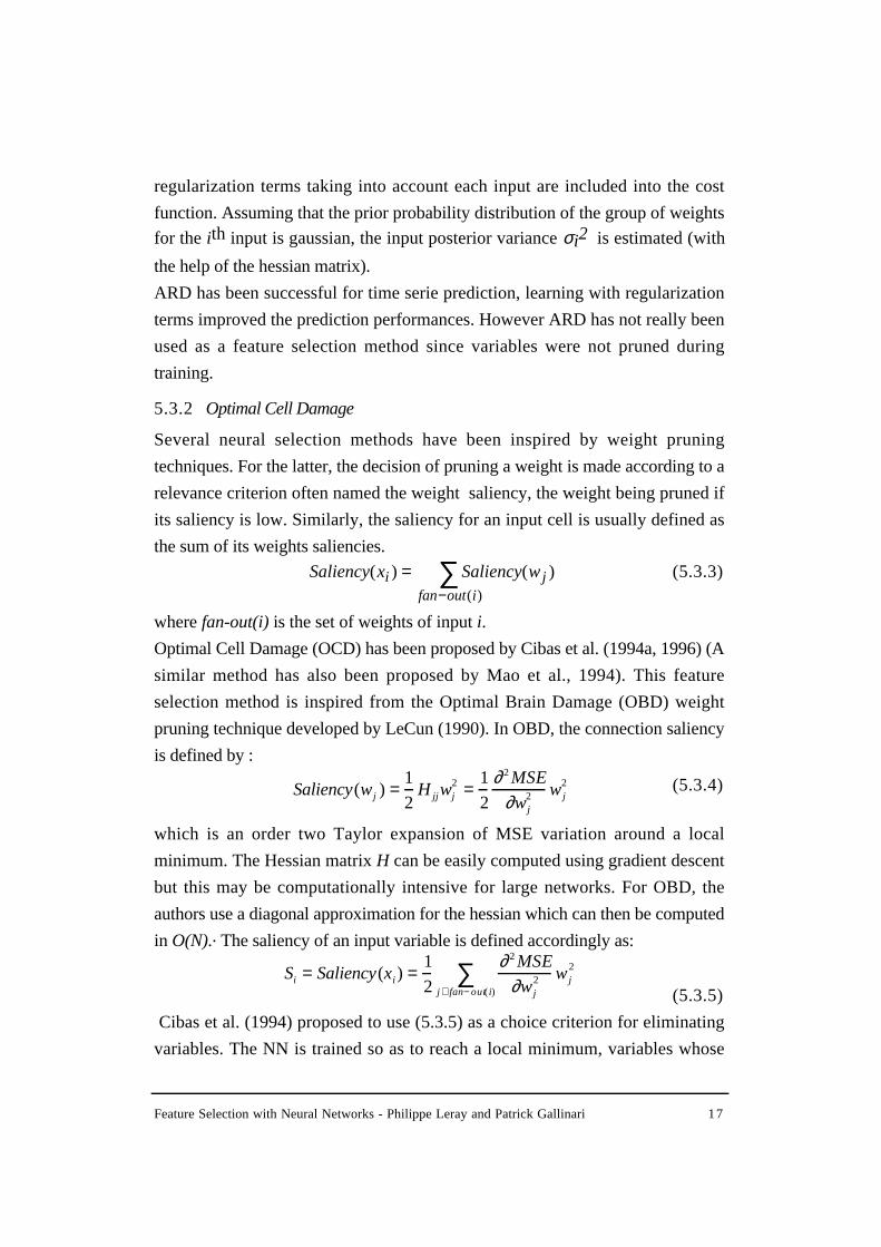
5.3.2 Optimal Cell Damage
Several neural selection methods have been inspired by weight pruning
techniques. For the latter, the decision of pruning a weight is made according to a
relevance criterion often named the weight saliency, the weight being pruned if
its saliency is low. Similarly, the saliency for an input cell is usually defined as
the sum of its weights saliencies.
Saliency(xi ) = Saliency(wj )fan−out(i )
∑ (5.3.3)
where fan-out(i) is the set of weights of input i.
Optimal Cell Damage (OCD) has been proposed by Cibas et al. (1994a, 1996) (A
similar method has also been proposed by Mao et al., 1994). This feature
selection method is inspired from the Optimal Brain Damage (OBD) weight
pruning technique developed by LeCun (1990). In OBD, the connection saliency
is defined by :
Saliency(wj ) =1
2H jj wj
2 =1
2
∂2MSE
∂wj2 wj
2 (5.3.4)
which is an order two Taylor expansion of MSE variation around a local
minimum. The Hessian matrix H can be easily computed using gradient descent
but this may be computationally intensive for large networks. For OBD, the
authors use a diagonal approximation for the hessian which can then be computed
in O(N).. The saliency of an input variable is defined accordingly as:
Si = Saliency(xi ) =1
2
∂2MSE
∂wj2 wj
2
j ∈fan− out( i)∑
(5.3.5)
Cibas et al. (1994) proposed to use (5.3.5) as a choice criterion for eliminating
variables. The NN is trained so as to reach a local minimum, variables whose

Feature Selection with Neural Networks - Philippe Leray and Patrick Gallinari 18
saliency is below a given threshold are eliminated. The threshold value is fixed
by cross validation. This process is then repeated until no variable is found below
the threshold.
This method has been tested on several problems and gave satisfying results.
Once again, the difficulty lies in selecting an adequate threshold. Furthermore,
since several variables can be eliminated simultaneously whereas only individual
variable pertinence measures are used, significant sets of dependent variables
may be eliminated.
For stopping, the generalization performances of the NN sequence are estimated
via a validation set and the variable set corresponding to the NN with the best
performances is chosen.
The hessian diagonal approximation has been questioned by several authors,
Hassibi and Stork (1993), for example, proposed a weight pruning algorithm,
Optimal Brain Surgeon (OBS) which is similar to OBD, but uses the whole
hessian for computing weight saliencies. Stahlberger and Riedmiller (1997)
proposed a feature selection method similar to OCD except that it takes into
account non diagonal terms in the hessian.
For all these methods, saliency is computed using for performance measure the
error variation on the training set. Weight estimation and model selection both use
the same data set, which is not optimal. Pedersen et al. (1996) propose two
weight pruning methods γOBD and γOBS that compute weight saliency
according to an estimate of the generalization error: the Final Prediction Error
(Akaike 1970). Similarly to OBD and OBS, these methods could be also
transformed into feature selection methods.
5.3.3 Early Cell Damage (ECD)
Using a second order Taylor expansion, as in the OBD family of methods, is
justified only when a local minimum is reached and the cost is locally quadratic in
this minimum. Both hypothesis are barely met in practice. Tresp et al. (1997)
propose two weight pruning techniques from the same family, coined EBD
(Early Brain Damage) and EBS (Early Brain Surgeon). They use a heuristic
justification to take into account early stopping by adding a new term in the
saliency computation.

Feature Selection with Neural Networks - Philippe Leray and Patrick Gallinari 19
These methods can be extended for feature ranking, we will call ECD (Early Cell
Damage) the EBD extension. For ECD, the saliency of input i is defined as:
Si =1
2
∂2MSE
∂wj2 wj
2 −j∈ fan−out( i)
∑ ∂MSE
∂wj
wj +1
2
∂MSE
∂wj
2
∂2MSE∂wj
2
(5.3.6)
The algorithm we propose is slightly different from OCD: only one variable is
eliminated at a time, and the NN is retrained after each deletion.
For choosing the "best" set of variables, we have used a variation of the
"selection according to an estimate of the generalization error" method. This
estimate is computed using a validation set. Since the performances may oscillate
and be not significantly different, several subsets may have the same
performances (see e.g. figure 1). Using a Fisher test we compare any model
performances with those of the best model, we then select the set of networks
whose performances are similar to the best ones and choose among these
networks the one with the smallest number of input variables.
6. Experimental comparison
We now present comparative performances of different feature selection
methods. Comparing these methods is a difficult task: there is not a unique
measure which characterizes the importance of each input, the selection accuracy
also depends on the search technique and on the variable subset choice criterion.
In the case of NNs, these different steps rely on heuristics which could be
exchanged from one method to the other. The NNs used are multilayer
perceptrons with one hidden layer of 10 neurons.
The comparison we provide here is not intended for a definite ranking of the
different methods but for illustrating the general behavior of some of the methods
which have been described before. We have used two synthetic classification
problems which illustrate different difficulties of variable selection. In the first
one the frontiers are "nearly" linear and there are dependent variables as well as
pure noise variables. The second problem has non linear frontiers and variables
can be chosen independent or correlated.
Feature Selection with Neural Networks - Philippe Leray and Patrick Gallinari 20
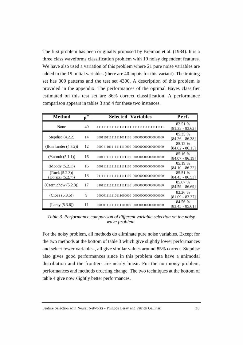
The first problem has been originally proposed by Breiman et al. (1984). It is a
three class waveforms classification problem with 19 noisy dependent features.
We have also used a variation of this problem where 21 pure noise variables are
added to the 19 initial variables (there are 40 inputs for this variant). The training
set has 300 patterns and the test set 4300. A description of this problem is
provided in the appendix. The performances of the optimal Bayes classifier
estimated on this test set are 86% correct classification. A performance
comparison appears in tables 3 and 4 for these two instances.
Method p* Selected Variables Perf.
None 40 111111111111111111111 111111111111111111182.51 %
[81.35 - 83.62]
Stepdisc (4.2.2) 14 000110111111111011100 000000000000000000085.35 %
[84.26 - 86.38]
(Bonnlander (4.3.2)) 12 000011101111111110000 000000000000000000085.12 %
[84.02 - 86.15]
(Yacoub (5.1.1)) 16 000111111111111111100 000000000000000000085.16 %
[84.07 - 86.19]
(Moody (5.2.1)) 16 000111111111111111100 000000000000000000085.19 %
[84.10 - 86.22](Ruck (5.2.3))
(Dorizzi (5.2.7)) 18 011111111111111111100 000000000000000000085.51 %
[84.43 - 86.53]
(Czernichow (5.2.8)) 17 010111111111111111100 000000000000000000085.67 %
[84.59 - 86.69]
(Cibas (5.3.5)) 9 000001111110111000000 000000000000000000082.26 %
[81.09 - 83.37]
(Leray (5.3.6)) 11 000001111111111100000 000000000000000000084.56 %
[83.45 - 85.61]
Table 3. Performance comparison of different variable selection on the noisywave problem.
For the noisy problem, all methods do eliminate pure noise variables. Except for
the two methods at the bottom of table 3 which give slightly lower performances
and select fewer variables , all give similar values around 85% correct. Stepdisc
also gives good performances since in this problem data have a unimodal
distribution and the frontiers are nearly linear. For the non noisy problem,
performances and methods ordering change. The two techniques at the bottom of
table 4 give now slightly better performances.
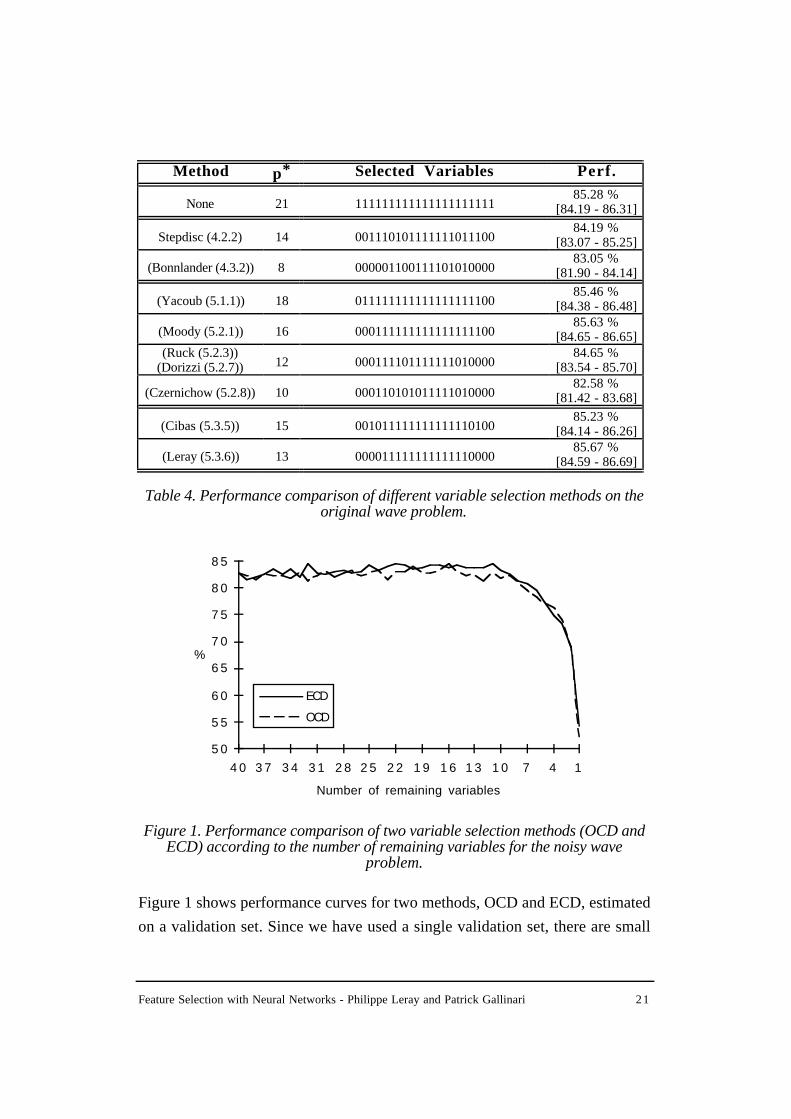
Feature Selection with Neural Networks - Philippe Leray and Patrick Gallinari 21
Method p* Selected Variables Perf.
None 21 11111111111111111111185.28 %
[84.19 - 86.31]
Stepdisc (4.2.2) 14 00111010111111101110084.19 %
[83.07 - 85.25]
(Bonnlander (4.3.2)) 8 00000110011110101000083.05 %
[81.90 - 84.14]
(Yacoub (5.1.1)) 18 01111111111111111110085.46 %
[84.38 - 86.48]
(Moody (5.2.1)) 16 00011111111111111110085.63 %
[84.65 - 86.65](Ruck (5.2.3))
(Dorizzi (5.2.7)) 12 00011110111111101000084.65 %
[83.54 - 85.70]
(Czernichow (5.2.8)) 10 00011010101111101000082.58 %
[81.42 - 83.68]
(Cibas (5.3.5)) 15 00101111111111111010085.23 %
[84.14 - 86.26]
(Leray (5.3.6)) 13 00001111111111111000085.67 %
[84.59 - 86.69]
Table 4. Performance comparison of different variable selection methods on theoriginal wave problem.
Number of remaining variables
%
5 0
5 5
6 0
6 5
7 0
7 5
8 0
8 5
4 0 3 7 3 4 3 1 2 8 2 5 2 2 1 9 1 6 1 3 1 0 7 4 1
ECD
OCD
Figure 1. Performance comparison of two variable selection methods (OCD andECD) according to the number of remaining variables for the noisy wave
problem.
Figure 1 shows performance curves for two methods, OCD and ECD, estimated
on a validation set. Since we have used a single validation set, there are small

Feature Selection with Neural Networks - Philippe Leray and Patrick Gallinari 22
fluctuations in the performances. Some form of cross validation should be used
in order to get better estimates, the test strategy proposed for ECD looks also
attractive in this case. It can be seen that for this problem, performances are more
or less similar during the backward elimination (they slightly rise) until they
quickly drop when relevant variables are removed.
82
84
86
20406080100
None
YacoubMoody
Cibas
Leray
RuckDorizzi
Stepdisc
Bonnlander
Czernichow
%
%
Figure 2. Performance comparison of different variable selection methods vs.percentage of selected variables on the original wave problem. x axis: percentage
of variables selected, y axis: percentage of correct classification.
Figure 2 gives the repartition of different variable selection methods for the
original wave problem according to their performances (y axis) and the
percentage of selected variables (x axis). The best methods are those with the best
performances and the lower number of variables. In this problem, "Leray" is
satisfying (see figure 2). "Yacoub" does not delete enough variables while
"Bonnlander" deletes too much variables.
The second problem is a two class problem in a 20 dimensional space. The
classes are distributed according two gaussians with respectively µ1=(0,...,0),
Σ1=4*I, µ2=(0,1,2,...,19)/α (α is chosen so that ||µ1µ2|| = 2) and Σ2=I . In this
problem, variable relevance is ordered according to their index: x1 is useless,
xi+1 is more relevant than xi.

Feature Selection with Neural Networks - Philippe Leray and Patrick Gallinari 23
Method p* Selected Variables Perf.
None 20 1111111111111111111194.80 %
[94.15 - 94.35]
Stepdisc (4.2.2) 17 1000111111111111111194.88 %
[94.23 - 95.43]
(Bonnlander (4.3.2)) 5 0001000000000001101190.60 %
[89.76 - 91.38]
(Yacoub (5.1.1)) 18 0101111111111111111194.86 %
[94.21 - 95.44]
(Moody (5.2.1)) 9 0100010001100011011192.94 %
[92.20 - 93.62]
(Ruck (5.2.3)) 10 0000000010110111111194.86 %
[94.21 - 95.44]
(Dorizzi (5.2.7)) 11 0000000010111111111194.66 %
[94.00 - 95.25]
(Czernichow (5.2.8)) 9 0000000000110111111194.02 %
[93.33 - 94.02]
(Cibas (5.3.5)) 14 0100111001011111111194.62 %
[93.96 - 95.21]
(Leray (5.3.6)) 15 0101101110111011111194.08 %
[93.39 - 94.70]
Table 5. Performance comparison of different variable selection methods on thetwo gaussian problem with uncorrelated variables.
90
91
92
93
94
95
20406080100
%
%
None
Yacoub Stepdisc
Leray
Cibas DorizziRuck
Czernichow
Moody
Bonnlander
Figure 3. Performance comparison of different variable selection methods vs.percentage of selected variables on the two gaussian problem with uncorrelatedvariables. x axis: percentage of variables selected, y axis: percentage of correct
classification.

Feature Selection with Neural Networks - Philippe Leray and Patrick Gallinari 24
Table 5 shows that Stepdisc is not adapted for this non linear frontier: it is the
only method that selects x1 which is useless for this problem. We can remark on
figure 3 that Bonnlander's method deletes too many variables whereas Yacoub's
stop criterion is too rough and does not delete enough variables.
In an other experiment, we replaced the I matrix in Σ1 and Σ2 by a block
diagonal matrix. Each block is 5x5 so that there are four groups of five
successive correlated variables in the new problem.
Method p* Selected Variables Perf.
None 20 1111111111111111111190.58 %
[89.74 - 91.36]
Stepdisc (4.2.2) 11 0000110101101011011191.96 %
[91.17 - 92.68]
(Bonnlander (4.3.2)) 5 0000100101000010000188.48 %
[85.57 - 89.34]
(Ruck (5.2.3)) 10 0001100101111010001191.06 %
[90.24 - 91.82]
(Leray (5.3.6)) 7 0000001010101010001190.72 %
[89.88 - 91.49]
Table 6. Performance comparison of different variable selection methods on thetwo gaussian problem with correlated variables.
Table 6 gives the results of some representative methods for this problem:
• Stepdisc still gives a model with good performances but selects
many correlated variables,
• Bonnlander's method selects only 5 variables and gives
significantly lower results,
• Ruck's method obtains good performances but selects some
correlated variables,
• Leray's method, thanks to the retraining after each variable deletion,
find models with good performances and few variables (7 compared
to 10 and 11 for Ruck and Stepdisc).

Feature Selection with Neural Networks - Philippe Leray and Patrick Gallinari 25
7. Conclusion
We have reviewed variable selection methods developed in the field of Neural
Networks. The main difficulty here is that NNs are non linear systems which do
not make use of explicit parametric hypothesis. As a consequence, selection
methods rely heavily on heuristics for the three steps of variable selection :
relevance criterion, search procedure - NN variable selection use mainly
backward search - and choice of the final model. We first discussed the main
difficulties for developing each of these steps. We then introduced different
families of methods and discussed their strengths and weaknesses. We believe
that a variable selection method must remain computationally feasible for being
useful, and we have not considered techniques which rely on computer intensive
methods like e.g. bootstrap at each step of the selection . Instead, we have
proposed a series of rules which could be used in order to enhance several of the
methods which have been described, at a reasonable extra computational cost,
e.g. retraining each NN in the sequence and computing the relevance for each of
these NN allows to take into account some correlations between variables, simple
estimates of the generalization error may be used for the evaluation of a variable
subset, simple tests on these estimates, allow to choose minimal variable sets
(section 5.3.3). Finally we performed a comparison of representative NN
selection techniques on synthetic problems.
References
Akaike, H. (1970). Statistical Predictor Identification, Ann. Inst. Statist. Math. 22:203-217.Battiti, R. (1994). Using Mutual Information for Selecting Features in Supervised Neural Net
Learning, IEEE Transactions on Neural Networks 5(4):537-550.Baxt, W.G. and White, H. (1995). Bootstrapping confidence intervals for clinical input variable
effects in a network trained to identify the presence of acute myocardial infraction, NeuralComputation 7:624-638.
Bonnlander, B.V. and Weigend, A.S. (1994). Selecting Input Variables Using MutualInformation and Nonparametric Density Evaluation, in Proceedings of ISANN'94. 42-50.
Breiman, L., Friedman, J., Olshen R., and Stone, C. (1984). Classification and RegressionTrees. Wadsworth International Group.
Cibas, T. Fogelman Soulié, F. Gallinari, P. and Raudys, S. (1994a). Variable Selection withOptimal Cell Damage. In Proceedings of ICANN'94.
Cibas, T. Fogelman Soulié, F. Gallinari, P. and Raudys, S. (1996). Variable Selection withNeural Networks. Neurocomputing 12:223-248.
Czernichow, T. (1996). Architecture Selection through Statistical Sensitivity Analysis. InProceedings of ICANN'96, Bochum, Germany.
Feature Selection with Neural Networks - Philippe Leray and Patrick Gallinari 26
Dorizzi, B. Pellieux, G. Jacquet, F Czernichow, T. and Munoz, A. (1996). Variable SelectionUsing Generalized RBF Networks : Application to the Forecast of the French T-Bonds. InProceedings of IEEE-IMACS'96, Lille, France.
Fraser, A.M. and Swinney, H.L. (1986). Independent Coordinates for Strange Attractors fromMutual Information, Physical Review A:33(2):1134-1140.
Goutte, C. (1997). Extracting the Relevant Decays in Time Series Modelling, Neural Networksfor Signal Processing VII, Proceedings of the IEEE Workshop, Neural Networks for SignalProcessing VII, Proceedings of the IEEE Workshop.
Gustafson and Hajlmarsson (1995). 21 maximum likelihood estimators for model selection.Automatica.
Habbema, J.D.F and Hermans, J. (1977). Selection of Variables in Discriminant Analysis byF-statistic and Error Rate, Technometrics, 19(4):487-493.
Härdle, W. (1990). Applied Nonparametric Regression. Cambridge University Press.Econometric Society Monograph n.19.
Hashem, S. (1992). Sensitivity Analysis for Feedforward Artificial Neural Networks withDifferentiable Activation Functions. In Proceedings of 1992 International Joint Conferenceon Neural Networks IJCNN92 I:419-424.
Hassibi, B. and Stork, D.G. (1993). Second Order Derivatives for Network Pruning : OptimalBrain Surgeon. Neural Information Processing Systems 5:164-171.
Kittler, J. (1986). Feature Selection and Extraction, Chapter 3 in Handbook of PatternRecognition and Image Processing, Eds. Tzay Y. Young, King-Sun Fu, Academic Press.59-83.
Larsen, J. and Hansen, L.K. (1994). Generalized performances of regularized neural networksmodels. Proceedings of the 1994 IEEE Workshop on Neural Networks for SignalProcessing. 42-51.
LeCun, Y. Denker, J.S. and Solla, S.A. (1990). Optimal Brain Damage. Neural InformationProcessing Systems 2:598-605.
MacKay, D.J.C. (1994). Bayesian Non-linear Modelling for the Energy PredictionCompetition. In ASHRAE Transactions. 1053-1062.
Mao, J. Mohiuddin, K. and Jain, A.K. (1994). Parsimonious Network Design and FeatureSelection Through Node Pruning. In Proceedings of the 12th International Conference onPattern Recognition. 622-624.
McLachlan, G.J. (1992). Discriminant Analysis and Statistical Pattern Recognition, Wiley-Interscience publication.
Moody, J. (1991). Note on generlization, regularization and architecture selection in non linearlearning systems. Proceedings of the first IEEE Workshop on Neural Networks for SignalProcessing. 1-10.
Moody, J. and Utans, J. (1992). Principled Architecture Selection for Neural Networks:Application to Corporate Bond Rating Prediction. Neural Information Processing Systems4.
Moody, J. (1994). Prediction Risk and Architecture Selection for Neural Networks in FromStatistics to Neural Networks - Theory and Pattern Recognition Applications, Eds V.Cherkassky, J.H. Friedman, H. Wechsler, Springer-Verlag.
Narendra, P.M. and Fukunaga, K. (1977). A Branch and Bound Algorithm for Feature SubsetSelection. IEEE Transactions on Computers 26(9):917-922.
Pedersen, M.W. Hansen, L.K. and Larsen, J. (1996). Pruning with generalisation based weightsaliencies: γOBD, γOBS. Neural Information Processing Systems 8.
Priddy, K.L. Rogers, S.K. Ruck, D.W. Tarr, G.L. and Kabrisky, M. (1993). BayesianSelection of Important Features for Feedforward Neural Networks. Neurocomputing 5:91-103. Elsevier ed.
Pudil, P., Novovicova, J. and Kittler, J. (1994). Floating search methods in feature selection.Pattern Recognition Letters 15:1119-1125.

Feature Selection with Neural Networks - Philippe Leray and Patrick Gallinari 27
Refenes, A.N. Zapranis, A. and Utans J. (1996). Neural Model Identification, VariableSelection and Model Adequacy. In Neural Networks in Financial Engineering, Proceedingsof NnCM-96.
Rossi, F. (1996). Attribute Suppression with Multi-Layer Perceptron. In Proceedings of IEEE-IMACS'96, Lille, France.
Ruck, D.W. Rogers, S.K. and Kabrisky, M. (1990). Feature Selection Using a MultiLayerPerceptron. In J. Neural Network Comput. 2 (2):40-48.
Stahlberger, A. and Riedmiller, M. (1997). Fast Network Pruning and Feature Extraction Usingthe Unit-OBS Algorithm. Neural Information Processing Systems 9:655-661.
Thompson M.L. (1978). Selection of Variables in Multiple Regression. Part I: A Review andEvaluation, International Statistical Review, 46:1-19, Selection of Variables in MultipleRegression. Part II: Chosen Procedures, Computations and Examples, in InternationalStatistical Review, 46:129-146.
Tresp, V. Neuneier, R. and Zimmermann, G. (1997). Early Brain Damage. Neural InformationProcessing Systems 9:669-675.
Van de Laar, P. Gielen, S. and Heskes, T. (1997). Input Selection with Partial Retraining. InProceedings of ICANN'97.
White, H. (1989). Learning in Artificial Neural Networks : A Statistical Perspective. NeuralComputation 1:425-464.
Wilks, S.S. (1963). Mathematical Statistics, Wiley, New York.Yacoub, M. and Bennani, Y. (1997). HVS: A Heuristic for Variable Selection in Multilayer
Artificial Neural Network Classifier. in Proceedings of ANNIE'97. 527-532.
Appendix : waveforms problem
This problem has been proposed by Breiman et al. (1984). 3 vectors or
waveforms in 21 dimensions, Hi, i = 1, …, 3, are given. Patterns in each class
are defined in ℜ21 as random convex combinations of 2 of these vectors (waves
(1,2), (1,3), (2,3) respectively for class 1, 2 and 3).
The problem is then to classify these patterns into one of the 3 classes. More
precisely, patterns are generated according to:
xi = uHim + (1− u)Hi
n
5+ εi
0 ≤ i ≤ 20
where xi denotes the ith component of a pattern x, u is a uniform random variable
in [0,1], εi is generated according to a normal distribution N(0,1), m and n
identify the two waves used in this combination, i.e. the class of pattern x.
For the noisy problem, 19 additional components are added to the 21 components
of the above vectors:xi = εi 21 ≤ i ≤ 40
The training, validation and test sets have respectively 300, 1000, 4300 elements.


