10.1.1.12.510

8/7/2019 10.1.1.12.510

http://slidepdf.com/reader/full/101112510 1/10

Header for SPIE use

Segmentation of medical images using adaptive region growingRegina Pohle*, Klaus D. Toennies

Otto-von-Guericke University Magdeburg, Department of Simulation and Graphics

ABSTRACTInteraction increases flexibility of segmentation but it leads to undesirable behavior of an algorithm if knowledge being

requested is inappropriate. In region growing, this is the case for defining the homogeneity criterion, as its specification

depends also on image formation properties that are not known to the user. We developed a region growing algorithm that

learns its homogeneity criterion automatically from characteristics of the region to be segmented. The method is based on a

model that describes homogeneity and simple shape properties of the region. Parameters of the homogeneity criterion are

estimated from sample locations in the region. These locations are selected sequentially in a random walk starting at the

seed point, and the homogeneity criterion is updated continuously. This approach was extended to a fully automatic and

complete segmentation method by using the pixels with the smallest gradient length in the not yet segmented image region

as a seed point. The methods were tested for segmentation on test images and of structures in CT and MR images. We found

the methods to work reliable if the model assumption on homogeneity and region characteristics are true. Furthermore, the

model is simple but robust, thus allowing for a certain degree of deviation from model constraints and still delivering the

expected segmentation result.

Keywords: segmentation, region growing, adaptive methods

1. INTRODUCTION

Often the analysis of medical images for the purpose of computer-aided diagnosis and therapy planning contains a

segmentation as a preliminary stage for the visualization or quantification. For medical CT and MR images, many methods

were recently employed for segmentation, for instance interactive thresholding aided by morphological information [1],

region growing and region splitting and merging [2,3], active contours [4,5,6,7], the use of cluster analysis methods

[8,9,10], or watershed transformation [11,12,13]. In the individual segmentation methods different complex models of the a-

priori information about the expected contents of the image are used. The applied a-priori knowledge consists of a

combination of anatomical/physiological information and of information about the image formation process. The more the

contributed model information is verifiable, the more likely is the possibility of automation of the segmentation process.

Also, the result of the algorithm can be predicted easier. Especially in medical segmentation tasks the model information isoften too complex or not exact to specify so that a completely automatic extraction is not possible. The aim of the

development of a segmentation method should be to minimize the part of the interactively introduced model information

and to maximize the part of the automatically analyzed model information. Model information should be supplied

interactively only in those cases where it represents knowledge that is readily available to the user and where it can be

entered in a robust fashion. Contravening this rule may cause reactions of the process to user interaction which are

perceived as being inconsistent with the user’s expectations.

As an example for such contravention, we consider the simple region growing. A successful specification of a structure in a

medical image requires information on a seed location and specification of region homogeneity characteristics. The former

presents no problems to the user. Because of his anatomical knowledge the user can easily pinpoint the seed location to

segment a certain structure in the image. The input of the region homogeneity characteristics is more difficult because the

homogeneity criterion may not be immediately perceivable to the user. He has often a vague and fuzzy concept of

homogeneity and this concept is not translated easily into a computable criterion. Consequently, so far defininghomogeneity is a tedious trial-and-error process. The simple region growing method is also an example for a contravention

of the rule of the robust interactive input of model information. For the improvement of the region growing segmentation

process various simplifications were developed for selecting the homogeneity criterion automatically from the image. Law

and Heng [14] developed a method of iteratively incrementing the deviation. As optimal threshold the value is selected after

that the number of member pixels of the region suddenly increased. This approach requires long computation times if the

objects to be segmented are large and if the start value of the homogeneity criterion is far from the real value. Another

possible error is the overestimation of the region size in case that the region is beginning to leak out only at some points. In

[15], upper and lower boundaries for the deviation are extracted from histograms of a set of slices. The method can applied

only if few objects with similar or overlapping gray value ranges are present in the image. The main problem of such

measures is the use of an insufficient model for homogeneity. Therefore, the predictions of the system’s behavior based on

8/7/2019 10.1.1.12.510


region characteristics is difficult. Knowing about this fact, we developed a new adaptive region growing method. Our method learns its homogeneity criterion on a model of regions and their homogeneity while searching for the region. As

criterion for the homogeneity we use the gray value of the region and standard deviation, similar to [16,17], assuming that

the variation of the gray values within regions is smaller than that between regions. We think that the model is robust

because the homogeneity criterion contains only information about the region itself.

2. DERIVATION OF THE HOMOGENEITY MODEL FROM MEDICAL IMAGESThe objective of our work is the development of a simple and robust possibility to describe the homogeneity criterion in a

simple form. This description method is to be used for segmentation of 2D and 3D structures in CT and MR data. Our

knowledge of the homogeneity model is based on knowledge about the image formation process. In CT images values of the

image represent average x-ray absorption distorted by noise and artifacts. The absorption itself is assumed to be constant for

a given anatomical structure. The noise is assumed to be zero mean gaussian noise with an unknown standard deviation. For

CT images, the main artifact is assumed to be the partial volume effect (PVE). In contrast to the CT images, signalintensities in MR images are influenced by several overlapping relaxation processes. Beside noise artifacts and partial

volume effect, other problems like shading effects complicated segmentation.

Homogeneity without visible shading may be defined as likelihood of belonging to a gaussian distribution of gray values

with a given mean and standard deviation. The mean is the absorption value of the tissue in CT images and the

magnetization in MR images. The standard deviation accounts for variations due to noise (this criterion was used as

homogeneity measure by other authors, e.g., [16, 17]). The effects of the PVE can be captured in an approximative fashionby assuming different “standard deviations” for gray values that are higher or lower than the mean.

The appropriateness of this model was tested by investigating grey level distributions of CTs and MRs of the abdomen

along a manually marked line (see Figure 1). The asymmetry of the distribution due to the PVE can be seen clearly in the

gray level histogram of the manually segmented regions in both images. Its degree depends on the gray values of the

surrounding tissue of a region. If the average of gray levels of the surrounding tissues is equal to the mean gray value of the

region, then the distribution should be approximately gaussian and symmetric. If the surrounding tissue is on average darker

or lighter than the mean of the region then asymmetry develops as it can be seen in Figure 1.

Fig. 1: Top: CT image of the abdomen (left), gray levels along line A-B (center) and gray level histograms of the liver

region (right); Bottom: MR image of the abdomen (left), gray levels along line A-B (center), and gray level histograms of

the left kidney region (right).

8/7/2019 10.1.1.12.510


3. THE ADAPTIVE REGION GROWING ALGORITHM FOR SEMI-AUTOMATIC

SEGMENTATION

A connected region is found by region growing on condition that the seed point (the first pixel) is set into the region, on

condition that each neighbor of every active pixel is investigated for region membership and on condition that the

homogeneity criterion remains unchanged throughout the region growing process. In order to reduce necessary interaction,

we want to apply region growing also as a learning process for finding the homogeneity parameters. As these parameters

change during learning, the adaptive process requires two runs of region growing. In the first run, homogeneity parametersare estimated, and they are applied, using the same seed point, in a second run for extracting the region.

Learning the homogeneity criterion defined previously requires to estimate mean and two different standard deviations for

gray values of a number of pixels of the region. Since the combination of two halves of two different gaussian functions is

not a gaussian, the mean needs to be estimated from the median instead of the average of the pixel values. The two standard

deviations are then estimated by separately evaluating gray values of the sample pixels that are greater or lower than the

mean.

During early stages of the learning process, the current estimate for homogeneity should be weakly applied for deciding on

region membership in order to avoid premature termination of the process because the standard deviation is underestimated.

Given the deviations ld and ud that were computed at a previous step of the region growing procedure, lower and upper

thresholds are computed for determining region membership:

( ) ( ) ( )[ ] ( ) ( ) ( )[ ]ncwnld nmgvT and ncwnud nmgvT lower upper +⋅−=+⋅+= (1)

The value n stands for the number of pixels that were used to compute the estimate. The weight w was set to 1.5 to include

approximately 86% of all region members if the distribution was truly gaussian. The weight was set this low in order to

avoid leaking out of the region and thus delivering the wrong estimate. The unreliability of the estimates of mgv, ud and ld at early stages of the learning process was compensated for by a function c(n) that decreases with increasing n. It was

chosen as ( )n

nc 20= , which rapidly decreases with increasing n. Initial values for mgv, ud and ld are estimated from a 3x3

neighborhood around the seed point.

Estimating region characteristics of a yet undetermined region will succeed only if a reliable estimate of the homogeneity

parameters can be given before the first non-region pixel is considered. Fortunately, the number of pixels for achieving

reliability needs not be large because only three parameters have to be estimated. Three assumptions were made for creatinga search process that avoids premature encountering of the region boundary:

1. The user sets the seed point not close to the region boundary.

2. The region consists of pixels, sufficient in number for a reliable estimate of homogeneity.

3. The region is compact, i.e., circle-shaped rather than elongated.

On these assumptions the standard region growing technique is inappropriate for the first run as it follows the region in one

direction until the region boundary is found, and then chooses a new direction. Instead, we chose the order of visiting

neighbors at random each time. It produces a search order which closely resembles a random walk starting at the seed point

(Figure 2).

Fig. 2: Randomized region growing after seed point setting and visiting 9, 40, 100, 150, 200, 300, 400 and 475 pixels.

Parameters of the homogeneity are re-computed each time the number of pixels in the training region has doubled. After

termination, the two deviations ld and ud have to be adjusted in order to account for the constant underestimation of the

standard deviation by using only pixels in the training region that deviate by less than 1.5·w from the current mean. The

extent of this underestimation can be computed from tabulated integrals of the gaussian curve. The resulting correction

factors are listed in Table 1.

8/7/2019 10.1.1.12.510


For the second run, the region growing process is repeated using the same seed point, the estimated mean and the correctedstandard deviations. The weight w was set to w=2.58 in order to include 99% of the pixels of the region if the variation due

to noise was truly gaussian.

Number of updates of the estimated

standard deviation

1 2 3 4 5 6 7 8

Correction factor for std dev 1.0 1.14 1.29 1.43 1.58 1.72 1.90 2.05

Table 1: The standard deviation is updated each time the region size has doubled. As new pixels are included only if they

deviate by less than 1.5 times the standard deviation, the true standard deviation is more and more underestimated. The

correction factor takes this into account.

4. EXTENSION OF THE ALGORITHM FOR THE AUTOMATIC SEGMENTATION

The approach of the adaptive region growing can be extended to a fully automatic and complete segmentation method of

medical images. In this case, pixels are selected as seed points that have the smallest gradient length and that are not yet part

of a segmented image region. Using the smallest gradient value as actual seed point, we can be sure that the seed point is

always located within a region because the variation of the gray values within regions is assumed to be smaller than the

variation between regions. Overlapping regions are not allowed during the region growing process. In contrast to the semi-automatic segmentation in the second run, the region growing process was repeated with weight of w=2.0 (instead of

w=2.58) in order to include only 95% of the pixels of the region for a strict avoidance of leakage of the regions. The

segmentation process stops if each pixel belongs to a region. Because of the partial volume effect in most images, the

homogeneity criterion is not met in the boundary areas between different regions. In these areas new separate regions are

developed as can be seen in Figure 3. Result of this process is a over-segmentation of the image. Therefore, over-segmented

regions must be removed in the next step. The probability of a segment being an anatomically meaningful region increases

with its homogeneity, compactness and size. Thus, we defined that the region probability is dependent on a size and shape-

dependent probability PS and a homogeneity-dependent probability PH.

H S RegionP P P ⋅= (2)

The region only continues to exist if both probabilities are high because we multiply this values.

4.1 DETERMINATION OF THE REGION PROBABILITYThe region size and shape is assessed using a morphologic opening operation. To begin, the region size S1 is determined

after the segmentation process. Then an erosion and dilatation operation starts. The resulting region size S2 after opening is

calculated. The region probability is computed from S1 and S2 as follows:

ïî

ïíì

≤=

otherwise

S S

if S

S P S

,1

1,1

2

1

2 (3)

Fig. 3: Result of the first step of automatic

segmentation for marked region in a CT image of

the abdomen. Many over-segmented regions can

be seen in the boundary area of the kidney.

8/7/2019 10.1.1.12.510


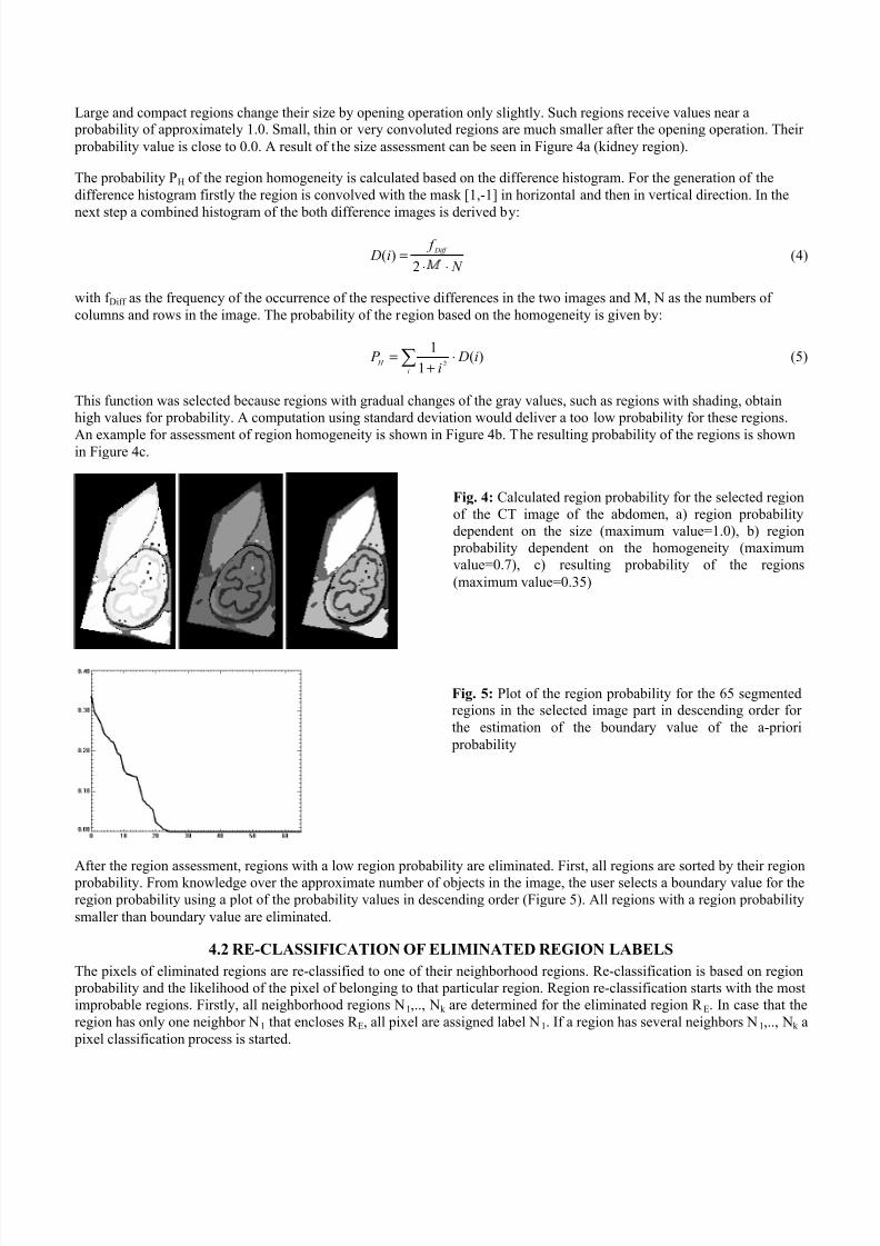
Large and compact regions change their size by opening operation only slightly. Such regions receive values near aprobability of approximately 1.0. Small, thin or very convoluted regions are much smaller after the opening operation. Their

probability value is close to 0.0. A result of the size assessment can be seen in Figure 4a (kidney region).

The probability PH of the region homogeneity is calculated based on the difference histogram. For the generation of the

difference histogram firstly the region is convolved with the mask [1,-1] in horizontal and then in vertical direction. In the

next step a combined histogram of the both difference images is derived by:

N

f iD

Diff

⋅⋅=

2)( (4)

with f Diff as the frequency of the occurrence of the respective differences in the two images and M, N as the numbers of

columns and rows in the image. The probability of the region based on the homogeneity is given by:

å ⋅+

=

i

H iD

iP )(

1

12

(5)

This function was selected because regions with gradual changes of the gray values, such as regions with shading, obtain

high values for probability. A computation using standard deviation would deliver a too low probability for these regions.

An example for assessment of region homogeneity is shown in Figure 4b. The resulting probability of the regions is shownin Figure 4c.

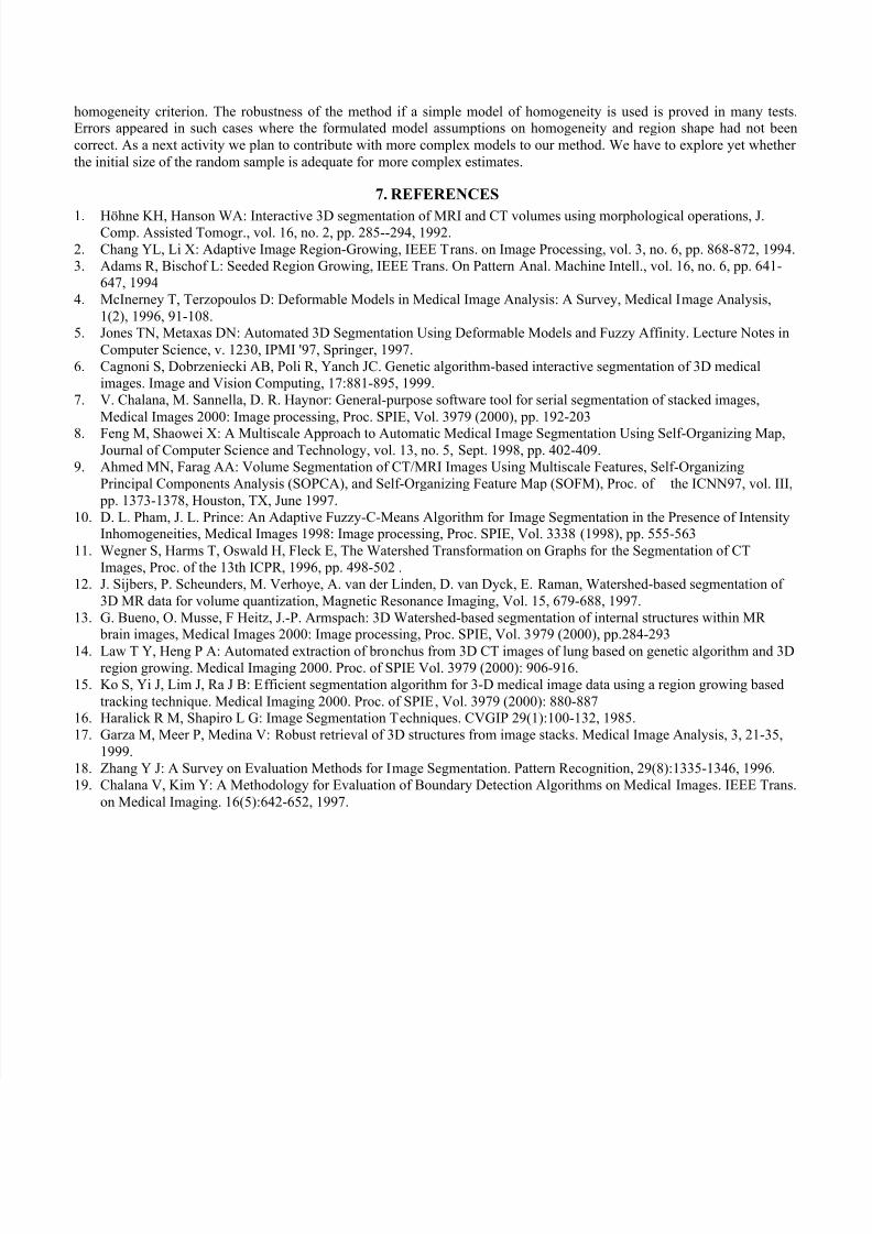
After the region assessment, regions with a low region probability are eliminated. First, all regions are sorted by their regionprobability. From knowledge over the approximate number of objects in the image, the user selects a boundary value for the

region probability using a plot of the probability values in descending order (Figure 5). All regions with a region probability

smaller than boundary value are eliminated.

4.2 RE-CLASSIFICATION OF ELIMINATED REGION LABELS

The pixels of eliminated regions are re-classified to one of their neighborhood regions. Re-classification is based on region

probability and the likelihood of the pixel of belonging to that particular region. Region re-classification starts with the most

improbable regions. Firstly, all neighborhood regions N1,.., Nk are determined for the eliminated region R E. In case that the

region has only one neighbor N1 that encloses R E, all pixel are assigned label N1. If a region has several neighbors N1,.., Nk a

pixel classification process is started.

Fig. 4: Calculated region probability for the selected region

of the CT image of the abdomen, a) region probability

dependent on the size (maximum value=1.0), b) region

probability dependent on the homogeneity (maximum

value=0.7), c) resulting probability of the regions

(maximum value=0.35)

Fig. 5: Plot of the region probability for the 65 segmentedregions in the selected image part in descending order for

the estimation of the boundary value of the a-priori

probability

8/7/2019 10.1.1.12.510


For every neighborhood region Ni, the probability distribution PNi of the gray values is generated from the median value and

from the lower and upper standard deviation. Then, for every pixel of the eliminated region a membership probability P g∈N

is determined depending on the gray value of the pixel. This procedure is shown for the example region R E in Figure 6. Theregion probability was 0.278 for neighbor N0, 0.094 for neighbor N1 and 0.005 for neighbor N2. In Figure 7 the distribution

function of all neighborhood regions and the derived probabilities Pg∈N0, Pg∈N1 and Pg∈N2 are shown.

Fig. 7: Distribution functions for the three neighborhood regions and derived probabilities for the considered pixel in Fig. 6

with a gray value of 1216.

The re-classification of the pixels to a region Ni depends on a contribution on the overall probability PRegion of Ni, according

to Equation 2, and on the probability Pg(p)∈N of the pixel p with a gray value g(p) of belonging to that distribution:

( )ig Region P P N ∈⋅= max , with i= N1,.., Nk (6)

The considered pixel in Figure 6 was classified as class N 2. After the classification process we must determine whether all

regions are connected. If pixels of the region are classified so that no connection to the neighborhood region exists, a new

assignment to a less probable neighborhood region will be tried until a connection was secured. This process is illustrated in

Figure 8.

Fig. 8: a) Demonstration of the connection test for the white labeled region, b) enlarged image of the marked region, c)

region after re-classification, d) region after connection test

N0N1

R E

N2

Fig. 6: Part of the CT image of the abdomen (left)and produced segmentation result (right), region R Eshould be eliminated and pixels should be re-

classified to one of the neighborhood regions N0,..,

N2.

Pg∈∈∈∈N0=0.0 Pg∈∈∈∈N1=0.04 Pg∈∈∈∈N2=0.37

a)

b) c) d)

8/7/2019 10.1.1.12.510


5. RESULTS

The performance of our new segmentation algorithm was evaluated with empirical discrepancy methods. The quality

measure is determined indirectly based on the results of the algorithm by test images. We have selected discrepancy

methods because an objective and quantitative assessment of the segmentation algorithm is possible with a close

relationship to a concrete application. As error metrics we have used the average deviation between the contour pixels andthe contour in the gold standard, Hausdorff distance, number of over-segmented and under-segmented pixels in relation to

the region size [18,19].

In a first test we investigated what degree of deviation from our homogeneity model the semi-automatic algorithm would

tolerate. For this purpose we created artificial test images which contained, in gradations, the influences to be examined. In

medical images segmentation is influenced through variation of the signal-to-noise relation (SNR), variation of the object

shape, modification of the edge gradient as simulation of the partial volume effect, and modification of the shading. The

first three criteria are part of our homogeneity model. The last criterion is not part of the model but may well occur inreality. An example for the used test images can be seen in Figure 9. For a better simulation of the real conditions, we have

extracted noise from the homogenous areas in CT images, instead of using artificial noise. This noise was overlaid test

images with different other conditions, like contrast, edge gradient, or shading.

Figure 10: Results of the discrepancy measurement of the average error, average of each time six runs per measuring point.

Top left: for the segmentation of test images with variation of the SNR, top right: for the segmentation of test images with

variation of the object shape (length-width-ratio), bottom left: for the segmentation of test images with variation of the edge

gradient, bottom right: for the segmentation of test images with variation of the shading.

Fig. 9: Starting image (object diameter: 60 pixels),

image with the extracted noise signal, test image for a

SNR of 1.5:1, result of the first run, end result.

8/7/2019 10.1.1.12.510


In all tests we have ascertained that all error metrics had similar trends. For the investigation of the influence of the signal-to-noise relation the results for a SNR higher than 1.5:1 show that the average deviation between contour pixels was below

0.5 pixel and the maximum deviation was three pixels on average. For the investigation of the influence of the shape, edge

gradient and shading results show that at very narrow objects, with increased edge smoothing and increased shading, the

error increased significantly. As an example for results of discrepancy measurement you can see the results for average error

in Figure 10.

Then, we investigated whether the outcome on test images helped predicting the performance on real medical images if

compared to manual segmentation. We have segmented two structures in CT images with five different seed point locations,

liver with a SNR of 1.5:1 and passable lumen of the aortic aneurysm with a SNR of 5:1. For assessing the quality of theresults, we compared them with a manual segmentation that was carried out by a practicing surgeon. Results of

segmentation are shown in Figure 11 and Table 2. As an example for segmentation in MR images you can see a segmented

kidney region in Figure 12.

metrics for error evaluation liver passable lumen

average error 1.09 ± 0.06 1.45 ± 0.17

Hausdorff distance 3.62 ± 0.34 4.63 ± 0.62

oversegmented pixels in % 1.46 ± 0.30 0.08 ± 0.00

not segmented pixels in % 5.66 ± 0.71 10.28 ± 1.27

In a next step we have tested automatic region growing algorithm by applying it to CT images of the abdomen and to

magnetic resonance brain images. In both cases the segmentation process led to good results by visual assessment. The

result for a brain image is shown in Figure 13, and the result for the CT region in Figure 14. In the first step of the automatic

region growing, the brain image is split into 557 regions. After the elimination of the regions with a low region probability,

121 regions are in this image. In the considered area of the CT image 67 regions after the first step are reduced to 14 result

regions.

Fig. 11: Segmentation results of the semi-automatic adaptive region

growing method for the liver and passable lumen of the aortic

aneurysm. Segmented regions are labeled black.

Table 2: Measured values for a

comparison of the segmentation results

with the regions manually segmented.

Fig. 12: Segmentation results of the semi-automatic adaptive region

growing method for the left kidney in MR images of the abdomen.

Segmented regions are labeled white in the slice.

8/7/2019 10.1.1.12.510


Fig. 13: Segmentation result for automatic algorithm for a brain MR image: a) original MR image, b) result after automatic

segmentation, c) labeling result after re-classification, d) regions are coded with their average gray value

6. CONCLUSION

In this paper, we presented a new self-learning, fully automatic approach for a region-oriented segmentation of medical

images. In contrast to other complete segmentation methods, like the watershed transformation and split-and-merge

algorithm, the connectivity of regions is better preserved. Moreover, our method allows a region-specific variation of the

Fig. 14: Segmentation result for automatic segmentation for region in

CT image of the abdomen; left:

original image, center: regions are

coded with labels, right: regions arecoded with their average gray value.

8/7/2019 10.1.1.12.510


homogeneity criterion. The robustness of the method if a simple model of homogeneity is used is proved in many tests.Errors appeared in such cases where the formulated model assumptions on homogeneity and region shape had not been

correct. As a next activity we plan to contribute with more complex models to our method. We have to explore yet whether

the initial size of the random sample is adequate for more complex estimates.

7. REFERENCES

1. Höhne KH, Hanson WA: Interactive 3D segmentation of MRI and CT volumes using morphological operations, J.Comp. Assisted Tomogr., vol. 16, no. 2, pp. 285--294, 1992.

2. Chang YL, Li X: Adaptive Image Region-Growing, IEEE Trans. on Image Processing, vol. 3, no. 6, pp. 868-872, 1994.

3. Adams R, Bischof L: Seeded Region Growing, IEEE Trans. On Pattern Anal. Machine Intell., vol. 16, no. 6, pp. 641-

647, 1994

4. McInerney T, Terzopoulos D: Deformable Models in Medical Image Analysis: A Survey, Medical Image Analysis,

1(2), 1996, 91-108.5. Jones TN, Metaxas DN: Automated 3D Segmentation Using Deformable Models and Fuzzy Affinity. Lecture Notes in

Computer Science, v. 1230, IPMI '97, Springer, 1997.

6. Cagnoni S, Dobrzeniecki AB, Poli R, Yanch JC. Genetic algorithm-based interactive segmentation of 3D medical

images. Image and Vision Computing, 17:881-895, 1999.

7. V. Chalana, M. Sannella, D. R. Haynor: General-purpose software tool for serial segmentation of stacked images,

Medical Images 2000: Image processing, Proc. SPIE, Vol. 3979 (2000), pp. 192-203

8. Feng M, Shaowei X: A Multiscale Approach to Automatic Medical Image Segmentation Using Self-Organizing Map,Journal of Computer Science and Technology, vol. 13, no. 5, Sept. 1998, pp. 402-409.

9. Ahmed MN, Farag AA: Volume Segmentation of CT/MRI Images Using Multiscale Features, Self-Organizing

Principal Components Analysis (SOPCA), and Self-Organizing Feature Map (SOFM), Proc. of the ICNN97, vol. III,

pp. 1373-1378, Houston, TX, June 1997.

10. D. L. Pham, J. L. Prince: An Adaptive Fuzzy-C-Means Algorithm for Image Segmentation in the Presence of IntensityInhomogeneities, Medical Images 1998: Image processing, Proc. SPIE, Vol. 3338 (1998), pp. 555-563

11. Wegner S, Harms T, Oswald H, Fleck E, The Watershed Transformation on Graphs for the Segmentation of CT

Images, Proc. of the 13th ICPR, 1996, pp. 498-502 .

12. J. Sijbers, P. Scheunders, M. Verhoye, A. van der Linden, D. van Dyck, E. Raman, Watershed-based segmentation of

3D MR data for volume quantization, Magnetic Resonance Imaging, Vol. 15, 679-688, 1997.

13. G. Bueno, O. Musse, F Heitz, J.-P. Armspach: 3D Watershed-based segmentation of internal structures within MR brain images, Medical Images 2000: Image processing, Proc. SPIE, Vol. 3979 (2000), pp.284-293

14. Law T Y, Heng P A: Automated extraction of bronchus from 3D CT images of lung based on genetic algorithm and 3Dregion growing. Medical Imaging 2000. Proc. of SPIE Vol. 3979 (2000): 906-916.

15. Ko S, Yi J, Lim J, Ra J B: Efficient segmentation algorithm for 3-D medical image data using a region growing based

tracking technique. Medical Imaging 2000. Proc. of SPIE, Vol. 3979 (2000): 880-88716. Haralick R M, Shapiro L G: Image Segmentation Techniques. CVGIP 29(1):100-132, 1985.

17. Garza M, Meer P, Medina V: Robust retrieval of 3D structures from image stacks. Medical Image Analysis, 3, 21-35,

1999.

18. Zhang Y J: A Survey on Evaluation Methods for Image Segmentation. Pattern Recognition, 29(8):1335-1346, 1996.

19. Chalana V, Kim Y: A Methodology for Evaluation of Boundary Detection Algorithms on Medical Images. IEEE Trans.

on Medical Imaging. 16(5):642-652, 1997.

10.1.1.12.510

Documents

Transcript of 10.1.1.12.510