10. Numerical Integration - Galileogalileo.phys.virginia.edu/compfac/courses/practical-c/10.pdf ·...

10. Numerical Integration

10.1. IntroductionSometimes a problem in Science or Engineering allows us to find an

elegant solution that represents a simple, exact answer. Mathematics

tells us that the area of a circle is exactly πr2. We know that the distance

travelled by an uniformly accelerating body is v0t + 12 at2.

Figure 10.1: Isaac Newton in 1689.Source: Wikimedia Commons

Calculus (first called the “calculus ofinfinitesimals”) was co-invented inthe 17th Century by Gottfried Wilhelmvon Leibniz in Germany and IsaacNewton in England. The two arguedbitterly over which of them deservedcredit. The Royal Society of Londonformed a committee chaired by Newtonto investigate the dispute, and itsreport (written by Newton) ruled,unsurprisingly, in favor of Newton.Today mathematicians give both menequal credit.

Figure 10.2: Gottfried Wilhelm vonLeibniz, circa 1700.Source: Wikimedia Commons

Elegant answers aren’t always available, though. Often, a simple math-

ematical solution eludes us. This can happen because of some inherent

feature of the problem that makes it mathematically difficult, or because

the sheer size of the problem makes it intractible, or because we only

have a little bit of data.

For problems like this, we need to apply brute force. We chip away

at the problem, hoping to find an approximation that’s good enough

to satisfy our immediate needs. Fortunately, we often find that, by

working hard enough, we can make our approximation as close to the

true answer as we like.

One place this kind of problem crops up is in the evaluation of integrals.

As you know if you’ve taken Calculus, the evaluation of integrals can

be difficult. Much of what you learn in Calculus class consists of tricks

for evaluating various kinds of integrals.

An integral is conceptually simple, though: it’s just adding things up.

Mathematician Gottfried Leibniz introduced the integral sign,∫

, which

is a stretched-out “S”, for “Sum”.

Since computers can add things very quickly and accurately, you’d think

they’d be good at integration. In this chapter, we’ll look at a couple of

ways computers can help you deal with tricksy integralses. Techniques

like this are called “numerical integration”, since they compute the

approximate values of definite integrals by using numbers, instead of

finding an exact, symbolic, value.

https://commons.wikimedia.org/wiki/File:GodfreyKneller-IsaacNewton-1689.jpg

https://commons.wikimedia.org/wiki/File:Gottfried_Wilhelm_Leibniz_c1700.jpg

chapter 10. numerical integration 263

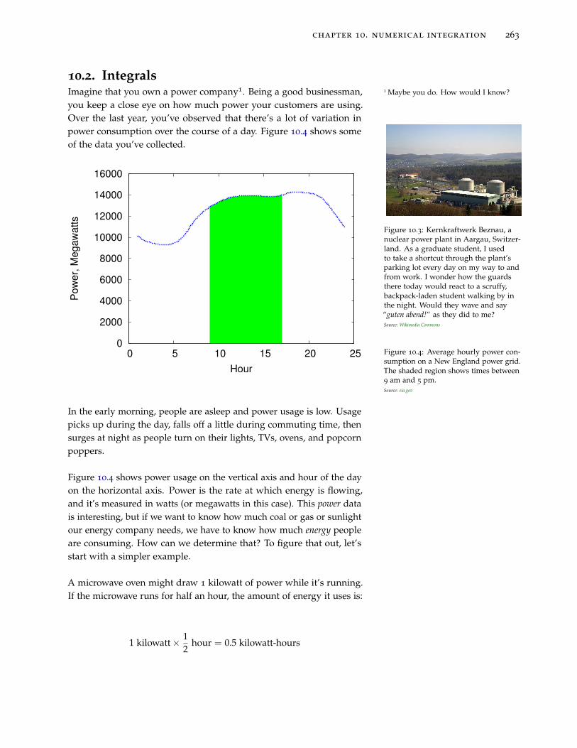
10.2. IntegralsImagine that you own a power company1. Being a good businessman, 1 Maybe you do. How would I know?

you keep a close eye on how much power your customers are using.

Over the last year, you’ve observed that there’s a lot of variation in

power consumption over the course of a day. Figure 10.4 shows some

of the data you’ve collected.

Figure 10.3: Kernkraftwerk Beznau, anuclear power plant in Aargau, Switzer-land. As a graduate student, I usedto take a shortcut through the plant’sparking lot every day on my way to andfrom work. I wonder how the guardsthere today would react to a scruffy,backpack-laden student walking by inthe night. Would they wave and say“guten abend!” as they did to me?Source: Wikimedia Commons

0

2000

4000

6000

8000

10000

12000

14000

16000

0 5 10 15 20 25

Po

we

r, M

eg

aw

att

s

Hour

Figure 10.4: Average hourly power con-sumption on a New England power grid.The shaded region shows times between9 am and 5 pm.Source: eia.gov

In the early morning, people are asleep and power usage is low. Usage

picks up during the day, falls off a little during commuting time, then

surges at night as people turn on their lights, TVs, ovens, and popcorn

poppers.

Figure 10.4 shows power usage on the vertical axis and hour of the day

on the horizontal axis. Power is the rate at which energy is flowing,

and it’s measured in watts (or megawatts in this case). This power data

is interesting, but if we want to know how much coal or gas or sunlight

our energy company needs, we have to know how much energy people

are consuming. How can we determine that? To figure that out, let’s

start with a simpler example.

A microwave oven might draw 1 kilowatt of power while it’s running.

If the microwave runs for half an hour, the amount of energy it uses is:

1 kilowatt ×1

2hour = 0.5 kilowatt-hours

https://commons.wikimedia.org/wiki/File:Kkw_beznau.jpg

http://www.eia.gov/todayinenergy/detail.cfm?id=4190

264 practical computing for science and engineering

Kilowatt-hours is a unit of energy. When we do the calculation above,

it’s equivalent to determining the shaded area shown in Figure 10.5.

Mathematically, we could express it like this:

E = P(t)∆t

where E is energy, P(t) = 1000 watts (a steady, unvarying power con-

sumption), and ∆t is the amount of time the microwave oven is running.

0

200

400

600

800

1000

-0.1 0 0.1 0.2 0.3 0.4 0.5 0.6

Po

we

r, in

Wa

tts

Time, in Hours

Figure 10.5: If we assume that the mi-crowave oven uses a constant amountof power while it’s running, the energyit consumes is equal to the shaded areain this graph, which is the power (P, inwatts) multiplied by the amount of time(∆t, in hours).

Unfortunately for our power company, Figure 10.4 shows that our

customers don’t use the same amount of power all the time, so we

can’t just do a simple multiplication to find out how much energy they

use. If we want to know how much energy is used between 9 am and

5pm, we need to determine the size of the shaded area in Figure 10.4.

Mathematically, that’s equivalent to evaluating the following integral

equation:

E =∫ 5pm

9amP(t)dt

Figure 10.6: Scottish inventor andentrepreneur James Watt, most famousfor the invention of the steam engine,for whom the unit of power is named.Source: Wikimedia Commons

The important thing to remember is that the integral is just the area un-

der the curve defined by the P(t) function. As we saw in the microwave

oven example, this is sometimes trivial to calculate. In calculus class

we learn some mathematical tricks to evaluate the integrals of more

complicated functions.

https://commons.wikimedia.org/wiki/File:Bust_of_James_Watt.JPG


In the following, we’ll see how to use a computer program to estimate

the value of such integrals without using any tricks. To do so, we’ll

combine a little modern computing power with the basic principles

that Newton and Leibniz used when they invented calculus way back

in the 1600s.

The integral here is called a “definiteintegral” because it only covers a rangebetween two limits (9 am and 5 pmin this case). The techniques we’lltalk about in this chapter are all forfinding approximate values for definiteintegrals.

10.3. Slicing up the ProblemIf Newton and Leibniz had been familiar with microwave ovens and

power plants, they’d have approached the problem this way: slice up

the area into manageable bits.

Figure 10.7: We can slice a functionup so that each slice is approximatelyrectangular.Source: Wikimedia Commons

The inventors of calculus realized that the area under a curve could be

approximated by the total area of a row of rectangles, as in Figure 10.8,

like slices from a loaf of bread. As in the microwave oven example, the

area of each rectangle is easy to calculate.

0.9

1

1.1

1.2

1.3

1.4

1.5

-2 -1 0 1 2 3 4

Figure 10.8: The area under the smoothcurve is approximately the same as thetotal area of a row of rectangles of variousheights.

0.9

1

1.1

1.2

1.3

1.4

1.5

-2 -1 0 1 2 3 4

0.9

1

1.1

1.2

1.3

1.4

1.5

-2 -1 0 1 2 3 4

Figure 10.9: More slices give a betterapproximation.

If we want a better approximation, we can just use thinner slices, as

in Figure 10.9. Mathematicians have found that in some cases we can

arrive at the exact area under the curve by mathematically determining

what the area would be if the width of the slices went to zero. Sometimes

we can’t calculate this limit, though. In those cases, we have to be

satisfied with an approximation, but that’s not so bad, because we can

often make our approximation as accurate as we want by choosing the

width of our slices.

https://commons.wikimedia.org/wiki/File:Vegan_no-knead_whole_wheat_bread_loaf,_sliced,_September_2010.jpg


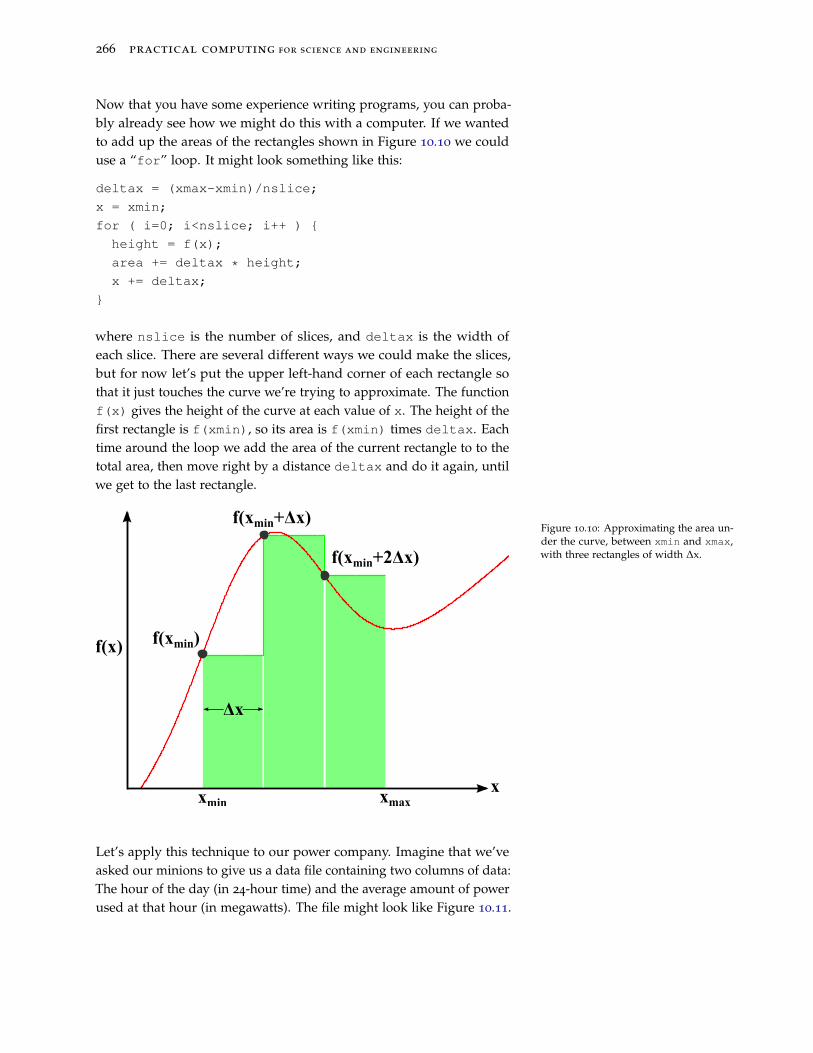
Now that you have some experience writing programs, you can proba-

bly already see how we might do this with a computer. If we wanted

to add up the areas of the rectangles shown in Figure 10.10 we could

use a “for” loop. It might look something like this:

deltax = (xmax-xmin)/nslice;

x = xmin;

for ( i=0; i<nslice; i++ ) {

height = f(x);

area += deltax * height;

x += deltax;

}

where nslice is the number of slices, and deltax is the width of

each slice. There are several different ways we could make the slices,

but for now let’s put the upper left-hand corner of each rectangle so

that it just touches the curve we’re trying to approximate. The function

f(x) gives the height of the curve at each value of x. The height of the

first rectangle is f(xmin), so its area is f(xmin) times deltax. Each

time around the loop we add the area of the current rectangle to to the

total area, then move right by a distance deltax and do it again, until

we get to the last rectangle.

xmin

Δx

f(xmin+Δx)

f(xmin)

f(xmin+2Δx)

x

f(x)

xmax

Figure 10.10: Approximating the area un-der the curve, between xmin and xmax,with three rectangles of width ∆x.

Let’s apply this technique to our power company. Imagine that we’ve

asked our minions to give us a data file containing two columns of data:

The hour of the day (in 24-hour time) and the average amount of power

used at that hour (in megawatts). The file might look like Figure 10.11.


Program 10.1 is designed to read this file and estimate the area under

the power curve between 9 am and 5 pm. Notice that we’ve placed the

slices as shown in Figure 10.10, which means that each rectangle starts

on the hour and covers the time until the next hour begins. This means

that we don’t want to include the 5:00 measurement (hour 17) in the

total area, since we’re assuming that this measurement is an estimate

of the power used between 5 pm and 6 pm, which is outside the range

we’re interested in. (See Section 10.5 for more about this.)

Figure 10.11: The contents of thefile “power.dat”, containing hourlypower measurements from our powercompany:

1 10110.66

2 9636.32

3 9376.79

4 9283.72

5 9433.38

6 10025.68

7 11181.30

8 12193.26

9 12855.83

10 13332.67

11 13685.37

12 13871.35

13 13918.52

14 13935.75

15 13867.86

16 13833.21

17 13976.59

18 14238.24

19 14253.39

20 14163.90

21 13948.21

22 13220.34

23 12059.76

24 10920.85

Also notice that, even though each slice has a width of 1 hour, the

program goes ahead and explicitly multiplies by this width, just to

make it clear that we’re calculating the area of the rectangular slice by

multiplying its height times its width. If our data were at half-hour

intervals, we’d change the 1.0 to 0.5.

Program 10.1: power.cpp

#include <stdio.h>

int main () {

int hour[24];

double power[24];

FILE *input;

int i;

double area=0.0;

input = fopen("power.dat","r");

for ( i=0; i<24; i++ ) {

fscanf( input, "%d", &hour[i] );

fscanf( input, "%lf", &power[i] );

}

fclose ( input );

for ( i=0; i<24; i++ ) {

// Don't include the 5pm hour:

if ( hour[i] >= 9 && hour[i] < 17 ) {

area += power[i] * 1.0; // 1 hour.

}

}

printf ( "Total energy from 9am-5pm is %lf Mw-hours\n", area );

}

Exercise 48: Power to the People!

Using nano, create the file power.dat by entering the data


from Figure 10.11. Create, compile and run Program 10.1.

Make a note of the result, for later use.

By looking at Figure 10.4, make a rough estimate of the 9

to 5 power usage by multiplying the curve’s approximate

height, in megawatts, by 8 hours (the interval between 9 am

and 5 pm). Is your rough estimate consistent with Program

10.1’s estimate?

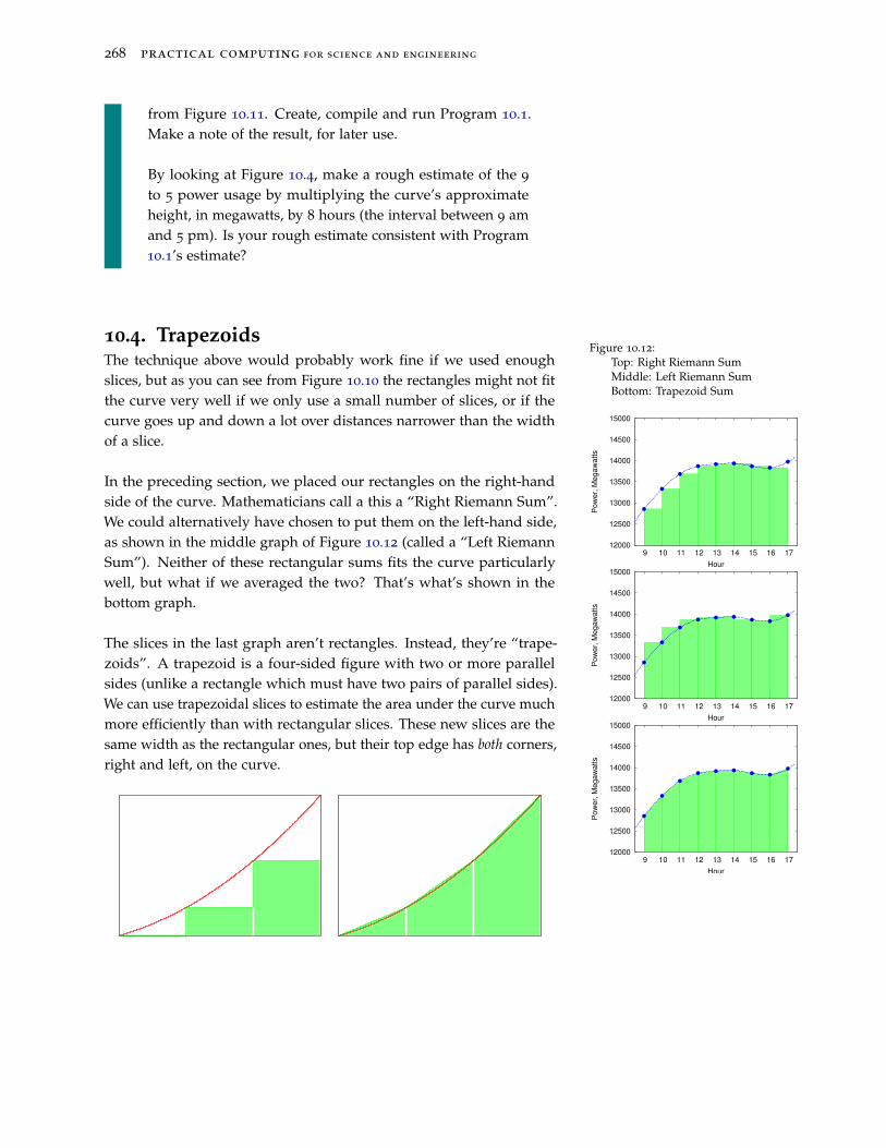
10.4. TrapezoidsThe technique above would probably work fine if we used enough

slices, but as you can see from Figure 10.10 the rectangles might not fit

the curve very well if we only use a small number of slices, or if the

curve goes up and down a lot over distances narrower than the width

of a slice.

In the preceding section, we placed our rectangles on the right-hand

side of the curve. Mathematicians call a this a “Right Riemann Sum”.

We could alternatively have chosen to put them on the left-hand side,

as shown in the middle graph of Figure 10.12 (called a “Left Riemann

Sum”). Neither of these rectangular sums fits the curve particularly

well, but what if we averaged the two? That’s what’s shown in the

bottom graph.

Figure 10.12:Top: Right Riemann SumMiddle: Left Riemann SumBottom: Trapezoid Sum

12000

12500

13000

13500

14000

14500

15000

9 10 11 12 13 14 15 16 17

Po

we

r, M

eg

aw

att

s

Hour

12000

12500

13000

13500

14000

14500

15000

9 10 11 12 13 14 15 16 17

Po

we

r, M

eg

aw

att

s

Hour

12000

12500

13000

13500

14000

14500

15000

9 10 11 12 13 14 15 16 17

Po

we

r, M

eg

aw

att

s

Hour

The slices in the last graph aren’t rectangles. Instead, they’re “trape-

zoids”. A trapezoid is a four-sided figure with two or more parallel

sides (unlike a rectangle which must have two pairs of parallel sides).

We can use trapezoidal slices to estimate the area under the curve much

more efficiently than with rectangular slices. These new slices are the

same width as the rectangular ones, but their top edge has both corners,

right and left, on the curve.


xmin

Δx

f(xmin+Δx)

f(xmin)

f(xmin+2Δx)

x

f(x)

xmax

f(xmin+3Δx)

Figure 10.13: Approximating the area un-der the curve, between xmin and xmax,with three trapezoids of width ∆x. Com-pare this with Figure 10.10, which usesrectangles.

Figure 10.13 shows how we might slice up an area into trapezoidal

sections. As before, we can add up the areas of the slices to get an

estimate of the area under the curve, but to do this we’ll first need to

know how to find the area of a trapezoid.

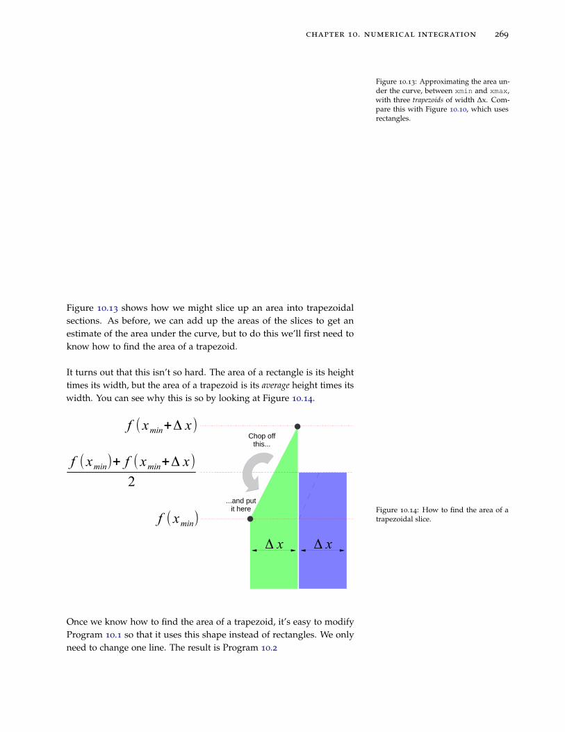
It turns out that this isn’t so hard. The area of a rectangle is its height

times its width, but the area of a trapezoid is its average height times its

width. You can see why this is so by looking at Figure 10.14.

f (xmin+Δ x)

f (xmin)

f (xmin)+ f (xmin+Δ x)

2

Chop offthis...

...and putit here

Δ x Δ x

Figure 10.14: How to find the area of atrapezoidal slice.

Once we know how to find the area of a trapezoid, it’s easy to modify

Program 10.1 so that it uses this shape instead of rectangles. We only

need to change one line. The result is Program 10.2


Program 10.2: power.cpp, with trapezoids instead of rectangles

#include <stdio.h>

int main () {

int hour[24];

double power[24];

FILE *input;

int i;

double area=0.0;

input = fopen("power.dat","r");

for ( i=0; i<24; i++ ) {

fscanf( input, "%d", &hour[i] );

fscanf( input, "%lf", &power[i] );

}

fclose ( input );

for ( i=0; i<24; i++ ) {

// Don't include the 5pm hour:

if ( hour[i] >= 9 && hour[i] < 17 ) {

area += 0.5 * (power[i] + power[i+1]) * 1.0; // 1 hour.

}

}

printf ( "Total energy from 9am-5pm is %lf Mw-hours\n", area );

}

Figure 10.15: The hammer dulcimer hasa trapezoidal shape. The American folkband “Trapezoid” took its name fromthe shape of this instrument.Source: Wikimedia Commons

Program 10.2 multiplies the width of each trapezoid by its average

height. The average height is:

power[i]+ power[i+1]

2

This way of approximating the value of an integral is called the “trape-

zoid rule”.

Exercise 49: More Power to You!

Modify your power.cpp program so that it looks like Pro-

gram 10.2. Compile and run it. How does the result compare

with the result from the previous version? Does this agree

with what you’d expect after looking at Figure 10.12?

https://commons.wikimedia.org/wiki/File:Oprekelj_-_ugla%C5%A1evanje.jpg


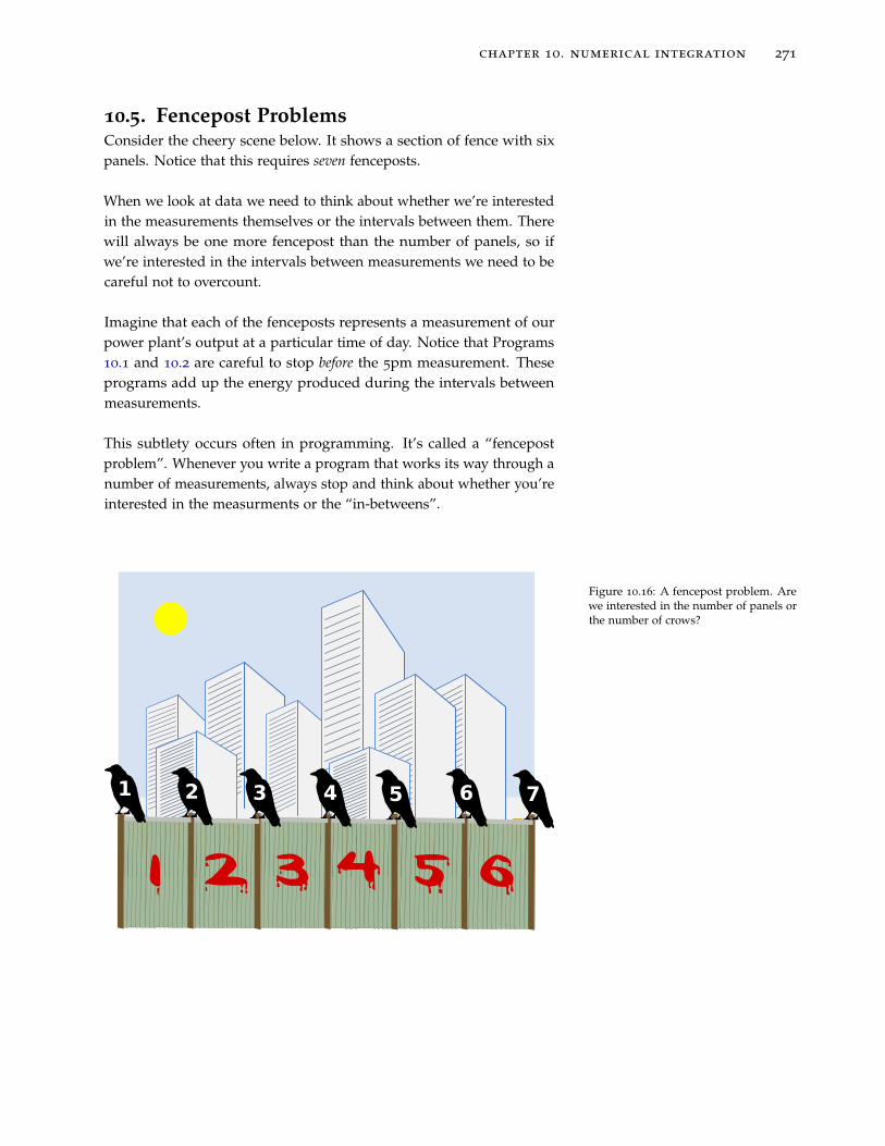
10.5. Fencepost ProblemsConsider the cheery scene below. It shows a section of fence with six

panels. Notice that this requires seven fenceposts.

When we look at data we need to think about whether we’re interested

in the measurements themselves or the intervals between them. There

will always be one more fencepost than the number of panels, so if

we’re interested in the intervals between measurements we need to be

careful not to overcount.

Imagine that each of the fenceposts represents a measurement of our

power plant’s output at a particular time of day. Notice that Programs

10.1 and 10.2 are careful to stop before the 5pm measurement. These

programs add up the energy produced during the intervals between

measurements.

This subtlety occurs often in programming. It’s called a “fencepost

problem”. Whenever you write a program that works its way through a

number of measurements, always stop and think about whether you’re

interested in the measurments or the “in-betweens”.

Figure 10.16: A fencepost problem. Arewe interested in the number of panels orthe number of crows?


10.6. Uneven SlicesIn the preceding examples we’ve assumed that our measurements were

evenly spaced. What if they’re not, though? To explore that possibility,

let’s take a road trip!

Figure 10.17: In October 1925 Harry Lil-lis “Bing” Crosby and his pal Al Rinkerset out from Spokane, Washington,bound for Los Angeles in Al’s beat-upFord Model T. Over the next threeweeks they made their way down thecoast, stopping whenever the car brokedown and working a day or two to earnsome money. The car survived up tothe outskirts of LA, where its enginefinally died. They were taken in by Al’ssister, the singer Mildred Bailey, whohelped the boys find jobs performingin LA. Within a year they were hiredby internationally-known bandleaderPaul Whiteman. The rest, as they say, ishistory.Source: Wikimedia Commons

Your car’s odometer tells you how far you’ve driven, but modern cars

don’t measure distance directly. Instead, they use your velocity and a

little bit of calculus to determine how many miles you’ve gone.

A mathematician would say that velocity is the time derivative of

position, and she might write that relationship like this:

v =dx

dt

where dx represents a small change in position, dt is a small change in

time, and v is the velocity. If the velocity doesn’t change, then this is

the same as saying that velocity is equal to distance divided by time.

If we know the velocity and the time, we can calculate the distance as

distance = velocity × time.

If the velocity isn’t constant, things get more complicated. In that case,

our mathematician friend would tell us that we could find the distance

like this:

distance =∫ t1

t0

v(t)dt

where v(t) is a function that tells us the velocity at a given time. The

times t0 and t1 are when our trip starts and ends, repectively.

That looks complicated, but it’s just like what we’ve been doing earlier

in this chapter. If we’re given some data about the car’s velocity at

various times, we can write a computer program to do the integral

above and estimate the distance we’ve traveled.

Imagine we’re going on a long trip. When we start, our velocity is

zero. Then we pull out onto the highway and start driving. We can’t

drive at a constant speed, though. Sometimes traffic will slow us down.

Sometimes we’ll be driving on roads with higher or lower speed limits.

Sometimes we’ll be zoned out listening to our favorite tunes and find

that we’ve spent the last ten miles drifting along behind a spluttering

jalopy. Eventually, we’ll reach our destination and our velocity will go

back to zero again.

If we noted the time and our speed occasionally, the data might look

like the large dots in Figure 10.18. We’re lazy and easily distracted, so

we haven’t done the measurements at regular intervals.

https://commons.wikimedia.org/wiki/File:The_Rhythm_Boys_-_Radio_Mirror,_October_1943.jpg


0

10

20

30

40

50

60

70

80

90

0 1 2 3 4 5 6 7

Sp

ee

d,

MP

H

Time, Hours

Figure 10.18: The large dots representmeasurements of our speed. If we couldhave constantly monitored the speed itmight have looked like the dashed curve.The whole trip takes about six and a halfhours.

As you can see from the figure, we can draw trapezoids that connect

the dots, just as we did with the power plant data. The only difference

is that these trapezoids aren’t all the same width. That’s not a problem.

We just need to take the width into account when we calculate the area

of each trapezoid. Adding all of the areas together gives us the total

area of the shaded region in Figure 10.18. The size of this shaded area

is approximately equal to the distance we’ve traveled, as given by the

integral equation our mathematician friend gave us above.

0.0 0.0

0.5 46.7

0.8 62.1

0.9 70.1

1.5 74.1

1.7 69.3

1.9 74.8

2.1 78.9

3.2 76.8

4.0 73.9

4.5 60.9

4.8 65.6

4.9 58.1

6.0 64.3

6.3 37.1

6.5 0.0

Figure 10.19: The file roadtrip.dat,used by Program 10.3. The first columnis time, in hours. The second columnis our speed, in miles per hour, at thattime.

Program 10.3 does the work for us. It’s similar to Program 10.2, but

it doesn’t assume that there’s a particular number of measurements.

The power plant program knew that there were 24 hours in a day, so it

could assume there would be 24 measurements to read from its data

file. On our road trip we just took some measurements at random times.

On the next trip we might take more or fewer. Because of this, the new

program doesn’t start by reading all of the data into a fixed-size array.

Instead, it uses a different strategy that just focuses on measurements

one or two at a time, as they’re read from the data file.

For each of the trapezoids in Figure 10.18 we need two pairs of time

and speed measurements2. The difference in the two times tells us 2 See Section 10.5.

the width of the trapezoid. The average of the two speeds tells us the

average height of the trapezoid. Program 10.3 waits until it has read

the first two lines from the data file, then does these calculations to find

the area of the first trapezoid. Then it continues on, doing the same for

each subsequent pair of data points. Notice that, at any point in our


trip, the area we’ve accumulated so far will be equal to the distance

we’ve traveled so far. To emphasize this, the program prints out the

updated time and distance each time it reads a new data point from

the file.

Program 10.3: roadtrip.cpp

#include <stdio.h>

int main () {

double hour, velocity;

double oldhour, oldvelocity;

double height, width;

double area=0.0;

int nmeasurements=0;

FILE *input;

input = fopen("roadtrip.dat","r");

while ( fscanf( input, "%lf %lf", &hour, &velocity ) != EOF ) {

if ( nmeasurements != 0 ) {

height = 0.5 * (oldvelocity+velocity);

width = hour - oldhour;

area += height*width;

printf ( "Distance after %lf hours is %lf miles\n",

hour, area );

}

oldhour = hour;

oldvelocity = velocity;

nmeasurements++;

}

fclose ( input );

printf ( "Total distance is %lf miles\n", area );

}

Notice that the program uses two variables, oldhour and oldvelocity,

to remember the previous data point’s values. To make the program

wait until there are at least two data points, we use the variable

nmeasurements to count the number of points we’ve read so far,

and test this value before we start doing any calculations. After the first

trip around the loop, oldhour and oldvelocity have been set and

we’re ready to calculate the area of the first trapezoid during the next

trip around the loop.

Remember that our result is only an estimate of the distance we’ve

traveled. The estimate would be more accurate if we recorded more

speed measurements during our trip. (If we’d only written down the

speed at the beginning and end of the trip, the program would tell us

that the distance was zero!)


10.7. Integrating FunctionsIn the exercises above, we’ve been finding the integral of a curve defined

by data points, instead of being defined by some mathematical function.

This is one common reason people use numerical integration: they have

some data points, but don’t know the underlying mathematics that

generated them. You can’t use calculus to compute the integral of a

function if you don’t know what that function is!

But what if you do know the function? As noted before, integration can

be hard, and much of what we learn in calculus class is a set of tricks

for finding the values of certain integrals. Sometimes, though, there

are no applicable tricks that will let write down a value for a particular

integral in terms of elementary functions (trigonometric functions,

logarithms, etc.), or even “special” functions (the error function, the

gamma function, etc.). Integrals of some seemingly simple expressions

like sin(sin(x)) turn out to be impossible to evaluate.

-1

-0.5

0

0.5

1

0 1 2 3 4 5 6

sin

(x)

x

x=π

Area ofInterest

Figure 10.20: sin(x)

Happily, in these cases the poor beleaguered mathematician can turn

to numerical integration. As long as we can find the value of a function

at any point within the range we’re interested in, we can numerically

approximate the value of the definite integral of the function over that

range.

Let’s look at an example where we can find the value of the integral

mathematically. That will allow us to compare an exact mathematical

solution to an approximate solution computed by the trapezoid rule.

0

0.2

0.4

0.6

0.8

1

0 0.5 1 1.5 2 2.5 3

sin

(x)

x

True Area = 2.0

0

0.2

0.4

0.6

0.8

1

0 0.5 1 1.5 2 2.5 3

sin

(x)

x

Figure 10.21: The integral of the sinefunction between 0 and π has a valueof 2 (the area under the curve in the topgraph). The bottom graph shows thisarea approximated by five trapezoidalslices.

For example, in calculus class we learned how to integrate the sine

function (see Figure 10.20):

∫ B

Asin(x)dx = cos(A)− cos(B)

This tells us that the area under the sine curve between 0 and π is

exactly cos(0)− cos(π) = 2, as shown in the top graph of Figure 10.21.

Let’s use the trapezoid rule to find this same area, and see how close it

gets to the true answer.

That’s what Program 10.4 does. Notice that, instead of using sin(x)

directly, the program uses a function we define ourselves, named func.

If we ever want to use this program to integrate something other than

sin(x), we’ll only need to change this function definition. We can put

anything we want to inside func. It could be as simple as sin(x) or

as complicated as the “Red Baron” flight path we used in Chapter 9.


Program 10.4: integrate.cpp

#include <stdio.h>

#include <math.h>

double func( double x ) {

double value;

value = sin(x);

return(value);

}

int main () {

double x, delta, area=0;

double height;

double xmin=0.0, xmax=M_PI;

int i, nsteps=5;

delta = (xmax-xmin)/nsteps;

x = xmin;

for ( i=0; i<nsteps; i++ ) {

height = ( func(x) + func(x+delta) ) / 2.0;

area += delta * height;

x += delta;

}

printf ( "Integral from %lf to %lf is %lf\n",

xmin, xmax, area );

}

Figure 10.22: Slicing an onion in prepa-ration for integrating it into dinner.Source: Wikimedia Commons

The program specifies how many slices we want to use by setting the

value of nsteps. (It’s set to 5 here.) The variables xmin and xmax

set the range over which we want to integrate. Notice that we use the

symbol M_PI from math.h to set xmax, so we don’t have to type out a

long string of π’s digits.

Most of the program’s work is done in the “for” loop that works its

way through the slices, one at a time, adding each area to the total area.

As we go through the slices, we need to keep track of where we are

on the x axis. Before we start the “for” loop, we set the value of x

to xmin, and then we add the slice width (delta) to this when we’re

ready to go to the next slice.

To find the area of each slice, we multiply its average height by its

width (delta). See Figures 10.13 and 10.14.

https://commons.wikimedia.org/wiki/File:Matlagning_(2).jpg


Exercise 50: Sines of the Times

1. Create, compile, and run Program 10.4. How close does

its approximation come to the true value of the area?

2. Now change nsteps to 10, recompile, and run again. Is

the answer closer to the true value? Try nsteps values

of 100 and 1000. Does the program take noticeably longer

if you use these large values for nsteps?

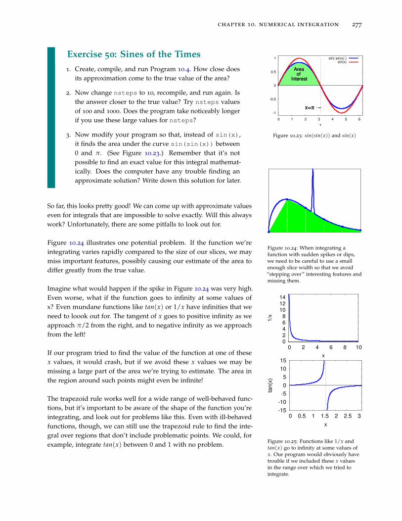
3. Now modify your program so that, instead of sin(x),

it finds the area under the curve sin(sin(x)) between

0 and π. (See Figure 10.23.) Remember that it’s not

possible to find an exact value for this integral mathemat-

ically. Does the computer have any trouble finding an

approximate solution? Write down this solution for later.

-1

-0.5

0

0.5

1

0 1 2 3 4 5 6

x

x=πx=π

sin( sin(x) )sin(x)

Area ofInterest

Area ofInterest

Figure 10.23: sin(sin(x)) and sin(x)

So far, this looks pretty good! We can come up with approximate values

even for integrals that are impossible to solve exactly. Will this always

work? Unfortunately, there are some pitfalls to look out for.

Figure 10.24 illustrates one potential problem. If the function we’re

integrating varies rapidly compared to the size of our slices, we may

miss important features, possibly causing our estimate of the area to

differ greatly from the true value.

Figure 10.24: When integrating afunction with sudden spikes or dips,we need to be careful to use a smallenough slice width so that we avoid“stepping over” interesting features andmissing them.

Imagine what would happen if the spike in Figure 10.24 was very high.

Even worse, what if the function goes to infinity at some values of

x? Even mundane functions like tan(x) or 1/x have infinities that we

need to loook out for. The tangent of x goes to positive infinity as we

approach π/2 from the right, and to negative infinity as we approach

from the left!

If our program tried to find the value of the function at one of these

x values, it would crash, but if we avoid these x values we may be

missing a large part of the area we’re trying to estimate. The area in

the region around such points might even be infinite!

0 2 4 6 8

10 12 14

0 2 4 6 8 10

1/x

x

-15

-10

-5

0

5

10

15

0 0.5 1 1.5 2 2.5 3

tan(x

)

x

Figure 10.25: Functions like 1/x andtan(x) go to infinity at some values ofx. Our program would obviously havetrouble if we included these x valuesin the range over which we tried tointegrate.

The trapezoid rule works well for a wide range of well-behaved func-

tions, but it’s important to be aware of the shape of the function you’re

integrating, and look out for problems like this. Even with ill-behaved

functions, though, we can still use the trapezoid rule to find the inte-

gral over regions that don’t include problematic points. We could, for

example, integrate tan(x) between 0 and 1 with no problem.


But what about. . . ?

Wait a minute. Doesn’t Program 10.4 calculate func(x) for the same values of x multiple times?

Take a look at Figure 10.13 again. If Program 10.4 were calculating the area of the first slice it would use

func(xmin) for the height of the trapezoid’s left-hand side and func(xmin+delta) for the right-hand

side. For the second slice, it would use func(xmin+delta) for the left and func(xmin+2*delta)

for the right. On the third slice the program would use func(xmin+2*delta) for the left and

func(xmin+3*delta) for the right.

It takes the computer some time to process the statements inside a function. The program would run

faster if we didn’t have to calculate each of the middle func values twice. If func were more complicated,

or if we had a lot of slices, the amount of time saved could be large.

We can do a little algebra and eliminate the duplication. If we have n slices we could write the sum of

their areas like this:

A = ∆xf (xmin) + f (xmin + ∆x)

2+

∆xf (xmin + ∆x) + f (xmin + 2∆x)

2+ ... +

∆xf (xmin + (n − 1)∆x) + f (xmax)

2

Collecting terms, we can rewrite the equation like this, so that we only calculate the value of f (x) once

for each value of x:

A = ∆x

[

f (xmin) + f (xmax)

2+

n−1

∑i=1

f (xmin + i∆x)

]

To take advantage of this, we could replace the loop in Program 10.4 with a loop like this:

double sum = 0;

...


sum += func(x+delta);

x += delta;

}

area = delta*( (func(xmin) + func(xmax))/2.0 + sum );

There! We fixed it.


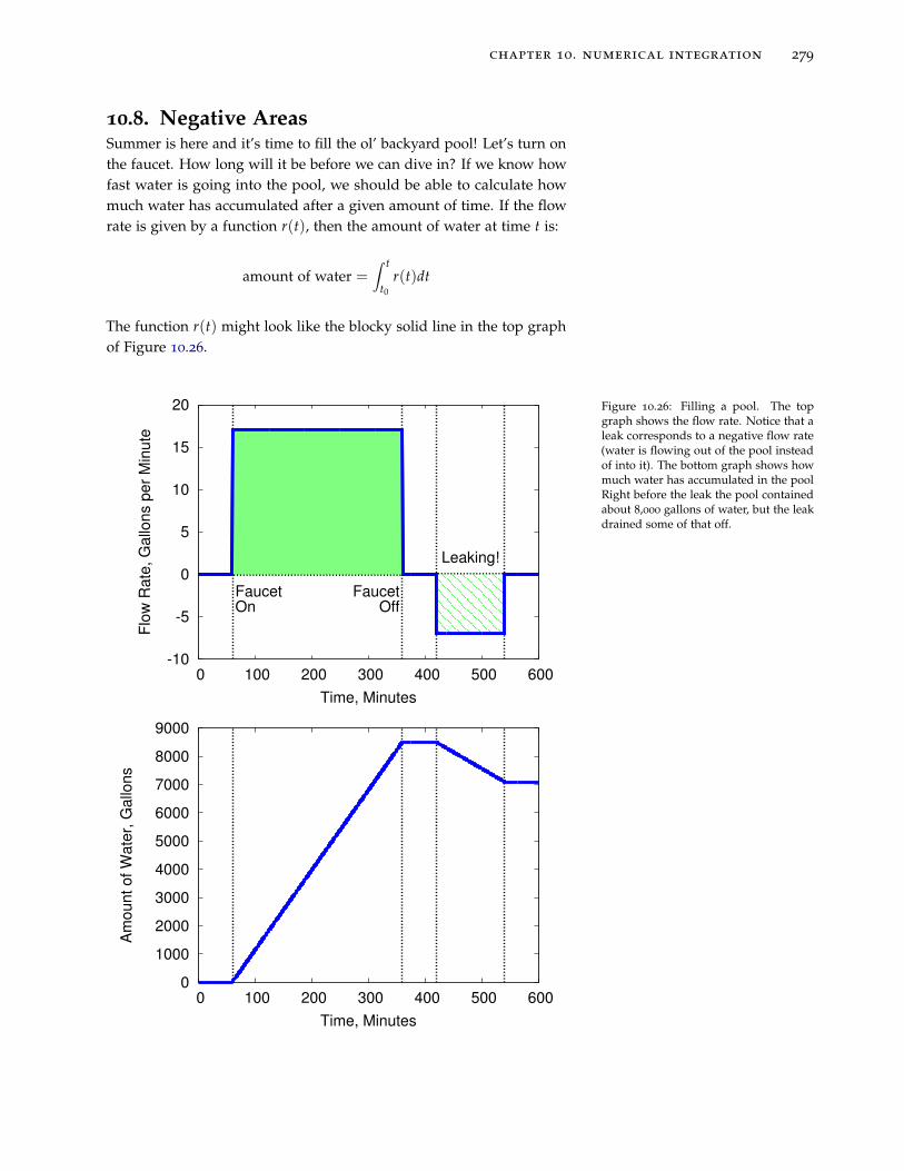
10.8. Negative AreasSummer is here and it’s time to fill the ol’ backyard pool! Let’s turn on

the faucet. How long will it be before we can dive in? If we know how

fast water is going into the pool, we should be able to calculate how

much water has accumulated after a given amount of time. If the flow

rate is given by a function r(t), then the amount of water at time t is:

amount of water =∫ t

t0

r(t)dt

The function r(t) might look like the blocky solid line in the top graph

of Figure 10.26.

-10

-5

0

5

10

15

20

0 100 200 300 400 500 600

Flo

w R

ate

, G

allo

ns p

er

Min

ute

Time, Minutes

FaucetOn

FaucetOff

Leaking!

0

1000

2000

3000

4000

5000

6000

7000

8000

9000

0 100 200 300 400 500 600

Am

ount of W

ate

r, G

allo

ns

Time, Minutes

Figure 10.26: Filling a pool. The topgraph shows the flow rate. Notice that aleak corresponds to a negative flow rate(water is flowing out of the pool insteadof into it). The bottom graph shows howmuch water has accumulated in the poolRight before the leak the pool containedabout 8,000 gallons of water, but the leakdrained some of that off.


The amount of water in the pool is given by the integral of this curve,

which is just the shaded area between the curve and the x axis in the

top graph of Figure 10.26.

This figure shows the pool being filled for a while at a constant rate of

17 gallons per minute. Eventually, we accumulate about 8,000 gallons

of water, as shown in the bottom graph, which shows the integral of

r(t) up to a given time.

Uh oh! after filling the pool, it sprang a leak! This let water run out of

the pool at a rate of 7 gallons per minute until we found the leak and

patched it. If r(t) is the rate of water going into the pool, that means

that r(t) had a negative value while the pool was leaking, as shown in

the top graph of Figure 10.26.

If we used a computer program to slice up this curve and calculate its

area, we’d find that the leak would contribute a negative amount to the

sum because the height of the slices in this region would be negative.

This is actually what we expect: The first part of the curve shows water

flowing into the pool, and the second part of the curve shows water

flowing out. To find out how much water we have at the end, we need

to subtract the water that escaped through the leak.

The important thing to know is that we don’t have to modify our

programs in any way because of this. It just gets taken care of automat-

ically when we multiply the height of a slice times its width. When

the function we’re integrating has a negative value, it contributes a

negative amount to the total area.


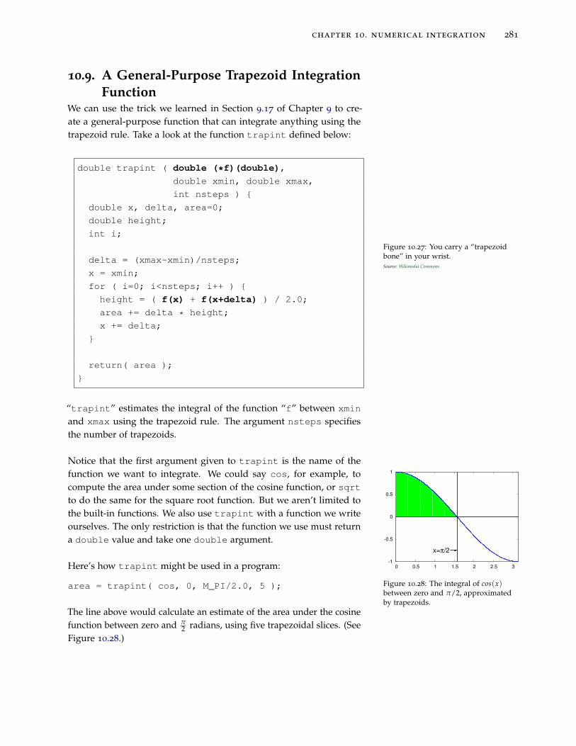
10.9. A General-Purpose Trapezoid Integration

FunctionWe can use the trick we learned in Section 9.17 of Chapter 9 to cre-

ate a general-purpose function that can integrate anything using the

trapezoid rule. Take a look at the function trapint defined below:

Figure 10.27: You carry a “trapezoidbone” in your wrist.Source: Wikimedia Commons

double trapint ( double (*f)(double),

double xmin, double xmax,

int nsteps ) {

double x, delta, area=0;

double height;

int i;

delta = (xmax-xmin)/nsteps;

x = xmin;


height = ( f(x) + f(x+delta) ) / 2.0;

area += delta * height;

x += delta;

}

return( area );

}

“trapint” estimates the integral of the function “f” between xmin

and xmax using the trapezoid rule. The argument nsteps specifies

the number of trapezoids.

Notice that the first argument given to trapint is the name of the

function we want to integrate. We could say cos, for example, to

compute the area under some section of the cosine function, or sqrt

to do the same for the square root function. But we aren’t limited to

the built-in functions. We also use trapint with a function we write

ourselves. The only restriction is that the function we use must return

a double value and take one double argument.

-1

-0.5

0

0.5

1

0 0.5 1 1.5 2 2.5 3

x=π/2

Figure 10.28: The integral of cos(x)between zero and π/2, approximatedby trapezoids.

Here’s how trapint might be used in a program:

area = trapint( cos, 0, M_PI/2.0, 5 );

The line above would calculate an estimate of the area under the cosine

function between zero and π

2 radians, using five trapezoidal slices. (See

Figure 10.28.)

https://commons.wikimedia.org/wiki/File:Carpus.svg


Figure 10.29:Thomas Simpson, 1710-1761.Source: University of St. Andrews

But what about. . . ?

Are trapezoids the best possible shape for numerical integration?

Not necessarily. There are other techniques that work better in

some circumstances. Sometimes these techniques will give a more

accurate estimate of the area. Sometimes they’ll give you an esti-

mate more quickly.

One common alternative to the “trapezoid rule” is called “Simp-

son’s rule”, named after 18th-Century British mathematician

Thomas Simpson. Instead of connecting two data points with

a straight line to make the top of each slice, Simpson’s rule draws

a section of a parabola through three adjacent points.

16

17

18

19

20

21

0.8 1 1.2 1.4 1.6 1.8 2 2.2

In the graph above, the dashed line represents a section of a

parabola that approximates the shape of the curve. This parabola

forms the top of slice. As you can see, Simpson’s rule often fits a

curve better than the trapezoid rule. The area of the slice can be

determined from the parameters of this parabola and the width of

the slice.

There are many other numerical integration schemes. One of them

is the Monte Carlo method we’ll talk about in a later section of this

chapter. It doesn’t use slices at all!

http://www-history.mcs.st-andrews.ac.uk/PictDisplay/Simpson.html


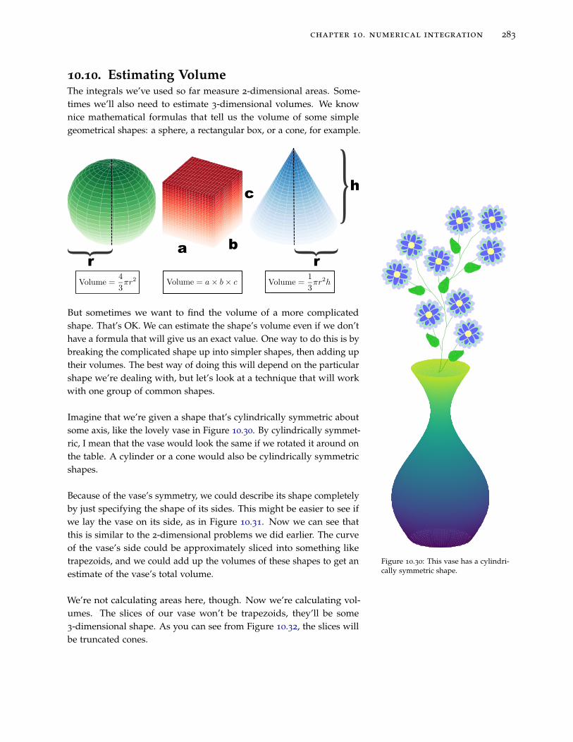
10.10. Estimating VolumeThe integrals we’ve used so far measure 2-dimensional areas. Some-

times we’ll also need to estimate 3-dimensional volumes. We know

nice mathematical formulas that tell us the volume of some simple

geometrical shapes: a sphere, a rectangular box, or a cone, for example.

But sometimes we want to find the volume of a more complicated

shape. That’s OK. We can estimate the shape’s volume even if we don’t

have a formula that will give us an exact value. One way to do this is by

breaking the complicated shape up into simpler shapes, then adding up

their volumes. The best way of doing this will depend on the particular

shape we’re dealing with, but let’s look at a technique that will work

with one group of common shapes.

Figure 10.30: This vase has a cylindri-cally symmetric shape.

Imagine that we’re given a shape that’s cylindrically symmetric about

some axis, like the lovely vase in Figure 10.30. By cylindrically symmet-

ric, I mean that the vase would look the same if we rotated it around on

the table. A cylinder or a cone would also be cylindrically symmetric

shapes.

Because of the vase’s symmetry, we could describe its shape completely

by just specifying the shape of its sides. This might be easier to see if

we lay the vase on its side, as in Figure 10.31. Now we can see that

this is similar to the 2-dimensional problems we did earlier. The curve

of the vase’s side could be approximately sliced into something like

trapezoids, and we could add up the volumes of these shapes to get an

estimate of the vase’s total volume.

We’re not calculating areas here, though. Now we’re calculating vol-

umes. The slices of our vase won’t be trapezoids, they’ll be some

3-dimensional shape. As you can see from Figure 10.32, the slices will

be truncated cones.


-2.5

-2

-1.5

-1

-0.5

0

0.5

1

1.5

2

2.5

1 2 3 4 5 6

y

x

Figure 10.31: We can graph the curvesthat define the shape of the vase, andapproximate them with simpler shapes.

Figure 10.32: The vase’s volume couldbe sliced into a bunch of truncated conesthat approximate its shape. The diameterof the top is 2r2 and the diameter of thebottom is 2r1, where r2 and r1 are theradius of top and bottom.


Fortunately there’s a formula that will tell us the volume of a truncated

cone, given its height, h, and the radius of its top and bottom circles,

r1 and r2. (Notice that in this case it doesn’t matter which is top and

which is bottom. The volume would be the same if we flipped the

shape over.) The formula is:

Volume =1

3π(r2

1 + r1r2 + r22)h

The values of r1 and r2 for each truncated cone are given by the height

of the curve in Figure 10.31. For a real vase, we could get these values

by just measuring the diameter of the vase at a few points. The data

might look like this:

0.0 3.2

1.2 4.9

2.5 4.1

3.7 1.8

4.9 1.1

6.2 3.0

where the first column is the height above the tabletop and the second

column is the vase’s diameter at that height. If we put these data into

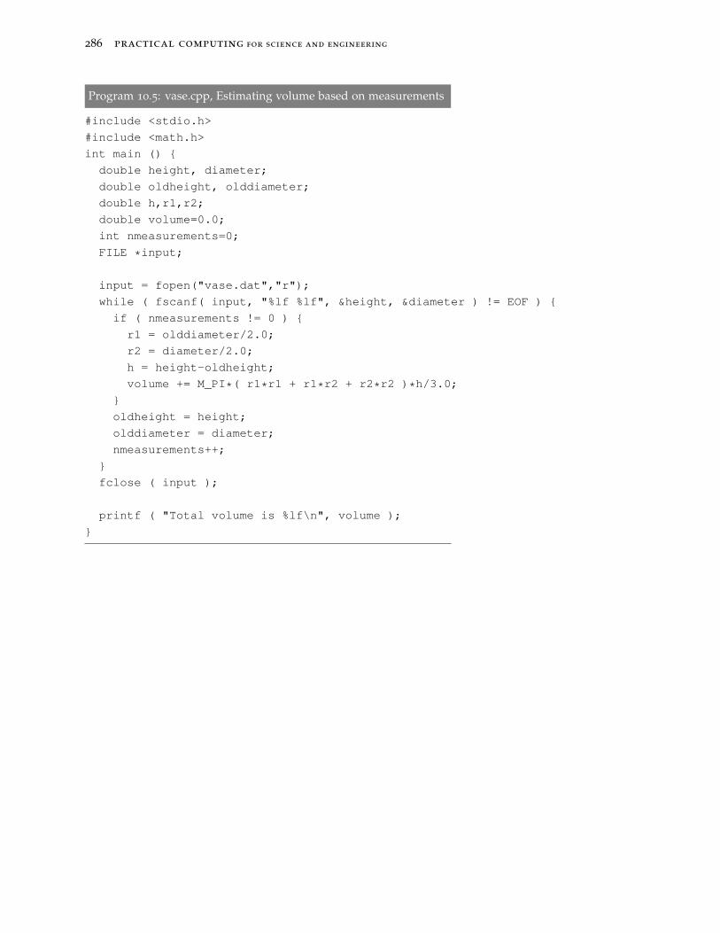
a file named vase.dat we could write a program like Program 10.5

(vase.cpp) to read the file and estimate the vase’s volume.

Notice that this program looks a look like our earlier roadtrip.cpp

program (Program 10.3). It uses the same strategy for reading an

unknown number of data points from a file and using the intervals

between them. The main difference is that now we’re calculating the

volumes of truncated cones, using the formula above, whereas in the

earlier program we were calculating the areas of trapezoids.

We could use this this new program to estimate the volume of any

cylindrically-symmetric shape, based on some measurements of height

and diameter stored in a data file.


Program 10.5: vase.cpp, Estimating volume based on measurements

#include <stdio.h>

#include <math.h>

int main () {

double height, diameter;

double oldheight, olddiameter;

double h,r1,r2;

double volume=0.0;

int nmeasurements=0;

FILE *input;

input = fopen("vase.dat","r");

while ( fscanf( input, "%lf %lf", &height, &diameter ) != EOF ) {

if ( nmeasurements != 0 ) {

r1 = olddiameter/2.0;

r2 = diameter/2.0;

h = height-oldheight;

volume += M_PI*( r1*r1 + r1*r2 + r2*r2 )*h/3.0;

}

oldheight = height;

olddiameter = diameter;

nmeasurements++;

}

fclose ( input );

printf ( "Total volume is %lf\n", volume );

}


Sometimes the volume we need to estimate won’t belong to a physical

object like a vase that we can take measurements from. We might be

given a mathematical function that describes a shape in 3-dimensional

space, and asked to find the volume inside it. This would be analogous

to the 2-dimensional integration of a function that we did earlier, in

Program 10.4.

Program 10.6 (vase-func.cpp) uses a function to describe the shape

of the vase’s side, then divides the vase’s height up into five truncated-

cone-shaped slices and adds up their volumes. It works just like

Program 10.4, but calculates the volumes of truncated-cone-shaped

slices instead of the areas of trapezoids. The function func at the top

defines the shape of the vase’s side, and the values xmin and xmax are

the bottom and top of the vase, respectively.

Again, this program could be used to estimate the volume of any

cylindrically-symmetric shape. We’d just need to change the definition

of func and xmin and xmax appropriately.

Program 10.6: vase-func.cpp, Estimating volume based on a function

#include <stdio.h>

#include <math.h>

double func( double x ) {

double value;

value = 1.5 + sin(x);

return(value);

}

int main () {

double x, volume=0;

double xmin=0.1, xmax=2.0*M_PI;

double r1, r2, h;

int i, nsteps=5;

h = (xmax-xmin)/nsteps;

x = xmin;


r1 = func(x);

r2 = func(x+h);

volume += M_PI*( r1*r1 + r1*r2 + r2*r2 )*h/3.0;

x += h;

}

printf ( "Integral from %lf to %lf is %lf\n",

xmin, xmax, volume );

}


10.11. Monte Carlo Integration

Figure 10.33: Chickens, finding the ap-proximate value of an integral.Source: Wikimedia Commons

Did you know that chickens can do calculus? It’s true. Let’s say we

wanted to find the area of the shaded shape in Figure 10.34. This could

be any shape, possibly one whose area can’t be exactly determined

mathematically. But, we’re smart chicken-farming programmers, so we

know how to find an approximate value for the area.

Figure 10.34: The ratio of pecks insidethe shape to pecks outside the shape isapproximately equal to the ratio of theshape’s area to the area of its enclosure.

We walk into our chickenyard and draw the shape on the ground, then

go away and let the chickens walk about, pecking at the ground. We

watch from a distance and count how many times they peck anywhere

in the yard, and keep a separate count of the number of times they peck

inside the shape we’ve drawn.

Now we’re all set to estimate the area of the weird shape we’ve drawn.

We know the dimensions of our chickenyard, and can calculate its area.

We know the total number of pecks in the chickenyard, and we know

how many of those pecks were inside the weird shape. To keep things

clear, let’s define some variables to represent these things:

Atotal = The total area of the chickenyard

ntotal = The total number of pecks

nshape = The number of pecks inside the shape

Ashape = The unknown area of the shape

If the total number of pecks is large and evenly spread through the

chickenyard we’d expect that the following will be true:

Ashape

Atotal=

nshape

ntotal

https://commons.wikimedia.org/wiki/File:Kluck_Kluck_(Boston_Public_Library).jpg


Or, rearranging a little, we could say that

Ashape = Atotal

nshape

ntotal(10.1)

We know all of the things on the right-hand side of this equation, so

we just need to plug them into a calculator to find Ashape.

Thanks Chickens!

Figure 10.35: "A balmy, restful peaceful-ness seemed to reign everywhere. Even theold hen seemed well satisfied. She scratchedamong the stones and called to her chickenswhen she found a treasure; and all thewhile clucked to herself with intense inwardsatisfaction. Waldo, as he sat with his kneesdrawn up to his chin and his arms foldedon them, looked at it all and smiled. An evilworld, a deceitful, treacherous, mirage-likeworld, it might be; but a lovely world forall that, and to sit there, gloating in thesunlight, was perfect. It was worth havingbeen a little child, and having cried andprayed, so one might sit there."—The Story of an African Farm, OliveSchreiner (1883).Source: Wikimedia Commons

Fortunately for those who live in apartments, we don’t need chickens in

order to use this technique. We can do the same thing with a computer

program.

As we’ve seen before, we can use the rand function to generate random

numbers. Instead of letting chickens peck, we can write a program that

generates pecks at random locations. Beyond that, the only thing our

program will need will be some way of knowing whether a particular

point lies inside the shape we’re interested in.

Let’s try doing it with a shape whose area we know exactly, so we can

see if our pecking technique really does do a good job of estimating the

area. Figure 10.36 shows a circular area inside a square chickenyard.

The circle has a radius of 1, and we know that the area of a circle is πr2,

so the area of this circle should be exactly π.

-1

-0.5

0

0.5

1

-1 -0.5 0 0.5 1

Figure 10.36: A circular area with a ra-dius of 1, inside a square 1 × 1 “chicken-yard”.

https://commons.wikimedia.org/wiki/File:Olive_Schreiner02.jpg


Program 10.7 estimates the area of the circle by simulating chicken

pecks. It generates 1,000 random peck positions inside the chicken

yard, then checks each peck to see if it’s inside our area of interest. The

program keeps track of the number of pecks inside the area. After it’s

done pecking, the program calculates the area by using Equation 10.1,

above.

Figure 10.37: A 3-d version of ourpecking scheme.

Note that each random peck position is created by generating random

values for x and y. We do this by multiplying the width or height of the

chickenyard by a random number between 0 and 1, and then adding

the result to the minimum x or y value.

The function inside tells the program whether a given peck lies inside

the area we’re interested in. it checks to see if√

x2 + y2 is less than or

equal to the circle’s radius. If the peck is inside, the function returns

the value “1”. Otherwise, it returns a “0”.

The inside function is the only part of the program that’s specific to

a circle. If we wanted to find the area of a different shape, we’d only

need to rewrite this function.

The program could be extended to three dimensions by adding a z

coordinate, and used to estimate volumes. In that case, we’d generate

random x, y, and z coordinate for each “peck”, and keep track of how

many landed inside a 3-d shape we were interested in (see Figure 10.37).

Figure 10.38: The Monte Carlo Casino,in the Principality of MonacoSource: Wikimedia Commons

The technique described in this section is known as “Monte Carlo

integration”. It takes its name from the gambling resort of Monte Carlo,

on the French Riviera. Like the dice-rolling gamblers at Monte Carlo,

our pecking program does its job by generating random numbers.

Figure 10.39: Consider the case of an11-dimensional integral in String The-ory. This might be utterly impossible tosolve exactly, but by generating thou-sands of sets of 11 coordinate values,we could estimate its value by MonteCarlo methods.Source: Wikimedia Commons

The Monte Carlo technique has several virtues:

• As we mentioned above, the Monte Carlo method can easily be

extended to higher dimensional problems.

• To use this technique you only need two things:

– You need a way to determine whether a point is inside the shape

you’re interested in, and

– You need to be able to draw a “chickenyard” of a known area that

completely encloses the shape.

• Although other methods are often more efficient for integrating 2-d

functions, the Monte Carlo technique is quite efficient for higher-

dimensional integrals.

https://commons.wikimedia.org/wiki/File:Le_casino_de_Monte-Carlo.JPG

https://commons.wikimedia.org/wiki/File:Calabi_yau.jpg


Program 10.7: peck.cpp

#include <stdio.h>

#include <stdlib.h>

#include <time.h>

#include <math.h>

int inside ( double x, double y ) {

double radius = 1.0;

if ( sqrt( x*x + y*y ) <= radius ) {

return ( 1 );

} else {

return ( 0 );

}

}

int main () {

double xmin = -1, xmax = 1;

double ymin = -1, ymax = 1;

double atotal;

double ashape;

double xrange, yrange, x, y;

int ntotal = 1000;

int peck;

int nshape=0;

xrange = xmax - xmin;

yrange = ymax - ymin;

srand(time(NULL));

for ( peck=0; peck<ntotal; peck++ ) {

x = xmin + xrange*rand()/(1.0+RAND_MAX);

y = ymin + yrange*rand()/(1.0+RAND_MAX);

if ( inside( x, y ) ) {

nshape++;

}

}

atotal = (xmax-xmin) * (ymax-ymin);

ashape = atotal * nshape/(double)ntotal;

printf ( "The area of the shape is %lf\n", ashape );

}


0

0.2

0.4

0.6

0.8

1

0 0.5 1 1.5 2 2.5 3

sin

(sin

(x))

x

Figure 10.40: Integrating sin(sin(x))using the Monte Carlo method.

Exercise 51: Chicken Pot Pi

Create, compile, and run Program 10.7. Does it give a good

approximation of the value of π? Try increasing the number

of pecks to 100,000. Does this improve the program’s results?

Now try integrating the sin(sin(x)) function again, this

time using the Monte Carlo technique. To do this, make a

modified version of Program 10.7 as follows:

• Copy peck.cpp to peck2.cpp:

cp peck.cpp peck2.cpp

• Change the inside function so it looks like this:

int inside ( double x, double y ) {

if ( y <= sin(sin(x)) ) {

return ( 1 );

} else {

return ( 0 );

}

}

• Change the limits of the “chickenyard” to these values:

double xmin = 0, xmax = M_PI;

double ymin = 0, ymax = 1;

Compile and run your new peck2.cpp program. Does

its result agree with the value you got earlier using the

trapezoid rule to integrate sin(sin(x))?

sin(x)dx = 2Figure 10.41: A chickintegral


10.12. Conclusion

Figure 10.42: As Mick Jagger says, “Youcan’t always get what you want, but ifyou try sometimes you just might findyou get what you need.”Source: Wikimedia Commons

The trapezoid rule and Monte Carlo integration techniques are both

useful tools for dealing with recalcitrant integrals. They let a program-

mer find approximate values for the area under a curve defined by data

points, and find arbitrarily precise approximations to a wide array of

definite integrals of functions, many of which can’t be solved exactly.

https://commons.wikimedia.org/wiki/File:Rolling_Stones_04.jpg


Practice Problems

-1

-0.5

0

0.5

1

0 0.5 1 1.5 2 2.5 3

x=π/2

Figure 10.43: A graph of the cosinefunction. The region between x = 0 andx = π/2 is shaded.

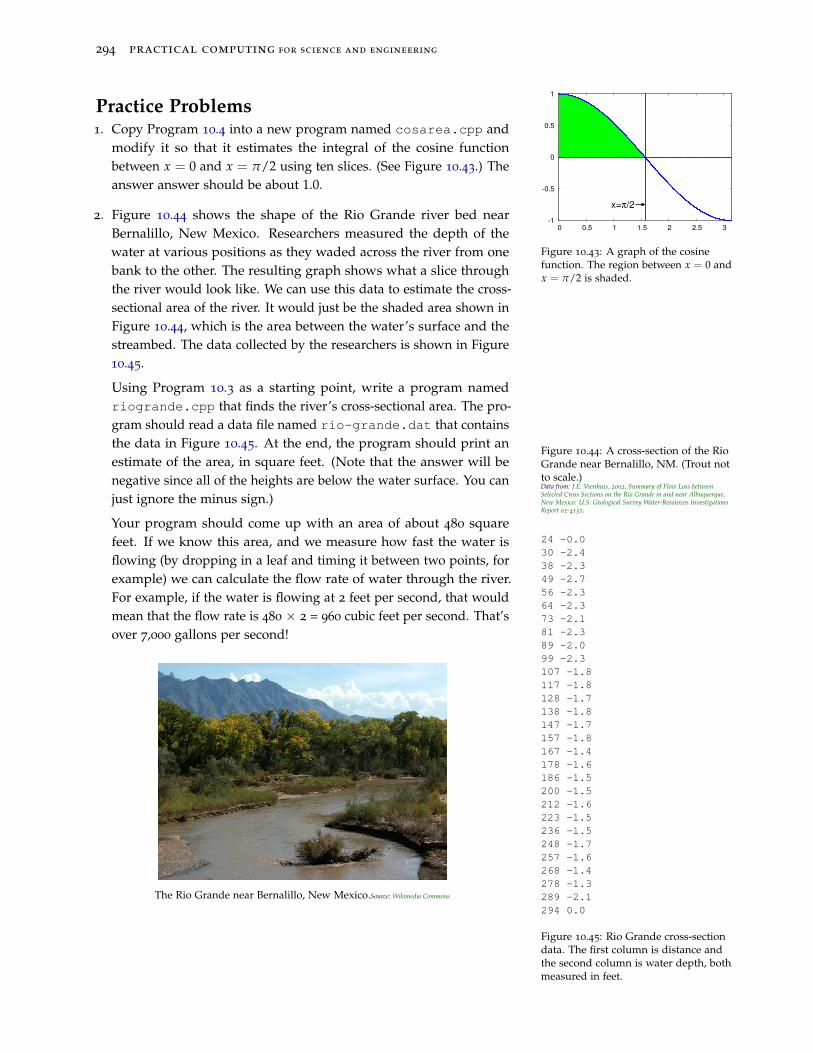
1. Copy Program 10.4 into a new program named cosarea.cpp and

modify it so that it estimates the integral of the cosine function

between x = 0 and x = π/2 using ten slices. (See Figure 10.43.) The

answer answer should be about 1.0.

Figure 10.44: A cross-section of the RioGrande near Bernalillo, NM. (Trout notto scale.)Data from: J.E. Veenhuis, 2002, Summary of Flow Loss betweenSelected Cross Sections on the Rio Grande in and near Albuquerque,New Mexico: U.S. Geological Survey Water-Resources InvestigationsReport 02-4131.

2. Figure 10.44 shows the shape of the Rio Grande river bed near

Bernalillo, New Mexico. Researchers measured the depth of the

water at various positions as they waded across the river from one

bank to the other. The resulting graph shows what a slice through

the river would look like. We can use this data to estimate the cross-

sectional area of the river. It would just be the shaded area shown in

Figure 10.44, which is the area between the water’s surface and the

streambed. The data collected by the researchers is shown in Figure

10.45.

24 -0.0

30 -2.4

38 -2.3

49 -2.7

56 -2.3

64 -2.3

73 -2.1

81 -2.3

89 -2.0

99 -2.3

107 -1.8

117 -1.8

128 -1.7

138 -1.8

147 -1.7

157 -1.8

167 -1.4

178 -1.6

186 -1.5

200 -1.5

212 -1.6

223 -1.5

236 -1.5

248 -1.7

257 -1.6

268 -1.4

278 -1.3

289 -2.1

294 0.0

Figure 10.45: Rio Grande cross-sectiondata. The first column is distance andthe second column is water depth, bothmeasured in feet.

Using Program 10.3 as a starting point, write a program named

riogrande.cpp that finds the river’s cross-sectional area. The pro-

gram should read a data file named rio-grande.dat that contains

the data in Figure 10.45. At the end, the program should print an

estimate of the area, in square feet. (Note that the answer will be

negative since all of the heights are below the water surface. You can

just ignore the minus sign.)

Your program should come up with an area of about 480 square

feet. If we know this area, and we measure how fast the water is

flowing (by dropping in a leaf and timing it between two points, for

example) we can calculate the flow rate of water through the river.

For example, if the water is flowing at 2 feet per second, that would

mean that the flow rate is 480 × 2 = 960 cubic feet per second. That’s

over 7,000 gallons per second!

The Rio Grande near Bernalillo, New Mexico.Source: Wikimedia Commons

https://pubs.usgs.gov/wri/wri02-4131/




https://en.wikipedia.org/wiki/File:BosqueNM.jpg


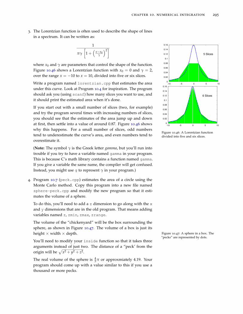
3. The Lorentzian function is often used to describe the shape of lines

in a spectrum. It can be written as:

1

πγ

[

1 +(

x−x0γ

)2]

where x0 and γ are parameters that control the shape of the function.

Figure 10.46 shows a Lorentzian function with x0 = 0 and γ = 2,

over the range x = −10 to x = 10, divided into five or six slices.

0

0.02

0.04

0.06

0.08

0.1

0.12

0.14

0.16

-10 -5 0 5 10

5 Slices

0

0.02

0.04

0.06

0.08

0.1

0.12

0.14

0.16

-10 -5 0 5 10

6 Slices

Figure 10.46: A Lorentzian functiondivided into five and six slices.

Write a program named lorentzian.cpp that estimates the area

under this curve. Look at Program 10.4 for inspiration. The program

should ask you (using scanf) how many slices you want to use, and

it should print the estimated area when it’s done.

If you start out with a small number of slices (two, for example)

and try the program several times with increasing numbers of slices,

you should see that the estimates of the area jump up and down

at first, then settle into a value of around 0.87. Figure 10.46 shows

why this happens. For a small number of slices, odd numbers

tend to underestimate the curve’s area, and even numbers tend to

overestimate it.

(Note: The symbol γ is the Greek letter gamma, but you’ll run into

trouble if you try to have a variable named gamma in your program.

This is because C’s math library contains a function named gamma.

If you give a variable the same name, the compiler will get confused.

Instead, you might use g to represent γ in your program.)

Figure 10.47: A sphere in a box. The“pecks” are represented by dots.

4. Program 10.7 (peck.cpp) estimates the area of a circle using the

Monte Carlo method. Copy this program into a new file named

sphere-peck.cpp and modify the new program so that it esti-

mates the volume of a sphere.

To do this, you’ll need to add a z dimension to go along with the x

and y dimensions that are in the old program. That means adding

variables named z, zmin, zmax, zrange.

The volume of the “chickenyard” will be the box surrounding the

sphere, as shown in Figure 10.47. The volume of a box is just its

height × width × depth.

You’ll need to modify your inside function so that it takes three

arguments instead of just two. The distance of a “peck’ from the

origin will be√

x2 + y2 + z2.

The real volume of the sphere is 43 π or approxmiately 4.19. Your

program should come up with a value similar to this if you use a

thousand or more pecks.


5. Find the approximate area under the curve y = 1 − x2 between

x = −1 and x = 1 (see Figure 10.48) using two different techniques:

0

0.2

0.4

0.6

0.8

1

-1 -0.5 0 0.5 1

1-x

*x

x

Figure 10.48: A parabolic area betweenx = −1 and x = 1.

(a) Copy Program 10.4 into a new file named parabola.cpp. Mod-

ify the new program so that, instead of finding the integral of the

sine function, it finds the integral of 1 − x2 over the range from

x = −1 to x = 1.

To do this, you’ll need to change the func function and you’ll

need to change the values of xmin and xmax.

Compile and run your program. It should find that the area is

approximately 43 . If the result you get initially isn’t very close, try

increasing the value of nsteps (the number of slices).

(b) Copy Program 10.7 into a new file named parabola-peck.cpp.

Modify the program so that it finds the integral of 1 − x2 over the

range from x = −1 to x = 1.

To do this, you’ll need to modify the inside function. The

function should return a 1 for points in the shaded region of Figure

10.48 and zero otherwise. (Hint: Check to see if y < 1-x*x.)

You’ll also need to change the bounds of your chickenyard, since

ymin should now be zero.


approximately 43 . If the result you get initially isn’t very close, try

increasing the value of ntotal (the number of pecks).


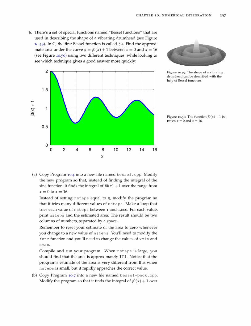
6. There’s a set of special functions named “Bessel functions” that are

used in describing the shape of a vibrating drumhead (see Figure

10.49). In C, the first Bessel function is called j0. Find the approxi-

mate area under the curve y = j0(x) + 1 between x = 0 and x = 16

(see Figure 10.50) using two different techniques, while looking to

see which technique gives a good answer more quickly:

Figure 10.49: The shape of a vibratingdrumhead can be described with thehelp of Bessel functions.

0

0.5

1

1.5

2

0 2 4 6 8 10 12 14 16

j0(x

) +

1

x

Figure 10.50: The function j0(x) + 1 be-tween x = 0 and x = 16.

(a) Copy Program 10.4 into a new file named bessel.cpp. Modify

the new program so that, instead of finding the integral of the

sine function, it finds the integral of j0(x) + 1 over the range from

x = 0 to x = 16.

Instead of setting nsteps equal to 5, modify the program so

that it tries many different values of nsteps. Make a loop that

tries each value of nsteps between 1 and 1,000. For each value,

print nsteps and the estimated area. The result should be two

columns of numbers, separated by a space.

Remember to reset your estimate of the area to zero whenever

you change to a new value of nsteps. You’ll need to modify the

func function and you’ll need to change the values of xmin and

xmax.

Compile and run your program. When nsteps is large, you

should find that the area is approximately 17.1. Notice that the

program’s estimate of the area is very different from this when

nsteps is small, but it rapidly appraches the correct value.

(b) Copy Program 10.7 into a new file named bessel-peck.cpp.

Modify the program so that it finds the integral of j0(x) + 1 over


the range from x = 0 to x = 16.

Instead of setting ntotal to 1,000, try different values of ntotal.

Make a loop that tries each value of ntotal between 1 and 1,000.

For each value, print ntotal and the estimated area. The result

should be two columns of numbers, separated by a space.

Remember to reset nshape to zero whenever you change the

value of ntotal. You’ll need to modify the inside function. The

function should return a 1 for points in the shaded region of Figure

10.50 and zero otherwise. (Hint: Check to see if y<j0(x)-1.)

You’ll also need to change the bounds of your chickenyard, since

xmin and ymin should now be zero, and xmax should be 16.


approximately 17.1. Notice that the program eventually gets close

to this value, but not until ntotal is pretty large.

If we ran our two programs like this:

./bessel > bessel.dat

./bessel-peck > bessel-peck.dat

we could compare the two output files by plotting them with gnu-

plot. The result is shown in Figure 10.51. The vertical axis shows

our estimate of the area and the horizontal axis shows how many

slices or pecks we needed to get that estimate. As you can see, the

Monte Carlo program bessel-peck.cpp eventually gets close to

the right answer, but it takes many “pecks” to get there. The other

program (bessel.cpp) gets close to the right answer after only a

few trapezoidal slices, and stays there from then on.

0

5

10

15

20

25

1 10 100 1000

Appro

xim

ate

Are

a

Number of Slices or Pecks

Monte CarloTrapezoid

Figure 10.51: A comparison of area esti-mates for different values of nsteps orntotal. Notice that the x axis is loga-rithmic, so we can pack a large range intoit while still being able to see the smallvalues. In gnuplot you can do this by say-ing set log x before you use the plotcommand.


-1

-0.5

0

0.5

1

-1.5 -1 -0.5 0 0.5 1 1.5

y

x

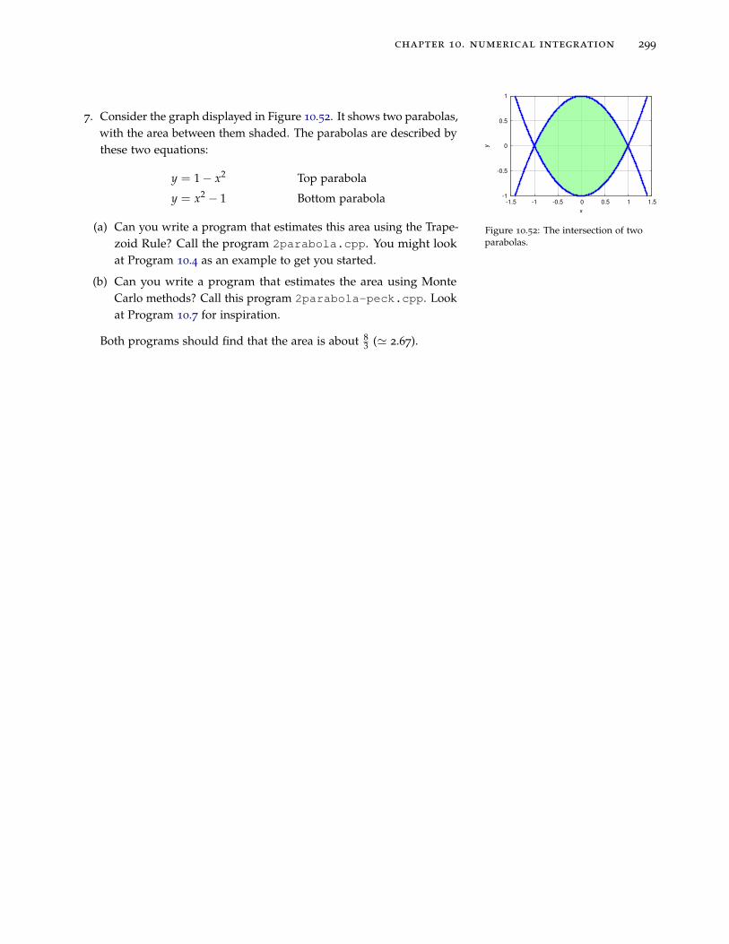
Figure 10.52: The intersection of twoparabolas.

7. Consider the graph displayed in Figure 10.52. It shows two parabolas,

with the area between them shaded. The parabolas are described by

these two equations:

y = 1 − x2 Top parabola

y = x2− 1 Bottom parabola

(a) Can you write a program that estimates this area using the Trape-

zoid Rule? Call the program 2parabola.cpp. You might look

at Program 10.4 as an example to get you started.

(b) Can you write a program that estimates the area using Monte

Carlo methods? Call this program 2parabola-peck.cpp. Look

at Program 10.7 for inspiration.

Both programs should find that the area is about 83 (≃ 2.67).

10. Numerical Integration - Galileogalileo.phys.virginia.edu/compfac/courses/practical-c/10.pdf ·...

Documents

Transcript of 10. Numerical Integration - Galileogalileo.phys.virginia.edu/compfac/courses/practical-c/10.pdf ·...