10 Mitigation Potential and Costs

791

10 Mitigation Potentialand Costs

Coordinating Lead Authors:Manfred Fischedick (Germany) and Roberto Schaeffer (Brazil)

Lead Authors: Akintayo Adedoyin (Botswana), Makoto Akai (Japan), Thomas Bruckner (Germany), Leon Clarke (USA), Volker Krey (Austria/Germany), Ilkka Savolainen (Finland), Sven Teske (Germany), Diana Ürge-Vorsatz (Hungary), Raymond Wright † (Jamaica)

Contributing Authors:Gunnar Luderer (Germany)

Review Editors: Erin Baker (USA) and Keywan Riahi (Austria)

This chapter should be cited as:

Fischedick, M., R. Schaeffer, A. Adedoyin, M. Akai, T. Bruckner, L. Clarke, V. Krey, I. Savolainen, S. Teske,

D. Ürge-Vorsatz, R. Wright, 2011: Mitigation Potential and Costs. In IPCC Special Report on Renewable Energy

Sources and Climate Change Mitigation [O. Edenhofer, R. Pichs-Madruga, Y. Sokona, K. Seyboth, P. Matschoss,

S. Kadner, T. Zwickel, P. Eickemeier, G. Hansen, S. Schlömer, C. von Stechow (eds)], Cambridge University Press,

Cambridge, United Kingdom and New York, NY, USA.

792

Mitigation Potential and Costs Chapter 10

Table of Contents

Executive Summary . . . . . . . . . . . . . . . . . . . . . . . . . . . . . . . . . . . . . . . . . . . . . . . . . . . . . . . . . . . . . . . . . . . . . . . . . . . . . . . . . . . . . . . . . . . . . . . . . . . . . . . . . . . . . . . . . . . . . . . . . . . . . . . . . . . . . . . . . . . . . 794

10.1 Introduction . . . . . . . . . . . . . . . . . . . . . . . . . . . . . . . . . . . . . . . . . . . . . . . . . . . . . . . . . . . . . . . . . . . . . . . . . . . . . . . . . . . . . . . . . . . . . . . . . . . . . . . . . . . . . . . . . . . . . . . . . . . . . . . . . . . . . . . . . 798

10.2 Synthesis of mitigation scenarios for different renewable energy strategies . . . . . . . . . . . . . . . . . . . . . . . . . . . 799

10.2.1 State of scenario analysis . . . . . . . . . . . . . . . . . . . . . . . . . . . . . . . . . . . . . . . . . . . . . . . . . . . . . . . . . . . . . . . . . . . . . . . . . . . . . . . . . . . . . . . . . . . . . . . . . . . . . . . . . . . . . . . . . . . . . . . . . . . 79910.2.1.1 Types of scenario methods . . . . . . . . . . . . . . . . . . . . . . . . . . . . . . . . . . . . . . . . . . . . . . . . . . . . . . . . . . . . . . . . . . . . . . . . . . . . . . . . . . . . . . . . . . . . . . . . . . . . . . . . . . . . . . . . . . . . . . . . . . . . . 79910.2.1.2 Strengths and weaknesses of quantitative scenarios . . . . . . . . . . . . . . . . . . . . . . . . . . . . . . . . . . . . . . . . . . . . . . . . . . . . . . . . . . . . . . . . . . . . . . . . . . . . . . . . . . . . . . . . . . . . . . 800

10.2.2 The role of renewable energy sources in scenarios . . . . . . . . . . . . . . . . . . . . . . . . . . . . . . . . . . . . . . . . . . . . . . . . . . . . . . . . . . . . . . . . . . . . . . . . . . . . . . . . . . . . . . . . . 80010.2.2.1 Overview of the scenarios reviewed in this section . . . . . . . . . . . . . . . . . . . . . . . . . . . . . . . . . . . . . . . . . . . . . . . . . . . . . . . . . . . . . . . . . . . . . . . . . . . . . . . . . . . . . . . . . . . . . . . . 80010.2.2.2 Overview of the role of renewable energy in the scenarios . . . . . . . . . . . . . . . . . . . . . . . . . . . . . . . . . . . . . . . . . . . . . . . . . . . . . . . . . . . . . . . . . . . . . . . . . . . . . . . . . . . . . . 80110.2.2.3 Setting the scale of renewable energy deployment: Energy system growth and long-term climate goals . . . . . . . . . . . . . . . . . . . . . . . . . . . . . . 80310.2.2.4 Competition between renewable energy sources and other forms of low-carbon energy . . . . . . . . . . . . . . . . . . . . . . . . . . . . . . . . . . . . . . . . . . . . . . . . . . 80510.2.2.5 Renewable energy deployment by technology, over time and by region . . . . . . . . . . . . . . . . . . . . . . . . . . . . . . . . . . . . . . . . . . . . . . . . . . . . . . . . . . . . . . . . . . . . . . 80610.2.2.6 Renewable energy and the costs of mitigation . . . . . . . . . . . . . . . . . . . . . . . . . . . . . . . . . . . . . . . . . . . . . . . . . . . . . . . . . . . . . . . . . . . . . . . . . . . . . . . . . . . . . . . . . . . . . . . . . . . . . 808

10.2.3 The deployment of renewable energy sources in scenarios from the technology perspective . . . . . . . . . . . . . . . . . . . . . . . . . . . . . . . . 812

10.2.4 Knowledge gaps . . . . . . . . . . . . . . . . . . . . . . . . . . . . . . . . . . . . . . . . . . . . . . . . . . . . . . . . . . . . . . . . . . . . . . . . . . . . . . . . . . . . . . . . . . . . . . . . . . . . . . . . . . . . . . . . . . . . . . . . . . . . . . . . . . . . . . . 812

10.3 Assessment of representative mitigation scenarios for different renewable energy strategies . . . . . . . . . . . . . . . . . . . . . . . . . . . . . . . . . . . . . . . . . . . . . . . . . . . . . . . . . . . . . . . . . . . . . . . . . . . . . . . . . . . . . . . . . . . . . . . . . . . . . . . . . . . . . . . . . . . . . . . . . . . . . . . . . . . . . . . . . . . . . 813

10.3.1 Sectoral breakdown of renewable energy sources . . . . . . . . . . . . . . . . . . . . . . . . . . . . . . . . . . . . . . . . . . . . . . . . . . . . . . . . . . . . . . . . . . . . . . . . . . . . . . . . . . . . . . . . . . 81310.3.1.1 Renewable energy deployment in the electricity sector . . . . . . . . . . . . . . . . . . . . . . . . . . . . . . . . . . . . . . . . . . . . . . . . . . . . . . . . . . . . . . . . . . . . . . . . . . . . . . . . . . . . . . . . . . . 81610.3.1.2 Renewable energy deployment in the heating and cooling sector . . . . . . . . . . . . . . . . . . . . . . . . . . . . . . . . . . . . . . . . . . . . . . . . . . . . . . . . . . . . . . . . . . . . . . . . . . . . . . 81810.3.1.3 Renewable energy deployment in the transport sector . . . . . . . . . . . . . . . . . . . . . . . . . . . . . . . . . . . . . . . . . . . . . . . . . . . . . . . . . . . . . . . . . . . . . . . . . . . . . . . . . . . . . . . . . . . 82010.3.1.4 Global renewable energy primary energy contribution . . . . . . . . . . . . . . . . . . . . . . . . . . . . . . . . . . . . . . . . . . . . . . . . . . . . . . . . . . . . . . . . . . . . . . . . . . . . . . . . . . . . . . . . . . . . 820

10.3.2 Regional breakdown – technical potential versus market deployment . . . . . . . . . . . . . . . . . . . . . . . . . . . . . . . . . . . . . . . . . . . . . . . . . . . . . . . . . . . . . . . 82010.3.2.1 Regional renewable energy supply curves . . . . . . . . . . . . . . . . . . . . . . . . . . . . . . . . . . . . . . . . . . . . . . . . . . . . . . . . . . . . . . . . . . . . . . . . . . . . . . . . . . . . . . . . . . . . . . . . . . . . . . . . . . . 82010.3.2.2 Primary energy by region, technology and sector . . . . . . . . . . . . . . . . . . . . . . . . . . . . . . . . . . . . . . . . . . . . . . . . . . . . . . . . . . . . . . . . . . . . . . . . . . . . . . . . . . . . . . . . . . . . . . . . . . 825

10.3.3 Greenhouse gas mitigation potential of renewable energy in aggregate and as individual options . . . . . . . . . . . . . . . . . . . . . . . 826

10.3.4 Comparison of the results of the in-depth scenario analysis and knowledge gaps . . . . . . . . . . . . . . . . . . . . . . . . . . . . . . . . . . . . . . . . . . . . . . . 830

10.4 Regional cost curves for mitigation with renewable energies . . . . . . . . . . . . . . . . . . . . . . . . . . . . . . . . . . . . . . . . . . . . . . . . . . . . . 832

10.4.1 Introduction . . . . . . . . . . . . . . . . . . . . . . . . . . . . . . . . . . . . . . . . . . . . . . . . . . . . . . . . . . . . . . . . . . . . . . . . . . . . . . . . . . . . . . . . . . . . . . . . . . . . . . . . . . . . . . . . . . . . . . . . . . . . . . . . . . . . . . . . . . . . . 832

793

Chapter 10 Mitigation Potential and Costs

10.4.2 Cost curves: concept, strengths and limitations . . . . . . . . . . . . . . . . . . . . . . . . . . . . . . . . . . . . . . . . . . . . . . . . . . . . . . . . . . . . . . . . . . . . . . . . . . . . . . . . . . . . . . . . . . . . . . 83210.4.2.1 The concept . . . . . . . . . . . . . . . . . . . . . . . . . . . . . . . . . . . . . . . . . . . . . . . . . . . . . . . . . . . . . . . . . . . . . . . . . . . . . . . . . . . . . . . . . . . . . . . . . . . . . . . . . . . . . . . . . . . . . . . . . . . . . . . . . . . . . . . . . . . . . . . 83210.4.2.2 Limitations of the supply curve method . . . . . . . . . . . . . . . . . . . . . . . . . . . . . . . . . . . . . . . . . . . . . . . . . . . . . . . . . . . . . . . . . . . . . . . . . . . . . . . . . . . . . . . . . . . . . . . . . . . . . . . . . . . . . . 833

10.4.3 Review of regional energy and abatement cost curves from the literature . . . . . . . . . . . . . . . . . . . . . . . . . . . . . . . . . . . . . . . . . . . . . . . . . . . . . . . . . 83410.4.3.1 Introduction . . . . . . . . . . . . . . . . . . . . . . . . . . . . . . . . . . . . . . . . . . . . . . . . . . . . . . . . . . . . . . . . . . . . . . . . . . . . . . . . . . . . . . . . . . . . . . . . . . . . . . . . . . . . . . . . . . . . . . . . . . . . . . . . . . . . . . . . . . . . . . . 83410.4.3.2 Regional and global renewable energy supply curves . . . . . . . . . . . . . . . . . . . . . . . . . . . . . . . . . . . . . . . . . . . . . . . . . . . . . . . . . . . . . . . . . . . . . . . . . . . . . . . . . . . . . . . . . . . . . 83410.4.3.3 Regional and global carbon abatement cost curves . . . . . . . . . . . . . . . . . . . . . . . . . . . . . . . . . . . . . . . . . . . . . . . . . . . . . . . . . . . . . . . . . . . . . . . . . . . . . . . . . . . . . . . . . . . . . . . 834

10.4.4 Review of selected technology resource cost curves . . . . . . . . . . . . . . . . . . . . . . . . . . . . . . . . . . . . . . . . . . . . . . . . . . . . . . . . . . . . . . . . . . . . . . . . . . . . . . . . . . . . . . . 836

10.4.5 Gaps in knowledge . . . . . . . . . . . . . . . . . . . . . . . . . . . . . . . . . . . . . . . . . . . . . . . . . . . . . . . . . . . . . . . . . . . . . . . . . . . . . . . . . . . . . . . . . . . . . . . . . . . . . . . . . . . . . . . . . . . . . . . . . . . . . . . . . . . . 840

10.5 Costs of commercialization and deployment . . . . . . . . . . . . . . . . . . . . . . . . . . . . . . . . . . . . . . . . . . . . . . . . . . . . . . . . . . . . . . . . . . . . . . . . . . . . . . . . . . 841

10.5.1 Introduction: Review of present technology costs . . . . . . . . . . . . . . . . . . . . . . . . . . . . . . . . . . . . . . . . . . . . . . . . . . . . . . . . . . . . . . . . . . . . . . . . . . . . . . . . . . . . . . . . . . . 841

10.5.2 Prospects for cost decreases . . . . . . . . . . . . . . . . . . . . . . . . . . . . . . . . . . . . . . . . . . . . . . . . . . . . . . . . . . . . . . . . . . . . . . . . . . . . . . . . . . . . . . . . . . . . . . . . . . . . . . . . . . . . . . . . . . . . . . . 846

10.5.3 Deployment cost curves and learning investments . . . . . . . . . . . . . . . . . . . . . . . . . . . . . . . . . . . . . . . . . . . . . . . . . . . . . . . . . . . . . . . . . . . . . . . . . . . . . . . . . . . . . . . . . 849

10.5.4 Time-dependent expenditures . . . . . . . . . . . . . . . . . . . . . . . . . . . . . . . . . . . . . . . . . . . . . . . . . . . . . . . . . . . . . . . . . . . . . . . . . . . . . . . . . . . . . . . . . . . . . . . . . . . . . . . . . . . . . . . . . . . . . 849

10.5.5 Market support and research, development, demonstration and deployment . . . . . . . . . . . . . . . . . . . . . . . . . . . . . . . . . . . . . . . . . . . . . . . . . . . . . 851

10.5.6 Knowledge gaps . . . . . . . . . . . . . . . . . . . . . . . . . . . . . . . . . . . . . . . . . . . . . . . . . . . . . . . . . . . . . . . . . . . . . . . . . . . . . . . . . . . . . . . . . . . . . . . . . . . . . . . . . . . . . . . . . . . . . . . . . . . . . . . . . . . . . . . 851

10.6 Social and environmental costs and benefi ts . . . . . . . . . . . . . . . . . . . . . . . . . . . . . . . . . . . . . . . . . . . . . . . . . . . . . . . . . . . . . . . . . . . . . . . . . . . . . . . . 851

10.6.1 Background and objective . . . . . . . . . . . . . . . . . . . . . . . . . . . . . . . . . . . . . . . . . . . . . . . . . . . . . . . . . . . . . . . . . . . . . . . . . . . . . . . . . . . . . . . . . . . . . . . . . . . . . . . . . . . . . . . . . . . . . . . . . 851

10.6.2 Review of studies on external costs and benefi ts . . . . . . . . . . . . . . . . . . . . . . . . . . . . . . . . . . . . . . . . . . . . . . . . . . . . . . . . . . . . . . . . . . . . . . . . . . . . . . . . . . . . . . . . . . . 85310.6.2.1 Climate change . . . . . . . . . . . . . . . . . . . . . . . . . . . . . . . . . . . . . . . . . . . . . . . . . . . . . . . . . . . . . . . . . . . . . . . . . . . . . . . . . . . . . . . . . . . . . . . . . . . . . . . . . . . . . . . . . . . . . . . . . . . . . . . . . . . . . . . . . . 85310.6.2.2 Health impacts due to air pollution . . . . . . . . . . . . . . . . . . . . . . . . . . . . . . . . . . . . . . . . . . . . . . . . . . . . . . . . . . . . . . . . . . . . . . . . . . . . . . . . . . . . . . . . . . . . . . . . . . . . . . . . . . . . . . . . . . . 85410.6.2.3 Other impacts . . . . . . . . . . . . . . . . . . . . . . . . . . . . . . . . . . . . . . . . . . . . . . . . . . . . . . . . . . . . . . . . . . . . . . . . . . . . . . . . . . . . . . . . . . . . . . . . . . . . . . . . . . . . . . . . . . . . . . . . . . . . . . . . . . . . . . . . . . . . . 854

10.6.3 Social and environmental costs and benefi ts by energy sources and regional considerations . . . . . . . . . . . . . . . . . . . . . . . . . . . . . . . . 854

10.6.4 Synergistic strategies for limiting damages and external costs . . . . . . . . . . . . . . . . . . . . . . . . . . . . . . . . . . . . . . . . . . . . . . . . . . . . . . . . . . . . . . . . . . . . . . . . . 857

10.6.5 Knowledge gaps . . . . . . . . . . . . . . . . . . . . . . . . . . . . . . . . . . . . . . . . . . . . . . . . . . . . . . . . . . . . . . . . . . . . . . . . . . . . . . . . . . . . . . . . . . . . . . . . . . . . . . . . . . . . . . . . . . . . . . . . . . . . . . . . . . . . . . . 857

References . . . . . . . . . . . . . . . . . . . . . . . . . . . . . . . . . . . . . . . . . . . . . . . . . . . . . . . . . . . . . . . . . . . . . . . . . . . . . . . . . . . . . . . . . . . . . . . . . . . . . . . . . . . . . . . . . . . . . . . . . . . . . . . . . . . . . . . . . . . . . . . . . . . . . . . . . . . . 858

794


Executive Summary

Renewable energy (RE) has the potential to play an important and increasing role in achieving ambitious climate mitigation targets. Many RE technologies are increasingly becoming market competitive, although some innovative RE technologies are not yet mature, economic alternatives to non-RE technologies. However, assessing the future role of RE requires not only consideration of the cost and performance of RE technologies, but also an integrative perspective that takes into account the interactions between various forces and the overall systems behaviours.

An increasing number of integrated scenario analyses are available in the published literature. They are able to provide relevant insights into the potential contribution of RE to future energy supplies and climate change mitigation. A review of 164 scenarios from 16 different large-scale integrated models was conducted through an open call. Although a collection of scenarios from the literature does not represent a truly random sample suitable for rigorous statistical analysis, a scenario overview can provide some critical and strategic insights about the role of RE in climate mitigation, in spite of the uncertainties involved.

Although it is not possible to precisely link long-term climate goals and global RE deployment levels, RE deployment signifi cantly increases in the scenarios with ambitious greenhouse gas (GHG) concentration stabilization levels. Ambitious GHG concentration stabilization levels lead on average to higher RE deployment com-pared to the baseline. However, for any given long-term GHG concentration goal, the scenarios exhibit a wide range of RE deployment levels. In scenarios that stabilize the atmospheric carbon dioxide (CO2) concentration at a level of less than 440 ppm, the median RE deployment levels are 139 EJ/yr in 2030 and 248 EJ/yr in 2050, with the highest levels reaching 252 EJ/yr in 2030 and up to 428 EJ/yr in 2050. This range is a result of differences in assumptions about factors such as: developments in RE technologies and their associated resource bases and costs; comparative attrac-tiveness of competing mitigation options (i.e., end-use energy effi ciency, nuclear energy and fossil energy with carbon capture and storage (CCS)); fundamental drivers of energy services demand (including population, economic growth); the ability to integrate variable RE sources into power grids; fossil fuel resources; specifi c policy approaches to miti-gation; and emissions pathways towards long-term goals (e.g., overshoot versus stabilization). However, despite the observed variation, the scenarios indicate that, all else being equal, more ambitious mitigation generally leads to greater deployment of RE.

The majority of the 164 recent scenarios indicate a substantial increase in the deployment of RE by 2030, 2050 and beyond. In 2008, total RE production stood at roughly 64 EJ/yr (12.9% of total primary energy supply) with more than 30 EJ/yr of this being traditional biomass. More than 50% of the scenarios project levels of RE deployment in 2050 of more than 173 EJ/yr reaching up to over 400 EJ/yr in some cases. Given that traditional biomass demand decreases in most scenarios, an increase in the production level of RE (excluding traditional biomass) anywhere from roughly three-fold to more than ten-fold is projected. The global primary energy supply share of RE differs substantially among the scenarios. More than half of the scenarios show a contribution from RE in excess of a 17% share of primary energy supply in 2030, rising to more than 27% in 2050. The scenarios with the highest RE shares reach approximately 43% in 2030 and 77% in 2050. In other words, it is likely that RE will have a signifi cantly larger role (in absolute and relative numbers) in the global energy system in the future than today.

Even without efforts to address climate change RE can be expected to expand. Most baseline scenarios with no assumed climate mitigation policy show RE deployments signifi cantly above the 2008 level of 64 EJ/yr—up to 120 EJ/yr by 2030. By 2050 many baseline scenarios reach RE deployment levels of more than 100 EJ/yr, in some cases up to about 250 EJ/yr. These substantial deployment levels result from a range of assumptions, including, for example, the assumption that energy service demand will continue to grow substantially throughout the century and assumptions about the ability of RE to contribute to increased energy access and the limited long-term availability of fossil resources. Other assumptions (e.g., improved costs and performance of RE technologies) render RE technologies increasingly eco-nomically competitive in many applications even in the absence of climate policy.

795


RE deployment signifi cantly increases in scenarios with low GHG stabilization concentrations. Low GHG stabi-lization scenarios lead on average to higher RE deployment compared to the baseline. However, for any given long-term GHG concentration goal, the scenarios exhibit a wide range of RE deployment levels (Figure 10.2). In scenarios that stabilize atmospheric CO2 concentrations at a level of less than 440 ppm, the median RE deployment level in 2050 is 248 EJ/yr (139 EJ/yr in 2030), with the highest levels reaching 428 EJ/yr by 2050.

Many combinations of low-carbon energy supply options and energy effi ciency improvements can con-tribute to given low GHG concentration levels, with RE becoming the dominant low- carbon energy supply option by 2050 in the majority of scenarios. Ambitious GHG concentration stabilization levels lead, on average, to higher RE deployment compared to the baseline, with above 400 EJ/yr by 2050 as the upper limit of RE deployment. Many scenarios were constructed as sensitivities with explicit limits on the deployment of nuclear energy and CCS, and RE played an increasingly important role in these scenarios. Yet even in scenarios with no explicit limits on these com-peting low-carbon options, RE often represents well over 50% of the global primary energy supply.

Scenarios generally indicate that growth in RE will be widespread around the world. Although the precise distribution of RE deployment across regions substantially varies across scenarios, they are largely consistent in indicat-ing widespread growth in RE deployment around the globe. In addition, scenarios suggest that RE deployment levels will be higher over the long term in the group of non-Annex I countries than in the group of Annex I countries, in part a refl ection of the fact that non-Annex I countries are expected to represent an increasing share of total global energy demand over the coming decades.

Scenarios do not indicate an obvious single dominant RE technology at a global level. Besides the aspect that all RE obtains a more important role in the scenarios over time, a general trend is that bioenergy (predominantly modern biomass), wind energy and solar energy are commonly characterized by the largest contributions to the energy system among RE technologies by 2050.

Individual studies indicate that if RE deployment is limited, mitigation costs increase and low GHG stabili-zation concentrations may not be achieved. A number of studies have pursued scenario sensitivities that assume constraints on the deployment of individual mitigation options, including RE as well as nuclear and fossil energy with CCS. These studies indicate that mitigation costs are higher when options, including RE, are not available, but there is little agreement on the precise magnitude of the increase in costs. They also indicate that more ambitious GHG concen-tration goals may not be achievable when RE options are not available.

An in-depth analysis of four selected illustrative scenarios from the larger set of 164 scenarios allowed a more detailed look at the possible contribution of specifi c RE technologies in different regions and sectors. Even within this smaller set, the role of RE varies substantially, in part because the scenarios are aimed at different long-term climate goals, and because they are based on different assumptions about technology costs and also on dis-tinct scenario methodologies.

In the four representative scenarios, the RE-based electricity generation develops most quickly, at least in the medium term, followed by RE for heating/cooling and transport. For RE-based electricity generation, the highest market shares are expected in the analyzed time span. In contrast, currently the heating sector in many regions of the world is one of the most dominant demand sectors. Its RE share is high, especially in non-Annex I coun-tries, but it is mainly based on traditional bioenergy. The total share of RE-based electricity production for the four illustrative scenarios varies for the year 2050 (2030) from 24% (20%) up to 95% (61%) (cf. 19% RE-based electricity share in 2008). The corresponding range for the contribution of RE to the heating sector for these four scenarios lies for the year 2050 (2030) between 21% (20%) and 91% (49%). In most of the scenarios the heating and, particularly, the transport sector are less highlighted, showing that more importance should be given to thermal and transport RE applications in future studies.

796


Scenarios indicate that overall global technical potentials will not constrain the future contribution of RE. Although deployment of the different RE technologies signifi cantly increases over time, the resulting contribution of RE in the scenarios for most technologies is much lower than their corresponding technical potentials. In the four illus-trative scenarios, for instance, despite signifi cant technological and regional differences less than 2.5% of the global available technical RE potential is used. In this sense, scenario results confi rm that technical potentials will not be the limiting factors for the expansion of RE on a global scale.

Increasing sectoral shares of RE can substantially contribute to GHG mitigation. The four in-depth analyzed illustrative scenarios span a range of global cumulative CO2 savings, from about 220 to 560 Gt CO2 between 2010 and 2050 compared to about 1,530 Gt CO2 cumulative fossil and industrial CO2 emissions in the IEA World Energy Outlook 2009 Reference Scenario during the same period. The precise attribution of mitigation potentials to RE not only depends on the role scenarios attribute to specifi c mitigation technologies, but also on complex systems behaviours and, in particular, on the energy sources that RE displaces. Therefore, attribution of precise mitigation potentials to RE should be viewed with appropriate caution.

Scenarios often do not directly associate mitigation potentials with different technological options. Instead, abatement cost curves are often used to discuss and to compare different mitigation strategies. Abatement cost curves and energy supply curves are an approach that is very often used for discussing mitigation strategies and prioritizing abatement options. One of the most important strengths of this method is that the results can be understood easily and that the outcomes of these methods give, at fi rst glance, a clear orientation as they rank available options in order of cost-effectiveness. On the other hand, abatement cost curves have important limita-tions. In contrast to scenario analysis, they are not able to refl ect the complex system behaviour and corresponding interdependencies. Thus they have to rely on simplifi ed assumptions about the substituted non-RE supply and cor-responding emission factors. In general, it is very diffi cult to compare data and fi ndings from RE abatement cost and supply curves, as there have been very few studies using a comprehensive and consistent approach and detailing their methodologies, and most studies use different assumptions. Many of the regional and country studies provide less than 10% abatement of the baseline CO2 emissions over the medium term at abatement costs under around USD2005 100/t CO2. The resulting low-cost abatement potentials are quite low compared to the reported mitigation potentials of many of the scenarios reviewed here.

Some RE technologies are broadly competitive with current market energy prices. Many of the other RE technologies can provide competitive energy services in certain circumstances, for example, in regions with favourable resource conditions or that lack the infrastructure for other low-cost energy supplies. In most regions of the world, how-ever, policy measures are still required to ensure rapid deployment of many RE sources.

In the fi eld of RE, signifi cant opportunities exist to further improve the energy effi ciencies, and/or to decrease the costs of producing and installing the respective technologies. Together, these effects are expected to decrease the levelized cost of energy of many innovative RE-sourcing technologies in the future. Over time, energy generation costs of many RE technologies have shown signifi cant declines. In general, his-torical cost decreases can be described by experience curves with global learning rates (the relationship between the reduction in cost and a doubling of production).

To realize the learning effects and to allow an increase in the competitiveness of RE technologies, upfront investments in deployment, as well as research and development, will be needed, which will result in new market opportunities for RE suppliers. The four illustrative scenarios analyzed in detail in this Special Report esti-mate global cumulative RE investments (in the power generation sector only) ranging from USD2005 1,360 to 5,100 billion for the decade 2011 to 2020, and from USD2005 1,490 to 7,180 billion for the decade 2021 to 2030. The lower

797


values refer to the IEA World Energy Outlook 2009 Reference Scenario and the higher ones to a scenario that seeks to stabilize atmospheric CO2 (only) concentration at 450 ppm. The annual averages of these investment needs are all smaller than 1% of the world’s gross domestic product (GDP). The average annual investments in the reference scenario are slightly lower than the respective investments reported for 2009. Between 2011 and 2020, the higher end of the range of the annual averages of the RE electricity sector investments approximately correspond to a three-fold increase in the current global investments in this fi eld. For the next decade (2021 to 2030), a fi ve-fold increase is projected.

Increasing the installed capacity of RE power plants will reduce the amount of fossil and nuclear fuels that otherwise would be needed in order to meet a given electricity demand. In addition to investment, operation and maintenance (O&M) and (where applicable) feedstock costs related to RE power plants, any assessment of the overall economic burden that is associated with their application will therefore have to consider avoided fuel and substituted invest-ment costs as well.

Assessments of the costs of future paths of RE deployment and mitigation have to consider the whole range of costs, including external costs and co-benefi ts. Literature on long-term scenarios does not normally take into consideration external costs (dominated typically by climate change and health impacts due to air pollution) of different energy technologies. Although the uncertainty is relatively high, in most cases RE sources have rather low external costs assessed on a lifecycle basis when compared to fossil fuel-based technologies. Particularly, the external costs of RE-based power generation technologies have most frequently been reported as being lower than those of fossil supply options.

In summary, scenarios strongly indicate that RE will become increasingly important over time, even without but particu-larly with GHG emissions constraints. However, the resulting contribution of RE in the various studies available in the literature is much lower than their corresponding technical potentials. Moreover, even if substantial growth rates are combined with future RE deployment paths, they are, in general, lower than what has been achieved by the RE industry during the past 10 years.

798


10.1 Introduction

The evolution of future GHG emissions is highly dependent on various future factors, including, among other things, economic growth, popu-lation growth, the associated demand for energy, energy resources and the future costs and performance of energy supply and end use technologies (IPCC, 2007; Chapter 1). Not only must all these different forces be considered when exploring the role of RE in climate mitigation, but also it is not possible to know today with any certainty how these different key forces might evolve decades into the future. Against that background, this chapter discusses the mitigation potentials and costs of RE technologies with a particular focus on a systems perspective and on an explicit consideration of the wide range of ways in which these various forces may evolve and shape the future.

Section 10.2 provides context for understanding the role of RE in climate mitigation through the review of 164 medium- to long-term scenarios from large-scale, integrated models. The review explores the range of global RE deployment levels emerging in recent scenarios and identifi es some of the key forces that drive the variation among them. It does so at the scale of RE as a whole, but also in the context of individual RE technologies. The review highlights the importance of interactions and competition with other mitigation technologies as well as the evolu-tion of energy demand more generally. Section 10.2 also considers the linkage between RE and mitigation costs in scenarios, and ends with a discussion, gleaned from Chapters 2 through 7, of the factors that might infl uence the ability to meet the deployment levels achieved in scenarios (e.g., technology and economic aspects).

Section 10.3 complements the large-scale review with a more detailed review using 4 of the 164 scenarios as illustrative examples. The four scenarios span a range from a more baseline-oriented future devel-opment of RE to optimistic expectations about RE’s future, and cover different GHG stabilization levels and underlying modelling methodolo-gies. This section provides a next level of detail for exploring the role of RE in climate change mitigation. Section 10.3 provides the details of particular futures, giving more minute treatment to the regional and sectoral (e.g., power generation, heating, cooling, transport) character of RE deployment. Within this more detailed context, it considers such issues as required generation capacity, annual growth rates and esti-mates of the corresponding mitigation potentials of RE deployment. Additionally, and as another perspective on scenario results, Section 10.3 uses the methodology of supply cost curves to give a sense of how RE technologies are deployed in the four scenarios as a function of costs.

In this context, particularly for comparing RE with non-RE technolo-gies or even biomass with other RE technologies, it is important to note that the direct equivalent method is used to calculate primary energy in this chapter and throughout this report. In comparison to other conventions, this approach tends to indicate lower primary energy shares for RE than other primary equivalent approaches (see Box 1.1 in Chapter 1 for further details).

Section 10.4 provides a more general discussion about cost curves. It starts with an assessment of the strengths and shortcomings of supply curves for RE and GHG mitigation, and then reviews the existing litera-ture on regional RE supply curves, as well as abatement cost curves, as they pertain to mitigation using RE sources. The second part of the sec-tion includes a summary of technology-specifi c supply and cost curves, including consideration of uncertainty.

Section 10.5 addresses the costs of RE commercialization and deploy-ment. It reviews current RE technology costs, as well as expectations about how these costs might evolve into the future. Learning by research (triggered by research and development (R&D) expenditures) and learn-ing by doing (fostered by capacity expansion programs) might result in a considerable long-term decline in RE technology costs. The section, therefore, presents historic data on R&D funding as well as on observed learning rates. In order to allow an assessment of future market volumes and investment needs, investments in RE are discussed in particular with respect to what is required if ambitious climate protection goals are to be achieved, and compared with investment needs in RE following more or less a baseline pathway. To provide a consistent thread throughout the chapter, the discussion of investment needs is based on the four illustrative scenarios that are explored in Section 10.3.

Finally, Section 10.6 expands the consideration of cost beyond stan-dard measures of technology and mitigation costs. It synthesizes and discusses social and environmental costs and benefi ts from increased deployment of RE in relation to climate change mitigation and sustain-able development; costs that are often not considered in scenarios, but are important for an overall assessment of different future paths. It builds on the discussions in Chapter 9, but it is more focused on economic aspects.

Gaps in knowledge and uncertainties associated with RE technical potentials and costs are discussed at the end of each of the sections of the chapter.

The following guiding questions were used to structure the develop-ment of insights and themes:

• What roles are RE sources likely to play in the future and particularly in contributing to GHG-mitigation pathways?

• What factors infl uence the possible deployment of RE sources in meeting GHG mitigation pathways (e.g., energy demand, cost and performance, competing mitigation options, barriers, social factors, co-benefi ts, policies)?

• What is the resulting role of RE regarding specifi c RE technologies, demand sectors and regions?

• How do possible RE deployment paths from the literature mesh with the technical potentials at global and regional levels?

799


• What are the costs of RE commercialization and deployment and what are the resulting investment needs for RE deployment?

• To what extent are the non-market costs and benefi ts relevant for social and environmental factors?

• How uncertain are the possible answers to all these questions, and what are the robust fi ndings despite all uncertainties involved?

10.2 Synthesis of mitigation scenarios for different renewable energy strategies

This section reviews 164 recent medium- to long-term scenarios from 16 global energy-economic and integrated assessment models. These scenarios are among the most sophisticated explorations of how the future might evolve to address climate change; as such, they provide a window into current understanding of the role of RE technologies in climate mitigation.

The discussion in this section is motivated primarily by three strategic questions. First, what RE deployment levels are consistent with differ-ent CO2 concentration goals; or, put another way, what is the linkage between CO2 concentration goals and RE deployments? Second, over what time frames and where will RE deployments occur and how might that differ by RE technology? Third, how do the costs of mitigation relate to RE deployments and the availability, cost and performance of RE?

(Note that Sections 10.2.1 and 10.2.2 rely heavily on, and largely fol-low, Krey and Clarke (2011), in terms of both analysis and discussion. Krey and Clarke’s (2011) publication was produced in parallel with this report. It provides a more thorough and extensive review and discussion

of the methodology and results of an analysis of 162 of the 164 scenarios reviewed in this section.)

10.2.1 State of scenario analysis

10.2.1.1 Types of scenario methods

The climate change mitigation scenario literature largely consists of two distinct approaches to scenario development: quantitative modelling and qualitative narratives (see Morita et al., 2001; Fisher et al., 2007 for a more extensive review). Several attempts have also been made to integrate narratives and quantitative modelling approaches (IPCC, 2000; Morita et al., 2001; Carpenter et al., 2005). The review in this section exclusively relies on scenarios developed through quantitative model-ling. These scenarios provide estimates of RE deployments and other important parameters for understanding the role of RE in climate miti-gation, and they do so based on models that follow a systems approach and thus explicitly and formally represent the interactions between RE technologies, other mitigation technologies and the various other factors that infl uence the characteristics of mitigation.

Although all of the scenarios in this review were developed using quan-titative modelling, it is important to observe that there is enormous variation in the detail and structure of the models used to construct the scenarios. Many authors have, in the past, attempted to categorize models as either bottom-up or top-down. For several reasons (see Box 10.1), this review will not rely on the top-down/bottom-up taxonomy. Instead, the models are referred to generically as large-scale, integrated models. The important methodological characteristics of the scenarios reviewed in this section, and the models used to generate them, are: (1) they take an integrated view of the energy system so that they can

Box 10.1 | Moving beyond top-down versus bottom-up?

In previous IPCC reports (e.g., Herzog et al., 2005; Barker et al., 2007), quantitative scenario modelling approaches were broadly separat-ed into two groups: top-down and bottom-up. Although this classifi cation may have made sense in the past, recent developments make it decreasingly appropriate. Most importantly, (i) the transition between the two categories is continuous, and (ii) many models, although rooted in one of the two traditions (e.g., macro-economic or energy-engineering models), incorporate important aspects of the other ap-proach and thus belong to the class of so-called hybrid models (Hourcade et al., 2006; van Vuuren et al., 2009).

In addition, the terms top-down and bottom-up can be misleading, because they are context dependent and used differently in dif-ferent scientifi c communities. For example, in previous IPCC assessments, all integrated modelling approaches were classifi ed as top-down models regardless of whether they included signifi cant technology information (van Vuuren et al., 2009). In the energy-economic modelling community, macro-economic approaches are traditionally classifi ed as top-down models and energy-engineering models as bottom-up. However, in engineering sciences, even the more detailed energy-engineering models that represent individual technologies such as power plants, but essentially treat them as ‘black boxes’, are characterized as top-down models because they do not assume a component-based view, which would be considered bottom-up. For these reasons, the modelling tools used to generate scenarios in this review are simply referred to as large-scale, integrated models.

800


capture the interactions, at least at an aggregate scale, between com-peting energy technologies; (2) they have a basis in economics in the sense that decision making is largely based on economic criteria; (3) they are long-term and global in scale, but with some regional detail; (4) they include the policy levers necessary to meet emissions outcomes; and (5) they have suffi cient technology detail to explore RE deployment levels at both regional and global scales. Many also have integrated views beyond the energy system, for example, fully coupled models of agriculture and land use.

10.2.1.2 Strengths and weaknesses of quantitative scenarios

Scenarios are a tool for understanding, but not predicting, the future. They provide a plausible description of how the future may develop based on a coherent and internally consistent set of assumptions about key driving forces (e.g., rate of technological change, prices) and relationships (IPCC, 2007). In the context of this report, scenarios are thus a means to explore the potential contribution of RE to future energy supplies and to identify the drivers of renewable deployment.

The benefi t of scenarios generated using large-scale, integrated models, such as those reviewed in this section, is that they capture many of the key interactions with other technologies (including competing mitiga-tion technologies such as fossil energy with CCS, nuclear energy and demand reduction options), other parts of the energy system, other rel-evant human systems (e.g., agriculture, the economy as a whole) and important physical processes associated with climate change (e.g., the carbon cycle), that serve as the environment in which RE technologies will be deployed. This integration provides an important degree of inter-nal consistency. In addition, they explore these interactions over at least several decades to a full century into the future and at a global scale. This degree of spatial and temporal coverage is crucial for establishing the strategic context for RE.

The design, assumptions and focus of the scenarios covered in this assessment vary greatly: some are based on a more detailed representa-tion of individual renewable and other energy technologies and aspects of systems integration of RE, while others focus on the implications of RE deployment for the economy as a whole. This variation in methods, assumptions and focus provides a window into the deep uncertainties associated with future dynamics of the energy system and the role of RE sources in climate change mitigation.

As discussed in Krey and Clarke (2011), two important caveats must be kept in mind when interpreting the scenarios in this section. First, main-taining a global, long-term, integrated perspective involves tradeoffs in terms of detail. For example, the models do not represent all the forces that govern decision making at the national or even the company or indi-vidual scale, in particular in the short term. Further, these are not power system models or engineering models, and they therefore employ styl-ized representations of many details that infl uence the performance and deployment of RE, for example, the challenges of incorporating variable

electricity generation into the electric grid. The level of sophistication in representing these details varies substantially across models. An outcome of these simplifi cations is that integrated global and regional scenarios are most useful for the medium- to long-term outlook, say 2020 onwards. For shorter time horizons, tools such as market outlooks or short-term national analyses that explicitly address all existing poli-cies and regulations are more suitable sources of information.

Second, the scenarios do not represent a random sample of possible scenarios that could be used for formal uncertainty analysis. They were developed for different purposes and are not a set of ‘best guesses’. Many of the scenarios represent sensitivities, particularly along the dimensions of future technology availability and the timing of international action on climate change, and are therefore related to one another. Some modelling groups provided substantially more scenarios than others. In scenario ensemble analyses based on collecting scenarios from different studies, such as the review here, there is a constant tension between the fact that the scenarios are not truly a random sample and the sense that the variation in the scenarios does still provide real and often clear insights into our collective lack of knowledge about the future.

10.2.2 The role of renewable energy sources in scenarios

10.2.2.1 Overview of the scenarios reviewed in this section

The 164 scenarios reviewed in this section were collected through an open call to modellers for RE data from recently published scenarios. All scenarios that were submitted were included in the review. The bulk of the scenarios in this assessment (see Table 10.1) come from three coordinated, multi-model studies: the Energy Modeling Forum (EMF) 22 international scenarios (Clarke et al., 2009), the Adaptation and Mitigation Strategies (ADAM) project (Knopf et al., 2009; Edenhofer et al., 2010) and the Report on Energy and Climate Policy in Europe (RECIPE) comparison (Edenhofer et al., 2009; Luderer et al., 2009). These three exercises harmonize some scenario dimensions, such as baseline assumptions or climate policies, across the participating models. The remaining scenarios come from individual publications. Although the 164 scenarios are clearly not exhaustive of recent literature, nor do they represent a truly random sample, the set is large and extensive enough to provide robust insights into current understanding of the role of RE in climate change mitigation.

The full set of scenarios covers a large range of CO2 concentrations (350 to 1,050 ppm atmospheric CO2 concentration by 2100, see Table 10.2), representing both mitigation and no-policy, or baseline, scenarios. The full set of scenarios also covers the time horizon 2050 to 2100, and all of the scenarios are global in scope.

There are several characteristics of the scenarios included in this review that make them particularly valuable for this discussion. First, they come from the most recent work of the integrated modelling community;

801


all of the scenarios in this study were published during or after 2006. The scenarios therefore refl ect the most recent understanding of key underlying parameters and the most up-to-date representations of the dynamics of the underlying human and Earth systems. The scenarios are also valuable in that they include a relatively large number of scenarios that represent less optimistic views on international action to deal with climate change (second-best policy) or address consequences of lim-ited technology portfolios (constrained technology). The assumptions regarding second-best policy vary considerably across the scenarios, but are mostly taken from the EMF 22 study (Clarke et al., 2009) and the RECIPE project (Edenhofer et al., 2009; Luderer et al., 2009) and capture delayed action by developing countries. Technology availability is not defi ned homogenously across all scenarios in the analyzed set, but the limited technology portfolio studies that are highlighted here are those with limitations on the deployment of fossil energy with CCS, nuclear energy and RE. Finally, data regarding RE deployment were collected at a level of detail beyond that found in most published papers or exist-ing scenario databases, for example, those compiled for IPCC reports

(Morita et al., 2001; Hanaoka et al., 2006; Nakicenovic et al., 2006). Whereas RE deployment information was often collected in the past in terms simply of bioenergy and non-biomass renewable sources, the data reviewed here explicitly include information on the deployment of wind energy, solar energy, bioenergy, geothermal energy, hydroelectric power and ocean energy.

10.2.2.2 Overview of the role of renewable energy in the scenarios

A fundamental question relating to the role of RE in climate mitigation is how closely correlated are RE deployment levels and long-term climate concentration or related climate goals. As background to understanding the relationship of RE deployments to climate goals, it is important to fi rst observe that, consistent with past scenario literature (Fisher et al., 2007), there is a strong correlation between fossil and industrial CO2 emissions pathways and long-term CO2 concentration goals across the

Table 10.1 | Energy-economic and integrated assessment models considered in this analysis. The total number of scenarios per model varies signifi cantly. Scenarios are further clas-sifi ed by the inclusion of delayed participation in mitigation (second-best policy) and constraints on and/or variations in the deployment of fossil energy with CCS, nuclear energy and RE (constrained technology). Adapted from Krey and Clarke (2011), modifi ed to include IEA (2009) and Teske et al. (2010).

ModelNumber of scenarios

Baseline scenarios

Policy Scenarios

Comparison project

CitationFirst best

Constrained technology1

Second-best policy

Constrained technology &

second-best policy

AIM/CGE 3 1 1 0 1 0 — Masui et al. (2010)

DNE21 7 1 3 3 0 0 — Akimoto et al. (2008)

GRAPE 2 1 1 0 0 0 — Kurosawa (2006)

GTEM 7 1 4 0 2 0 EMF 22 Gurney et al. (2009)

IEA-ETP 3 1 2 0 0 0 — IEA (2008b)

IEA-WEM 1 1 0 0 0 0 —IEA (2009); extension to 2050, Teske et al. (2010)

IMACLIM 8 1 2 4 1 0 RECIPE Luderer et al. (2009)

IMAGE 17 3 5 6 0 3 EMF 22 / ADAMvan Vuuren et al. (2007, 2010); van Vliet et al. (2009)

MERGE-ETL 19 4 3 12 0 0 ADAM Magne et al. (2010)

MESAP/PlaNet 2 0 0 2 0 0 —Krewitt et al. (2009); Teske et al. (2010)

MESSAGE 15 2 4 7 2 0 EMF 22Riahi et al. (2007); Krey and Riahi (2009)

MiniCAM 15 1 5 4 3 2 EMF 22 Calvin et al. (2009)

POLES 15 4 3 8 0 0 ADAM Kitous et al. (2010)

ReMIND 28 4 6 14 4 0 ADAM / RECIPELuderer et al. (2009); Leimbach et al. (2010)

TIAM 10 1 5 0 4 0 EMF 22 Loulou et al. (2009)

WITCH 12 1 4 4 3 0 EMF 22 / RECIPEBosetti et al. (2009); Luderer et al. (2009)

TOTAL 164 27 48 64 20 5

Note: 1. While in the vast majority of constrained technology scenarios, the deployment of individual technologies or technology clusters has actually been constrained, in a few cases included under this category, the potential for bioenergy was expanded compared to the model’s default assumption.

802


scenarios (Figure 10.1, as depicted by close grouping of the coloured categories). An important reason for this correlation is similarity across scenarios in assumptions regarding the key physical processes under-lying the global carbon cycle. Any variation in emissions pathways refl ects remaining differences in assumptions about the carbon cycle as well as assumptions regarding factors that determine the alloca-tion of emissions over time in mitigation scenarios. This includes the rate of technological improvements, underlying drivers of emissions in general such as economic growth, and methodological approaches for allocating emissions over time, including discount rates and the choice of overshoot and not-to-exceed pathways.

The relationship between RE deployment and CO2 concentration goals is far less robust (Figure 10.2). On the one hand, RE deployment is gen-erally increasing with the stringency of the CO2 concentration goal, particularly several decades into the future and beyond. In other words, all other things being equal, more stringent CO2 concentration goals will generally lead to larger RE deployment. At the same time, there is enor-mous variation among RE deployment levels for any CO2 concentration goal. This variation is a refl ection of uncertainty regarding the precise role that RE might play in climate mitigation, illustrating a lack of con-sensus among scenario developers as to what degree of RE deployment would be associated with any particular climate goal.

At the same time, it is also important to note that despite the variation, the absolute magnitudes of RE deployment are dramatically higher than those of today in the vast majority of the scenarios. In 2008, global renewable primary energy supply in direct equivalent stood at 63.6 EJ/yr (IEA, 2010d),1 with more than 30 EJ/yr of this being traditional biomass. In contrast, by 2030 many scenarios indicate a doubling of RE deploy-ment or more compared to today, and this is accompanied in most scenarios by a reduction in traditional biomass, implying substantialgrowth in modern sources. By 2050, RE deployment levels in most sce-narios are higher than 100 EJ/yr (median at 173 EJ/yr), reach 200 EJ/yr in many of the scenarios and more than 400 EJ/yr in some cases. Given that traditional biomass use decreases in most scenarios, the scenarios represent an increase in RE production (excluding traditional biomass) of anywhere from roughly three- to more than ten-fold. Similarly, the global primary energy supply share of RE differs substantially among

1 Note that there is a small difference from the value of 65.6 EJ published by the IEA (and shown in Figure 8.2) due to the different primary energy accounting methods used. See Box 1.1 in Chapter 1, Section 1.2.1 and Appendix A.II.4 for additional background on this topic.

N=164

Category I (<400 ppm)

Category II (400−440 ppm)

Category III (440−485 ppm)

Category IV (485−600 ppm)

Baselines

Foss

il an

d In

dust

rial

CO

2 Em

issi

ons

[Gt

CO2 /y

r]

19000

50

100

1950 2000 2050 2100

Figure 10.1 | Historic global fossil and industrial CO2 emissions and projections from 164 long-term scenarios. Colour coding is based on categories of atmospheric CO2 con-centration in 2100 as defi ned in the IPCC AR4, WGIII (Fisher et al., 2007), with historic emission data from Nakicenovic et al. (2006). Figure and data adapted from Krey and Clarke (2011), modifi ed to include two additional scenarios.

Table 10.2 | Categorization of the 164 scenarios reviewed in this section based on CO2 concentration levels in 2100, the inclusion of delayed participation in mitigation (second-best policy), and constraints on and/or variations in the deployment of fossil energy with CCS, nuclear energy and RE. The CO2 concentration categories are defi ned consistently with those in the IPCC Fourth Assessment Report (AR4), WGIII (Fisher et al., 2007). Note that Categories V and above are not included here and Category IV is extended to 600 ppm from 570 ppm, because all stabilization scenarios lie below 600 ppm CO2 in 2100 and because the lowest baseline scenarios reach concentration levels of slightly more than 600 ppm by 2100.1 Data adapted from Krey and Clarke (2011) modifi ed to include two additional scenarios.

CO2 concentration by 2100 (ppm)

Number of scenarios

Policy Scenarios

First-bestConstrained technology

Second-best policy

Constrained technology & second-best policy

Baselines >600 27 — — — —

Category IV 485–600 32 11 13 6 2

Category III 440–485 63 20 29 11 3

Category II 400–440 14 7 6 1 0

Category I <400 28 10 16 2 0

Note: 1. This defi nition of CO2 concentration stabilization categories is consistent with that used in the AR4. Section 3.3.5 in Fisher et al. (2007) explains that most scenarios assessed in the AR4 stabilize concentrations between 2100 and 2150 while the defi nition used here is based on CO2 concentrations in 2100. Stabilization after 2100 is typically relevant for scenarios with high CO2 concentration targets, that is, Categories V and higher, which have not been assessed here and for very low stabilization scenarios in Category I that show a temporary overshoot in concentrations before reaching the fi nal target. The latter does not infl uence the assignment to categories, since Category I is not bounded from below. In addition, it should be noted that CO2 concentrations are affected by assumptions about the carbon cycle that may result in differences across models.

803


A fi rst step in unpacking the variation in RE deployment levels is to note that there is only a weak correlation between primary energy consump-tion and long-term climate goals across the 164 scenarios (Figure 10.2). For example, in scenarios that stabilize atmospheric CO2 concentrations at a level of less than 440 ppm (Categories I and II), the median RE deployment levels are 139 EJ/yr in 2030 and 248 EJ/yr in 2050, with the highest levels reaching 252 EJ/yr in 2030 and up to 428 EJ/yr in 2050. These levels are considerably higher than the corresponding RE deploy-ment levels in baseline scenarios, while it has to be acknowledged that the range of RE deployment in each of the CO2 stabilization categories is wide. Although, all other things being equal, CO2 mitigation puts down-ward pressure on total global energy consumption,2 the magnitude of this effect is highly varied across scenarios, and often small enough so that there is far less correlation in the scenarios between total primary energy consumption and long-term climate goals (Figure 10.3) than there is for CO2 emissions and long-term climate goals (Figure 10.1). In other words, the effect of mitigation on primary energy consumption is variable across models and scenarios. In addition, variation in primary energy consumption under mitigation is heavily infl uenced by variation in assumptions about the fundamental drivers of energy consumption, such as economic growth and associated demand for energy services, that drive baseline primary energy consumption. The variation results from

2 Note that this is not always true. Scenarios exist in which primary energy increases because of large-scale electrifi cation in response to climate policy (see, e.g., Loulou et al., 2009).

the scenarios. More than half of the scenarios show a contribution of RE in excess of a 17% share of primary energy supply in 2030, rising to more than 27% in 2050. The scenarios with the highest RE shares reach approximately 43% in 2030 and 77% in 2050. RE deployment levels in 2100 are substantially larger than these, refl ecting continued growth throughout the century.

Indeed, RE deployment is quite large in many of the baseline scenarios; that is, scenarios without any explicit climate policy. By 2030, RE deploy-ment levels of up to about 120 EJ/yr are projected, with many baseline scenarios reaching more than 100 EJ/yr in 2050 and in some cases up to 250 EJ/yr. These large RE baseline deployments result directly from the assumption that energy consumption will continue to grow substantially throughout the century and assumptions that render RE technologies economically competitive in many applications absent climate policy.

10.2.2.3 Setting the scale of renewable energy deployment: Energy system growth and long-term climate goals

Section 10.2.2.2 demonstrated the large variation in RE deployment levels across scenarios for a given CO2 concentration goal. This sec-tion explores the variation primarily through the lens of energy system growth. Section 10.2.2.4 then explores the competition with other low-carbon energy supply sources.

Figure 10.2 | Global RE primary energy supply (direct equivalent) from 164 long-term scenarios versus fossil and industrial CO2 emissions in 2030 and 2050. Colour coding is based on categories of atmospheric CO2 concentration level in 2100 (Fisher et al., 2007). The panels to the right of the scatterplots show the deployment levels of RE in each of the atmospheric CO2 concentration categories. The thick black line corresponds to the median, the coloured box corresponds to the inter-quartile range (25th to 75th percentile) and the ends of the white surrounding bars correspond to the total range across all reviewed scenarios. The crossed-lines show the relationship in 2007. Pearson’s correlation coeffi cients for the two data sets are -0.40 (2030) and -0.55 (2050). For data reporting reasons only, 161 scenarios are included in the 2030 results shown here, as opposed to the full set of 164 scenarios. RE deployment levels below those of today are a result both of model output as well as differences in the reporting of traditional biomass. Figure and data adapted from Krey and Clarke (2011), modifi ed to include two additional scenarios.

CO2 Concentration Levels


Category II (400-440 ppm)

Category III (440-485 ppm)

Category IV (485-600 ppm)

Baselines

20 40 60 80020 40 600

2030

010

020

030

040

0

010

020

030

040

0

N=161

2050

N=164

Rene

wab

le P

rim

ary

Ener

gy S

uppl

y [E

J/yr

]

CO2 Emissions from Fossil Fuels and Industrial Processes [Gt CO2/yr]

CO2 Emissions from Fossil Fuels and Industrial Processes [Gt CO2/yr] Ca

tego

ry I

Cate

gory

II

Cate

gory

III

Cate

gory

IV

Base

lines

Cate

gory

I

Cate

gory

II

Cate

gory

III

Cate

gory

IV

Base

lines

Maximum

75th

Median

25th

Minimum

804


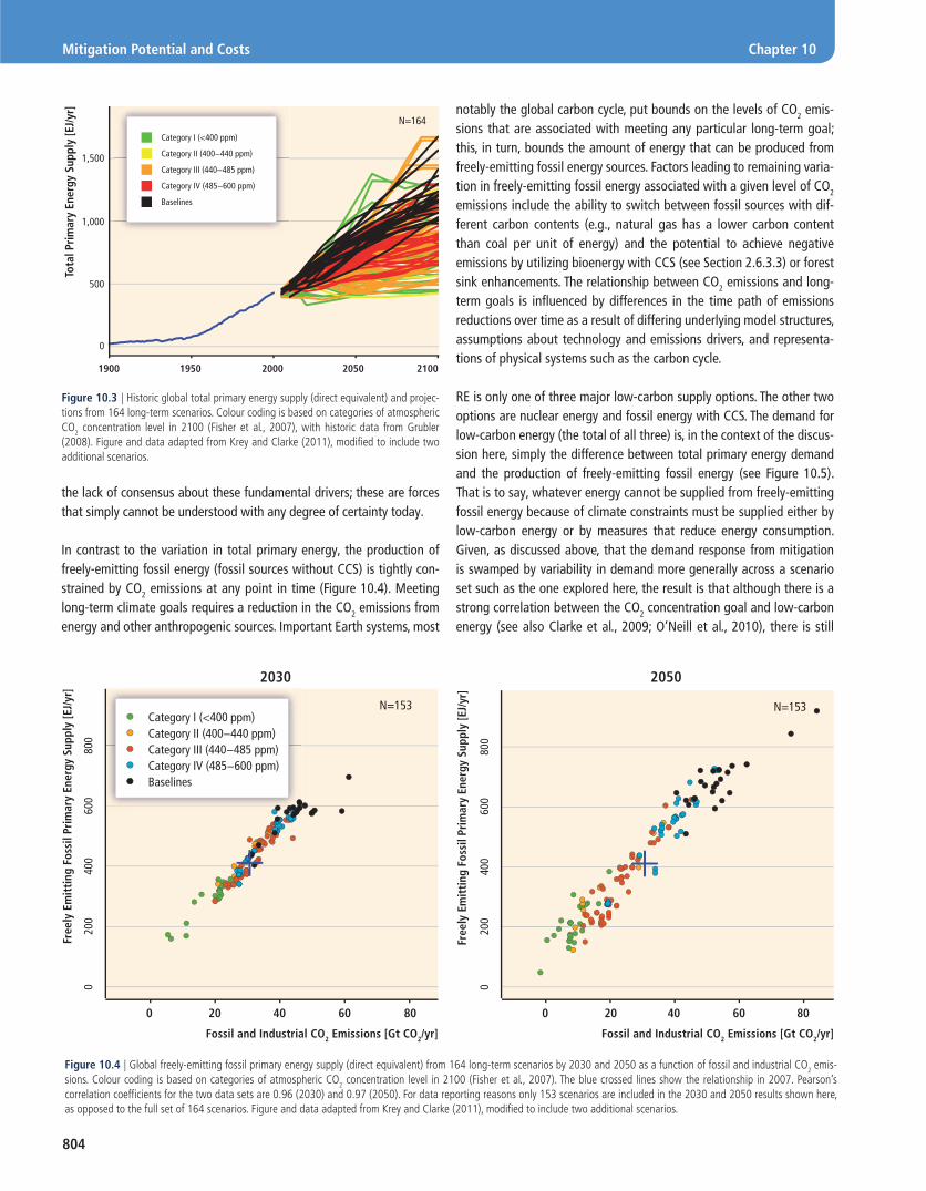
notably the global carbon cycle, put bounds on the levels of CO2 emis-sions that are associated with meeting any particular long-term goal; this, in turn, bounds the amount of energy that can be produced from freely-emitting fossil energy sources. Factors leading to remaining varia-tion in freely-emitting fossil energy associated with a given level of CO2 emissions include the ability to switch between fossil sources with dif-ferent carbon contents (e.g., natural gas has a lower carbon content than coal per unit of energy) and the potential to achieve negative emissions by utilizing bioenergy with CCS (see Section 2.6.3.3) or forest sink enhancements. The relationship between CO2 emissions and long-term goals is infl uenced by differences in the time path of emissions reductions over time as a result of differing underlying model structures, assumptions about technology and emissions drivers, and representa-tions of physical systems such as the carbon cycle.

RE is only one of three major low-carbon supply options. The other two options are nuclear energy and fossil energy with CCS. The demand for low-carbon energy (the total of all three) is, in the context of the discus-sion here, simply the difference between total primary energy demand and the production of freely-emitting fossil energy (see Figure 10.5). That is to say, whatever energy cannot be supplied from freely-emitting fossil energy because of climate constraints must be supplied either by low-carbon energy or by measures that reduce energy consumption. Given, as discussed above, that the demand response from mitigation is swamped by variability in demand more generally across a scenario set such as the one explored here, the result is that although there is a strong correlation between the CO2 concentration goal and low-carbon energy (see also Clarke et al., 2009; O’Neill et al., 2010), there is still

the lack of consensus about these fundamental drivers; these are forces that simply cannot be understood with any degree of certainty today.

In contrast to the variation in total primary energy, the production of freely-emitting fossil energy (fossil sources without CCS) is tightly con-strained by CO2 emissions at any point in time (Figure 10.4). Meeting long-term climate goals requires a reduction in the CO2 emissions from energy and other anthropogenic sources. Important Earth systems, most

N=164

Tota

l Pri

mar

y En

ergy

Sup

ply

[EJ/

yr]

0

1900 1950 2000 2050 2100

500

1,000

1,500


Category II (400−440 ppm)

Category III (440−485 ppm)

Category IV (485−600 ppm)

Baselines

Figure 10.3 | Historic global total primary energy supply (direct equivalent) and projec-tions from 164 long-term scenarios. Colour coding is based on categories of atmospheric CO2 concentration level in 2100 (Fisher et al., 2007), with historic data from Grubler (2008). Figure and data adapted from Krey and Clarke (2011), modifi ed to include two additional scenarios.

0

20 40 60 800

200

400

600

800

0

200

400

600

800

20 40 60 800

2030

Fossil and Industrial CO2 Emissions [Gt CO2/yr]

Free

ly E

mit

ting

Fos

sil P

rim

ary

Ener

gy S

uppl

y [E

J/yr

]

N=153Category I (<400 ppm)Category II (400−440 ppm)Category III (440−485 ppm)Category IV (485−600 ppm)Baselines

2050


Free

ly E

mit

ting

Fos

sil P

rim

ary

Ener

gy S

uppl

y [E

J/yr

]

N=153

Figure 10.4 | Global freely-emitting fossil primary energy supply (direct equivalent) from 164 long-term scenarios by 2030 and 2050 as a function of fossil and industrial CO2 emis-sions. Colour coding is based on categories of atmospheric CO2 concentration level in 2100 (Fisher et al., 2007). The blue crossed lines show the relationship in 2007. Pearson’s correlation coeffi cients for the two data sets are 0.96 (2030) and 0.97 (2050). For data reporting reasons only 153 scenarios are included in the 2030 and 2050 results shown here, as opposed to the full set of 164 scenarios. Figure and data adapted from Krey and Clarke (2011), modifi ed to include two additional scenarios.

805


N=164

200

400

600

800

0

200

400

600

800

0

20 40 60 80020 40 60 800

2030


Low

−Ca

rbon

Pri

mar

y En

ergy

Sup

ply

[EJ/

yr]

N=161Category I (<400 ppm)Category II (400−440 ppm)Category III (440−485 ppm)Category IV (485−600 ppm)Baselines

2050


Low

−Ca

rbon

Pri

mar

y En

ergy

Sup

ply

[EJ/

yr]

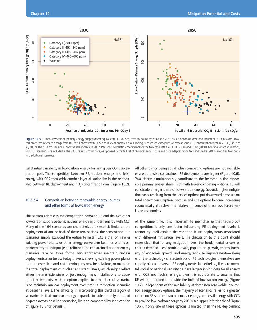
Figure 10.5 | Global low-carbon primary energy supply (direct equivalent) in 164 long-term scenarios by 2030 and 2050 as a function of fossil and industrial CO2 emissions. Low-carbon energy refers to energy from RE, fossil energy with CCS, and nuclear energy. Colour coding is based on categories of atmospheric CO2 concentration level in 2100 (Fisher et al., 2007). The blue crossed lines show the relationship in 2007. Pearson’s correlation coeffi cients for the two data sets are -0.60 (2030) and -0.68 (2050). For data reporting reasons, only 161 scenarios are included in the 2030 results shown here, as opposed to the full set of 164 scenarios. Figure and data adapted from Krey and Clarke (2011), modifi ed to include two additional scenarios.

substantial variability in low-carbon energy for any given CO2 concen-tration goal. The competition between RE, nuclear energy and fossil energy with CCS then adds another layer of variability in the relation-ship between RE deployment and CO2 concentration goal (Figure 10.2).

10.2.2.4 Competition between renewable energy sources and other forms of low-carbon energy

This section addresses the competition between RE and the two other low-carbon supply options: nuclear energy and fossil energy with CCS. Many of the 164 scenarios are characterized by explicit limits on the deployment of one or both of these two options. The constrained CCS scenarios simply excluded the option to install CCS either on new or existing power plants or other energy conversion facilities with fossil or bioenergy as an input (e.g., refi ning). The constrained nuclear energy scenarios take on three forms. Two approaches maintain nuclear deployments at or below today’s levels, allowing existing power plants to retire over time and not allowing any new installations, or maintain the total deployment of nuclear at current levels, which might refl ect either lifetime extensions or just enough new installations to coun-teract retirements. A third option applied in a number of scenarios is to maintain nuclear deployment over time in mitigation scenarios at baseline levels. The diffi culty in interpreting this third category of scenarios is that nuclear energy expands to substantially different degrees across baseline scenarios, limiting comparability (see caption of Figure 10.6 for details).

All other things being equal, when competing options are not available or are otherwise constrained, RE deployments are higher (Figure 10.6). Two effects simultaneously contribute to the increase in the renew-able primary energy share. First, with fewer competing options, RE will constitute a larger share of low-carbon energy. Second, higher mitiga-tion costs resulting from the lack of options put downward pressure on total energy consumption, because end-use options become increasing economically attractive. The relative infl uence of these two forces var-ies across models.

At the same time, it is important to reemphasize that technology competition is only one factor infl uencing RE deployment levels; it cannot by itself explain the variation in RE deployments associated with different mitigation levels. The discussion to this point should make clear that for any mitigation level, the fundamental drivers of energy demand—economic growth, population growth, energy inten-sity of economic growth and energy end-use improvements—along with the technology characteristics of RE technologies themselves are equally critical drivers of RE deployments. Nonetheless, if environmen-tal, social or national security barriers largely inhibit both fossil energy with CCS and nuclear energy, then it is appropriate to assume that RE will be required to provide the bulk of low-carbon energy (Figure 10.7). Independent of the availability of these non-renewable low-car-bon energy supply options, the majority of scenarios relies to a greater extent on RE sources than on nuclear energy and fossil energy with CCS to provide low-carbon energy by 2050 (see upper left triangle of Figure 10.7). If only one of these options is limited, then the RE deployment

806


0

10

20

30

40

50

450 ppmv

CO2

450 ppmv

CO2

450 ppmv

CO2

400 ppmv

CO2 eq (*)

550 ppmv

CO2 eq

400 ppmv

CO2 eq (*)

550 ppmv

CO2 eq

400 ppmv

CO2 eq (*)

550 ppmv

CO2 eq

450 ppmv

CO2 eq

550 ppmv

CO2 eq

550 ppmv

CO2 eq (*)

ReMIND (ADAM)POLES (ADAM)MERGE-ETL (ADAM)MESSAGE (EMF22)DNE21+ WITCH(RECIPE)

IMACLIM(RECIPE)

ReMIND(RECIPE)

No CCS & Limited Nuclear

Limited Nuclear

No CCS

Standard

Add

itio

nal R

enew

able

Pri

mar

y En

ergy

Sha

re[P

erce

ntag

e Po

ints

Cha

nge

Rela

tive

to

Base

line]

Not

Eva

luat

ed

Not

Eva

luat

ed

Not

Eva

luat

ed

Not

Eva

luat

ed

Not

Eva

luat

ed

Not

Eva

luat

ed

Not

Eva

luat

ed

XNot

Eva

luat

ed

Figure 10.6 | Increase in global renewable primary energy share (direct equivalent) in 2050 in selected constrained technology scenarios compared to the respective baseline sce-narios. The ‘X’ indicates that the respective concentration level for the scenario was not achieved. The defi nition of ‘Limited Nuclear’ and ‘No CCS’ cases varies across models. The DNE21+, MERGE-ETL and POLES scenarios represent nuclear phase-outs at different speeds; the MESSAGE scenarios limit the deployment to 2010; and the ReMIND, IMACLIM and WITCH scenarios limit nuclear energy to the contribution in the respective baseline scenarios, which can still imply a signifi cant expansion compared to current deployment levels. The REMIND (ADAM) 400 ppm no CCS scenario refers to a scenario in which cumulative CO2 storage is constrained to 120 Gt CO2, The MERGE-ETL 400 ppm no CCS case allows cumulative CO2 storage of about 720 Gt CO2. The POLES 400 ppm CO2eq no CCS scenario was infeasible and therefore the respective concentration level of the scenario shown here was relaxed by approximately 50 ppm CO2. The DNE21+ scenario is approximated at 550 ppm CO2eq based on emissions pathways through 2050. Figure adapted from Krey and Clarke (2011).

proportions of low-carbon energy are generally higher than they would otherwise be, but the degree of this effect is dependent on the abil-ity of the other of these options to take up the slack in lieu of RE. In many modelling paradigms, fossil energy with CCS and nuclear energy are assumed to be close substitutes for the production of base-load electricity production. When one is not available, the majority of the generation it would have provided is provided instead by the other rather than by RE sources, because solar, wave and wind energy are variable. At the same time, it is important to note that reservoir hydro-power, bioenergy and geothermal energy can be dispatchable base load (Section 8.2.1).

A fundamental question raised by limited technology scenarios is whether one or more energy supply options are ‘necessary’ this century to meet low stabilization goals; that is, could the goal still be met if these technologies were not available. One way to explore this issue is to identify scenarios that were attempted with limited technology, but that could not be produced by the associated models. These attempts give a sense of the diffi culty of meeting stabilization goals with limited technology options, although, in most cases, they cannot truly be con-sidered as indications of physical feasibility (Clarke et al., 2009). These attempted scenarios tell a mixed story. In some cases, models could not achieve stabilization without nuclear and CCS; however, in others, mod-els were able to produce these scenarios (Figure 10.6). Several studies found that limits on RE deployments kept models from achieving stabili-zation goals (see, e.g., Figure 10.11). Other studies have indicated that it is the combination of RE, in the form of bioenergy, with CCS that makes

low stabilization goals substantially easier through negative emissions (Azar et al., 2006; van Vuuren et al., 2007; Clarke et al., 2009; Edenhofer et al., 2010; Tavoni and Tol, 2010).

10.2.2.5 Renewable energy deployment by technology, over time and by region

There is great variation in the deployment characteristics of individ-ual technologies (Figures 10.8 and 10.9). Several dimensions of this variation bear mention. First, the absolute scales of deployments vary considerably among technologies. Bioenergy, wind and solar energy generally show higher incremental deployment levels than hydropower and geothermal energy, although the variation is large enough that there are clearly scenarios with minimal penetration of wind and solar relative to hydropower and geothermal energy. Ocean energy is cur-rently only represented in very few scenarios and will therefore not be discussed here (see also Section 10.2.4). Further, deployment mag-nitudes are characterized by greater variation for some technologies relative to others. For example, variation in hydroelectric deployment is far less than in geothermal deployment. The high deployment sce-narios for geothermal energy probably assume competitive electricity from enhanced geothermal systems and/or wide application of geo-thermal heat pumps (see Sections 4.2 and 4.8). It is important to use some caution in interpreting the bioenergy numbers in Figures 10.8 and 10.9 relative to those associated with the other renewable energy tech-nologies. This analysis is being conducted using the direct equivalent

807


Figure 10.7 | Global RE primary energy supply (direct equivalent) plotted against non-renewable low-carbon energy primary energy supply (direct equivalent) in 2030 and 2050. Colour coding is based on categories of atmospheric CO2 concentration level in 2100 (Fisher et al., 2007). The shapes identify constraints on the availability of the competing low-carbon energy supply options, fossil with CCS and nuclear. Note that limited nuclear scenarios include nuclear phase-outs, constraints on the production of new nuclear energy and scenarios in which nuclear production is constrained to baseline levels. The blue crossed lines show the relationship in 2007. For data reporting reasons, only 152 and 155 scenarios are included in the 2030 and 2050 results shown here, as opposed to the full set of 164 scenarios. Figure and data adapted from Krey and Clarke (2011), modifi ed to include two additional scenarios.

050

100

150

200

250

300

2030

N=152

Non-Renewable Low-Carbon Primary Energy Supply [EJ/yr]

Rene

wab

le P

rim

ary

Ener

gy S

uppl

y [E

J/yr

]

0 10050 150 250200 300

010

020

030

040

050

0

2050

N=155

CCS and NuclearNoCCS and NuclearCCS and LimNuclearNoCCS and LimNuclear

Non-Renewable Low-Carbon Primary Energy Supply [EJ/yr]

Rene

wab

le P

rim

ary

Ener

gy S

uppl

y [E

J/yr

]

0 100 200 300 400 500

Category I (<400 ppm)Category II (400−440 ppm)Category III (440−485 ppm)Category IV (485−600 ppm)Baselines

they were to be converted to primary energy by using the substitution method, then they might be roughly three times larger, based on aver-age fossil electricity effi ciencies.

Second, the time scale of deployment varies across different RE tech-nologies (Figures 10.8 and 10.9), in large part representing differences in deployment levels today and (often) associated assumptions about relative technological maturity. For example, hydroelectric power experi-ences only modest growth across scenarios (a 1.7-fold increase in the median case and a 3-fold increase in the highest scenario by 2050 com-pared to today); wind energy grows more rapidly, beginning from lower deployment levels today; and solar energy grows most rapidly, begin-ning from only minimal deployment today, as well as in 2020 in most scenarios. Indeed, much of the growth in solar energy occurs after 2030, indicating a general consistency among scenarios that solar energy at a large scale is a longer-term option than several other options. Global bioenergy production includes both traditional uses of biomass (more than 30 EJ/yr or roughly two-thirds of all bioenergy consumption in 2008, see Chapter 2) as well as more advanced methods, including cellulosic approaches. Traditional biomass use is typically assumed to decline as economic development progresses, implying that the growth in bioenergy is largely in modern applications. It is also useful to note that some technologies appear to be more clearly infl uenced by the cli-mate policy than others. For example, solar energy deployment levels are noticeably higher in the most ambitious climate scenarios than in the other scenarios. All of the technologies experience this effect but to varying degrees.

Finally, scenarios generally indicate that RE deployment is larger in non-Annex I countries over time than in the Annex I countries (Figure 10.8 and Krey and Clarke, 2011). Virtually all scenarios include the assumption that economic and energy demand growth will be larger in the non-Annex I countries than in the Annex I countries (Clarke et al., 2007, 2009). The result is that the non-Annex I countries account for an increasingly large proportion of CO2 emissions in baseline, or no-policy, cases and must therefore make larger emissions reductions over time. All other things being equal, larger reductions imply larger deployment of low-carbon supply options, including RE. Hence, it is not surprising that scenarios generally indicate larger RE deployment levels in non-Annex I regions.

At the same time, it is important to note that the actual deployment lev-els, particularly in the nearer term, will depend not only on the long-term

accounting method. Bioenergy is accounted for prior to conversion to fuels such as ethanol or electricity when it is used in those applica-tions. In contrast, the other technologies generally produce electricity, and they are accounted for as electricity produced in these cases. If

808


goal, but also on the degree to which countries take action towards the long-term goal. For example, in scenarios in which some countries delay participation in global emissions reductions, RE deployment is neces-sarily lower than it is in scenarios with full global participation (Clarke et al., 2009; Krey and Clarke, 2011). Nonetheless, because stabilization of CO2 concentrations means bringing CO2 emissions to near zero, all

2030

AI NAI AI NAI AI NAI AI NAI AI NAI

[EJ/

yr]

0

50

100

150

200

2050

[EJ/

yr]

0

50

100

150

200

AI NAI AI NAI AI NAI AI NAI AI NAI

Bioenergy

Hydropower

Wind Energy

Direct Solar Energy

Geothermal Energy

Maximum

75th Percentile

Median

25th Percentile

Minimum

Figure 10.8 | Global RE primary energy supply (direct equivalent) by source in Annex I (AI) and Non-Annex I (NAI) countries in 164 long-term scenarios by 2030 and 2050. The thick black line corresponds to the median, the coloured box corresponds to the inter-quartile range (25th to 75th percentile) and the ends of the white surrounding bars correspond to the total range across all reviewed scenarios. Depending on the source, the number of scenarios underlying these fi gures varies between 122 and 164. Note that ocean energy is represented in very few scenarios, insuffi cient to generate a similar graph. Although instructive for interpreting the information, it is important to note that the 164 scenarios are not explicitly a random sample meant for formal statistical analysis. (One reason that bioenergy supply appears larger than supplies from other sources is that the direct equivalent method is used to represent primary energy in this fi gure. Bioenergy is accounted for prior to conversion to fuels such as ethanol or electricity. The other tech-nologies produce primarily (but not entirely) electricity and they are accounted for based on the electricity produced. If primary equivalents were used, based on the substitution method, rather than direct equivalents, then energy production from non-biomass renew-able sources would be of the order of three times larger than shown here.) Figure and data adapted from Krey and Clarke (2011), modifi ed to include two additional scenarios.

countries must eventually bring their emissions to this point, and those with larger energy consumption will require more low-carbon energy than others, regardless of which countries may have initiated action on climate the soonest. It is also important to note that countries may take different approaches to mitigation, some focusing on price-based poli-cies where others use regulatory policies that could include mandates for RE, and this could infl uence the spatial character of RE deployments. The scenarios described here mostly rely exclusively on price-based miti-gation and therefore do not capture this sort of variation.

10.2.2.6 Renewable energy and the costs of mitigation

RE’s role in climate mitigation might be observed not only through the lens of RE deployment levels, but also by an exploration of the man-ner in which RE availability and deployment infl uences the economic consequences, or costs, of mitigation. One way that researchers have attempted to link particular technologies to mitigation costs is to build mitigation cost curves; that is, relationships that indicate how much mit-igation might be achieved by particular technologies at a given carbon price. In the context of RE, these curves attempt to answer the question: how much CO2 abatement and at what cost can be provided by RE tech-nologies? Such mitigation cost curves are not provided here for reasons discussed more thoroughly in Section 10.4. It is noted here only that assigning mitigation to particular technologies is not a primary output of integrated models. Integrated models provide information on prices, emissions and deployments, but in general they do not assign emissions to the presence or absence of specifi c technologies. Such assignments are the result of post-processing, offl ine accounting calculations that rely on analyst judgment about key assumptions. Applying these post-processing assumptions to the scenarios would constitute new analysis rather than synthesis, and it would blur the signal from the scenarios themselves. A sense of the variation of CO2 emission mitigation due to the use of different methods is given in Section 10.3 on the basis of 4 selected scenarios from the whole set of 164 analyzed in this section. In addition, these analyses do not account for the benefi ts of climate mitigation (e.g., less severe climate change impacts in the long term, reduced need for adaptation), secure energy supply and air pollution

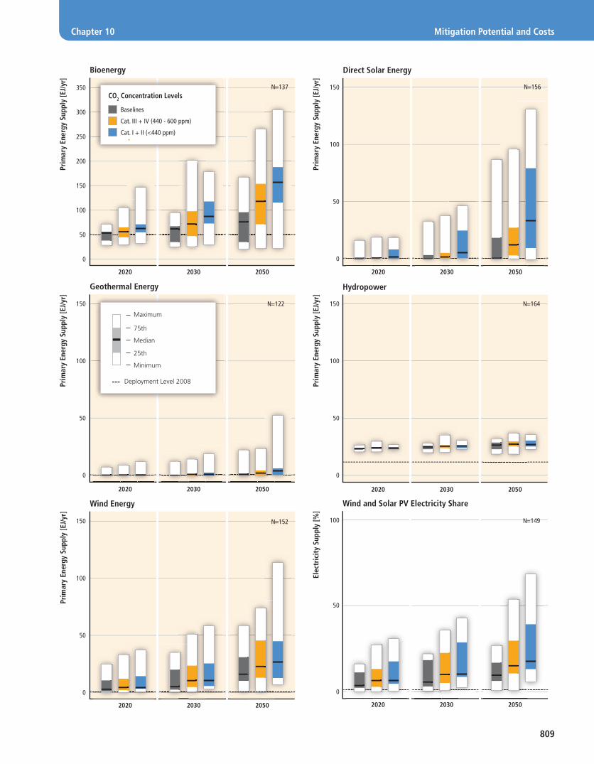
809


Deployment Level 2008

Maximum

75th

Median

25th

Minimum

CO2 Concentration Levels

Direct Solar Energy

Geothermal Energy

Wind Energy

Hydropower

Wind and Solar PV Electricity Share

Prim

ary

Ener

gy S

uppl

y [E

J/yr

]Pr

imar

y En

ergy

Sup

ply

[EJ/

yr]

Prim

ary

Ener

gy S

uppl

y [E

J/yr

]Pr

imar

y En

ergy

Sup

ply

[EJ/

yr]

Prim

ary

Ener

gy S

uppl

y [E

J/yr

]

Elec

tric

ity

Supp

ly [%

]

2020 20502030 2020 20502030

2020 20502030

2020 20502030

2020 20502030

2020 20502030

0

50

150

100

0

50

150

100

0

0

50

150

100

0

50

150

100

0

50

100

Bioenergy

50

150

100

Baselines

Cat. III + IV (440 - 600 ppm)

Cat. I + II (<440 ppm)

200

250

300

350

N=122

N=137 N=156

N=164

N=149N=152

810


2050

Renewable Primary Energy Supply [EJ/yr]

Carb

on P

rice

[USD

/t C

O2]

0 100 200 300 400 500

050

01,

000

1,50

0

N=141

Category I (<400 ppm)Category II (400−440 ppm)Category III (440−485 ppm)Category IV (485−600 ppm)Baselines

CCS and NuclearNoCCS and NuclearCCS and LimNuclearNoCCS and LimNuclear

Figure 10.10 | Carbon prices (in USD2005) as a function of global RE primary energy sup-ply (direct equivalent) in 2050. Colour coding is based on categories of atmospheric CO2 concentration level in 2100 (Fisher et al., 2007). Different symbols in the graph denote the availability of CCS and nuclear energy. Note that limited nuclear scenarios include nuclear phase-outs, constraints on the production of new nuclear and scenarios in which nuclear production is constrained to baseline levels. For data reporting reasons, only 141 scenarios are included in the 2050 results shown here, as opposed to the full set of 164 scenarios. Figure and data adapted from Krey and Clarke (2011), modifi ed to include two additional scenarios.

Figure 10.9 | (Preceding page) Global primary energy supply (direct equivalent) of biomass, wind, solar, hydro, and geothermal energy and share of variable RE (wind and solar photovoltaic) in global electricity generation in 164 long-term scenarios in 2020, 2030 and 2050, and grouped by different categories of atmospheric CO2 concentration level in 2100 (Fisher et al., 2007). Following the direct equivalent methodology, biomass primary energy supply is accounted for prior to conversion whereas the other RE options are accounted for based on secondary energy produced. The thick black line corresponds to the median, the coloured box corresponds to the inter-quartile range (25th to 75th percentile) and the ends of the white surrounding bars correspond to the total range across all reviewed scenarios. Although instructive for interpreting the information, it is important to note that the 164 scenarios are not explicitly a random sample meant for formal statistical analysis. For data reporting reasons, the number of scenarios included in each of the panels shown here varies considerably. The number of scenarios (N) underlying the individual panels, as opposed to the full set of 164 scenarios, is indicated in the right upper corner of each panel. Figure and data adapted from Krey and Clarke (2011), modifi ed to include two additional scenarios.

assumptions about the availability or cost and performance of RE as well as competing mitigation options. A number of researchers have explored this issue (see, e.g., Clarke et al., 2008; Luderer et al., 2009; Edenhofer et al., 2010; Tavoni and Tol, 2010). Consistent with intuition, these studies demonstrate that the presence of RE technologies or improvements in the cost and performance of RE technologies reduces mitigation costs. This is not surprising: more or better options should not increase costs. More important is the relative magnitude of the change in mitigation costs resulting from increases in the availability, cost or performance of RE technologies relative to the change in mitigation costs resulting from

(e.g., reduced health expenditures) due to the deployment of RE tech-nologies (see e.g., Nemet et al., 2010). A more detailed discussion of co-benefi ts can be found in Section 10.6.

Another possible view into the relationship between RE and mitigation costs is afforded by considering the relationship between RE deploy-ment levels and carbon prices across scenarios. This approach attempts to answer the question: how much RE will be deployed at a given car-bon price? The 164 scenarios demonstrate no meaningful correlation between RE deployment and carbon prices (see Figure 10.10). All the forces that blur the relationship between RE deployment levels and long-term concentration goals, as discussed in Sections 10.2.2.2, 10.2.2.3 and 10.2.2.4, infl uence the relationship between RE deployment and carbon prices. In addition, integrated energy models are characterized by a wide range of carbon prices based both on parameter assumptions and model structure (Clarke et al., 2007, 2009). The result is little ability to link RE deployment levels to carbon prices when looking across a wide range of models.

CO2 prices are only a limited metric for cost because they represent the marginal costs of abatement and not the total cost. A range of other cost measures have been used in the literature to capture the economic consequences of mitigation. These include changes in gross domestic product (GDP) or consumption, or total mitigation costs, that is, the addi-tional cost to deploy and operate an energy system with lower GHG emissions, which can provide a broader sense of the cost implications of RE. In general, mitigation tends to reduce GDP (Fisher et al., 2007).3

However, these measures do not necessarily lead to a stronger correla-tion with RE deployment than carbon prices. For example, the overall variation of GDP in the baseline scenarios reviewed in this section (a factor of 1.8 in 2050 between the lowest and the highest GDP) is much larger than the changes in GDP as the result of climate mitigation (up to a few percent of baseline GDP by 2050), which can be derived by com-paring the GDP in mitigation scenarios to their respective baseline for those models that include feedbacks to GDP. The dominance of, and vari-ation in, baseline GDP would further obscure any relationship between total GDP and RE deployment.

A different refl ection of the relationship between the economic con-sequences of mitigation and RE deployments can be ascertained by exploring how mitigation costs would change under differing

3 Note that a minority of researchers have argued that climate mitigation could lead to increased economic output (e.g., Barker et al., 2006). The basic argument is that under specifi c assumptions, induced technological change due to a carbon price increase leads to additional investments that trigger higher economic growth.

811


increases in the availability of fossil energy with CCS and/or nuclear energy. For example, in both the ADAM (Edenhofer et al., 2010) and RECIPE projects (Luderer et al., 2009), each involving three models, the cost increase that results from the absence of the option to expand RE deployment is not of a distinctly different order of magnitude than the cost increase from the absence of the option to implement fossil energy with CCS or expand production of nuclear energy beyond today’s lev-els or beyond baseline levels (see Figures 10.11 and 10.12). Indeed, in several scenarios, constraining RE results in larger cost increases than constraining nuclear power or fossil energy with CCS. The value

of RE availability, cost and performance may also vary with the degree of ambition. For example, the availability of bioenergy with CCS has been identifi ed as a particularly valuable technology combination for meeting tight stabilization constraints (Azar et al., 2006; van Vuuren et al., 2007; Clarke et al., 2009; Edenhofer et al., 2010; Tavoni and Tol, 2010). To summarize, while there is an agreement in the literature that mitigation costs will increase if the deployment of RE technologies is constrained and that more ambitious stabilization levels may not be reachable, there is little agreement on the precise magnitude of the cost increase.

Biomax

All Options

No Nuclear

Biomin

No CCS

No RE

Biomax

All Options

No Nuclear

Biomin

No CCS

No RE

XX XX XXX

6

5

4

3

2

1

0

6

5

4

3

2

1

0

6

5

4

3

2

1

0

6

5

4

3

2

1

0

Mit

igat

ion

Cost

[%G

DP]

Mit

igat

ion

Cost

[%G

DP]

Aba

tem

ent

Cost

s [%

GD

P]

Aba

tem

ent

Cost

s [%

GD

P]

MERGE ReMIND POLES MERGE ReMIND POLES

Mitigation Costs, World 400ppmMitigation Costs, World, 550ppm

Figure 10.11 | Global mitigation costs from the ADAM project under varying assumptions regarding technology availability for long-term stabilization levels of 550 and 400 ppm CO2eq (Edenhofer et al., 2010). Mitigation costs are given as aggregated GDP losses (MERGE, REMIND) or increase of abatement costs (POLES) up to 2100 relative to baseline in % of GDP. ‘All Options’ refers to the standard technology portfolio assumptions in the different models, while ‘Biomax’ and ‘Biomin’ assume double and half the standard technical potential of biomass of 200 EJ, respectively. ‘No CCS’ excludes CCS from the mitigation portfolio and ‘No Nuclear’ and ’No RE’ constrain the deployment levels of nuclear and RE to the baseline level, which still potentially means a considerable expansion compared to today. The ‘x’ in the right panel indicates non-attainability of the 400 ppm CO2eq level in the case of limited technology options.

Figure 10.12 | Mitigation costs from the RECIPE project under varying assumptions regarding technology availability for a long-term stabilization level of 450 ppm CO2 (Luderer et al., 2009). Option values of technologies in terms of consumption losses for scenarios in which the option indicated is foregone (CCS) or limited to baseline levels (all other technologies) for the periods (a) 2005 to 2030 and (b) 2005 to 2100. Option values are calculated as differences in consumption losses for a scenario in which the use of certain technologies is limited with respect to the baseline scenario. Note that for WITCH, the generic backstop technology was assumed to be unavailable in the ‘Fix RE’ scenario.

450 ppm C&C

Fix Nuclear

Fix Biomass

No CCS

Fix RE

No CCS, Fix Nuclear

(a) Global, 2005–2030

Cons

umpt

ion

Loss

es [%

]

Cons

umpt

ion

Loss

es [%

]

0

1

2

3

4

IMACLIM-R ReMIND-R WITCHIMACLIM-R ReMIND-R WITCH

(b) Global, 2005–2100

0

1

2

3

4

812


10.2.3 The deployment of renewable energy sources in scenarios from the technology perspective

The scenarios in this section were produced using global, integrated models. These models have several advantages, but they also have the weakness that they pay only limited attention to many critical factors that ultimately will infl uence the deployment of RE. As a means to bet-ter understand the role of these forces, the scenarios from this section are briefl y explored in the ‘long-term deployment in the context of carbon mitigation’ sections of Chapters 2 through 7. The aim of these individual technology explorations is to identify potential barriers that an expansion of RE may face and enabling factors to achieve the higher RE deployments levels as found in the scenario literature. This section briefl y summarizes the key elements of those sections.

Resource Potential: In general, even the highest deployment levels were not considered to be constrained by the available technical poten-tials at the global level for all of the RE categories. However, because RE resources are regionally heterogeneous, some of the higher deployment levels may begin to constrain the economically most attractive sites, for example, for hydro and wind energy. For most RE sources, availability is geographically constrained, for example, for certain forms of ocean, geothermal, biomass and solar energy, as well as hydropower and wind energy. In the case of bioenergy, the supply levels in the scenarios with low GHG stabilization levels of up to about 300 EJ/yr by 2050 almost exactly coincide with the upper range of possible deployment levels as discussed in Chapter 2 (see Section 2.8.4 and Figure 2.8.3).

Regional Deployment: Economic development and technology matu-rity are primary determinants of regional deployment levels. Regional policy frameworks for RE need to be economically attractive and pre-dictable. For mature technologies such as large hydropower, a large fraction of available technical potential in Organisation for Economic Cooperation and Development (OECD) countries has been exhausted and the largest future expansion is expected in the non-OECD countries of Asia and Latin America. For wind energy, which has seen high expan-sion rates, mostly in Europe and North America over the past decade as well as in China and India more recently, a greater geographical distri-bution of deployment than currently observed is likely to be needed to achieve the higher deployments indicated by the scenario literature. The other, less mature technologies are likely to initially focus on expansion in affl uent regions (Europe, North America, Australia and parts of Asia) where fi nancing conditions and infrastructure integration are favourable.

Supply Chain Issues: In general, no insurmountable medium- to long-term constraints of materials, labour and manufacturing capacity were identifi ed that would prevent higher deployment levels in the scenar-ios. For example, the wind industry has witnessed rapid expansion over the past that led to globalization of the production chain, but further scaling up of the industry will be needed to reach the capacity addi-tion rates seen in the more stringent scenarios. It is also important to recognize that markets and supply chains for some technologies are

global (e.g., wind, solar photovoltaic (PV)) while others (e.g., passive solar and low-temperature solar thermal) to date are largely local. As markets expand, they are likely to become more global in scope. Past rates of growth suggest that, assuming that policy and market signals are clear, no absolute long-term constraints exist.

Technology and Economics: Because the maturity of the renewable technologies is highly variable, so is the need for cost and technological advances. On the one end of the spectrum, hydropower is competitive with thermal power plants, while on the other end of the spectrum, commercial-scale demonstration plants for most ocean energy technol-ogies do not yet exist. For offshore wind energy, more remote offshore locations will require further technology advances; further, cost reduc-tions will impact deployment outcomes. Similarly, concentrating solar power (CSP), solar PV, geothermal heat pumps, and enhanced geo-thermal systems (EGS) will require technological improvements, but in particular further reductions in electricity generation costs. Technical progress is similarly required for advanced biofuels and bio-refi neries with potential for commercialization around 2020 given R&D invest-ment and near-market support.

Systems Integration and Infrastructure: Systems integration is chal-lenging for the variable electricity generation technologies wind, solar PV and wave energy (Section 8.2.1). Technical (e.g., balancing gen-eration capacity, inter-connection and storage) and institutional (e.g., market design and operations, market access and tariff structure) solu-tions will need to be implemented to address operational integration concerns. Additionally, substantial new transmission infrastructure may be required under even modest expansion scenarios to connect remote resources, for example, off- but also onshore wind power, central station CSP and PV, hydrothermal geothermal power and hydropower. A greater reliance on offshore wind power is likely for regions such as Europe, which will require the development of offshore transmission infrastruc-ture; certain forms of ocean energy face similar integration challenges and synergies may therefore exist in the deployment of these technolo-gies. To gain greater penetration into the energy supply systems, other RE-based energy carriers such as heat, biogas, liquid bio-fuels, solid bio-mass and hydrogen all need appropriate integration into existing system infrastructure as outlined in Section 8.2.

10.2.4 Knowledge gaps

The primary knowledge gap with respect to the assessment of RE in large-scale, integrated models is the representation of RE technolo-gies themselves within these models. The coverage of different RE sources in the scenario literature varies signifi cantly. Mature technolo-gies such hydropower were included by all models reviewed in this assessment, while less mature technologies or those not deployed today at large scale—for example, ocean energy, offshore wind, con-centrating solar power and geothermal energy—were addressed by smaller sets of scenarios. One reason is that there is less demand to

813


specifi cally address less mature technologies or those that are a priori assumed to have lower contributions. A second reason is that there is a lack of high-quality global resource data (preferably gridded) for some renewable resources (e.g., geothermal energy, the various ocean energy forms), which is a precondition for constructing resource supply curves that are inputs to energy-economic and integrated assessment models. More broadly, beyond representations of the technologies themselves, many issues related the implementation of RE technolo-gies require further research and inclusion in large-scale integrated models. Important areas in this regard include the integration of RE into the electricity grid and the relationship between bioenergy pro-duction, crop production and deforestation.

However, it is important to note that improved representations of RE technologies and associated systems will not entirely eliminate the uncertainty regarding the role of RE in climate mitigation. As was discussed throughout this section, a range of other uncertainties, unre-lated to RE technologies, such as economic and population growth, the availability, cost and performance of competing technologies, and the nature of mitigation approaches and ambitions will infl uence the role of RE in climate mitigation. Uncertainty derived simply from the design of different modelling platforms can also infl uence results. Therefore, an important research priority for the future is to improve the understanding of why model results vary with respect to RE and to attribute these differences in model outcomes to differences in assumptions and methodologies.

10.3 Assessment of representative mitigation scenarios for different renewable energy strategies

Section 10.2, coming from a more statistical perspective, gave a com-prehensive overview of the possible role RE technologies could play in different mitigation pathways. In contrast, this section goes beyond the more aggregated data level and focuses on regional and sectoral perspectives. For this in-depth analysis, four scenarios from the previ-ous section’s full set of the scenario assessments have been chosen to represent different illustrative energy and emission pathways (see Table 10.3). The scenarios differ in assumptions, mitigation goals and in the types of underlying models used. For a description of the scenarios and models, see Box 10.2. Primary data for this analysis go beyond what has been published to date, and were provided at special request by the scenario authors and institutions.4

4 The International Energy Agency (IEA) and the German Aerospace Center for IEA-WEO2009 Baseline; the Potsdam Institute for Climate Impact Research for ReMIND-RECIPE; the Pacifi c Northwest National Laboratory for MiniCAM-EMF22; and the German Aerospace Center for ER-2010.

10.3.1 Sectoral breakdown of renewable energy sources

The amount of RE deployed in the scenarios depends on a large num-ber of variables, assumptions and input data (see also Section 10.2.1, especially Section 10.2.1.1). Often most infl uential are the cost and performance assumptions for the different RE technologies. They help determine the comparative attractiveness of competing low-carbon supply options (i.e., nuclear energy and fossil energy with CCS), but also of end-use energy effi ciency measures. Underestimation of costs leads to overestimation of RE deployment and vice versa. The share of RE calculated is furthermore determined by the general availability of competing options. Constraints on alternative mitigation options mean that more RE deployment will occur for a given level of GHG mitigation. Assumptions about infrastructure restrictions and system integration options are further important determinants. In this context, a signifi -cant factor relates to assumptions about how the power grid would adapt to signifi cant amounts of variable renewable resources. In con-trast, the overall technical potential for RE—that is, the total amount of energy that can be produced taking into account the primary resources, the socio-geographical constraints and the technical losses in the con-version process (see defi nition in Annex I)—is not considered to be a limiting factor at the global level as the technical potential supersedes the current and projected future demand by orders of magnitude (see Section 1.2.2). Thus, to fully exploit the entire technical RE potential is neither needed nor necessary.

In practice, deployment of RE resources should respect sustainability cri-teria in order to achieve an environmentally friendly future energy supply (see Chapters 1 and 9). Public acceptance is crucial to the expansion of RE sources as well. Some RE applications, such as rooftop PV and solar thermal as well as bioenergy cogeneration plants and onshore wind, are often decentralized energy production facilities and may be located near or even at demand centres. Other RE applications are more likely to involve industrial-scale energy production facilities located at some distance from demand centres and requiring large-scale transmission, for example, large onshore wind parks, offshore wind energy, concen-trated solar power in deserts, hydrothermal geothermal plants, and hydropower. In both cases, public acceptance concerns can constrain development if not carefully managed. The use of biomass has been especially controversial recently, as issues have arisen over competition with other land uses, food production and ecosystem preservation, as well as possible direct or indirect GHG emissions due to land use change (see Sections 2.5, 9.3.4 and 10.6). On the other hand, RE deployment is positively driven by sustainability criteria since it has the potential to provide energy access in remote areas without some of the envi-ronmental and health impacts usually associated with fossil fuels (see Sections 9.3.2, 9.3.4 and 10.6). Therefore, non-economic criteria have a signifi cant infl uence on the resulting RE deployment and corresponding assumptions are crucial for scenario results.

814


Last but not least, climate and energy policy frameworks are highly relevant to RE deployment in scenario analysis. Market forces and con-straints are relevant for the deployment of RE and determine the market potential. As market potential also includes opportunities, it may in the-ory be larger than the economic potential due to support programs, but usually the market potential is lower because of a variety of constraining market failures for RE and other new technologies (Sections 1.4.2 and 11.4). Market potential analyses have to take into account the behav-iour of private economic agents under their specifi c conditions, which are partly shaped by public authorities (see Sections 11.5 and 11.6). In this context, the energy policy framework has a profound impact on the expansion of RE sources respective to corresponding assumptions for the scenario results.

RE deployment is driven and hindered by a variety of factors and very much depends on how the different determinants and their impacts are being assessed; uncertainties about future development are generally high and determined by specifi c assumptions. In this context, energy scenarios bundling a consistent set of specifi c assumptions are an approximation of what can be expected for the future under specifi c conditions. As a comparison of different scenarios spans a range of

possible futures, it can show overarching commonalities and trends and can make differences and uncertainties visible and more transparent.

Selection of four illustrative scenarios for an in-depth analysisScenario results are determined not only by parameter assumptions, but also by the underlying modelling architecture and model-specifi c restrictions (e.g., upper deployment bound for specifi c RE technologies). The four scenarios were selected to present a wide range of different modelling architectures, demand projections and technology portfolios for the supply side (see Box 10.2). The IEA-WEO2009-Baseline Reference Scenario (IEA, 2009; extension to 2050: Teske et al., 2010) (henceforth IEA-WEO2009-Baseline) is the only baseline scenario in this set, that is, it does not incorporate any climate policy targets beyond those implemented by 2009. It is characterized by a comparatively high demand projection with low RE deployment. In two of the three mitigation scenarios, ReMIND RECIPE 450 ppm Stabilization Scenario (Luderer et al., 2009) (henceforth ReMIND-RECIPE) and MiniCAM EMF 22 fi rst-best 2.6 W/m2 Overshoot Scenario (Calvin et al., 2009) (henceforth MiniCAM-EMF22), high demand expectation and a signifi cant increase in RE is combined with the pos-sibility of employing CCS and nuclear power plants. Low demand (e.g., due to a signifi cant increase in energy effi ciency) is combined with high

Table 10.3 | Overview of key parameters of the illustrative scenarios based on assumptions that are exogenous to the models’ respective endogenous model results. Dark grey marks exogenous input; dark yellow marks endogenous model results. Note that the concentration categories are defi ned in terms of CO2 (only) concentrations, while other metrics, predominantly CO2-equivalent concentrations—of Kyoto gases or of all forcing agents—are used in the literature. (Sources: IEA-WEO2009-Baseline (IEA, 2009; Teske et al., 2010), ReMIND-RECIPE (Luderer et al., 2009), MiniCAM-EMF22 (Calvin et al., 2009), ER-2010 (Teske et al., 2010)).

Category Units Status Quo BaselineCategory III+IV (440 - 600ppm)

Category I+ II (< 440ppm)

Category I+ II (< 440ppm)

Scenario name IEA-WEO2009-Baseline ReMind-RECIPE MiniCAM-EMF22 ER-2010

Model ReMind MiniCAM MESAP/PlaNet

yr 2007 2030 20501 2030 2050 2030 2050 2030 2050

Techology pathway2

Renewables all3 allsolar: PV and CSP not

differentiated

solar: PV and CSP not dif-ferentiated, ocean energy

not includedall all

CCS + + + + + + - -

Nuclear + + + + + + + -

Population billion 6.67 8.31 9.15 8.32 9.19 8.07 8.82 8.31 9.15

GDP/capita4thousand

USD2005/capita10.9 17.4 24.3 12.4 18.2 9.7 13.9 17.4 24.3

Energy Demand

(direct equivalent)EJ/y 469 645 749 590 674 608 690 474 407

Energy Intensity MJ/USD2005 6.5 4.5 3.4 5.7 4.0 7.8 5.6 3.3 1.8

Renewable Energy % 13 14 15 32 48 24 31 39 77

Fossil & Industrial

CO2 EmissionsGt CO2/y 27.4 38.5 44.3 26.6 15.8 29.9 12.4 18.4 3.7

Carbon Intensity kg CO2/GJ 58.4 57.1 56.6 45.0 23.5 49.2 18.0 36.7 7.1

Notes: 1. IEA (2009) does not cover the years 2031 until 2050. As the IEA’s projection only covers a time horizon up to 2030 for this scenario exercise, an extrapolation of the scenario has been used that was provided by the German Aerospace Agency (DLR) by extrapolating the key macroeconomic and energy indicators of WEO 2009 forward to 2050 (Teske et al., 2010). 2. (-): Technology not included; (+): Technology included. 3. This includes: Solar photovoltaics, CSP, solar water heating, wind (on- and offshore), geothermal power, heating and cogeneration, bioenergy power, heating and cogeneration, hydropower, ocean energy. 4. The data are either input for the model or endogenous model results.

815


Box 10.2 | Overview of the four illustrative scenarios and their underlying models.

IEA-WEO2009-Baseline: This scenario uses a typical baseline scenario approach. As such, it calculates the possible energy pathway without any substantial change in government policy (IEA, 2009, p. 44) and under the assumption of a minimal to moderate fossil fuel cost increase. The scenario does not include specifi c GHG emissions constraints. As the IEA (2009) projection only covers a time horizon up to 2030 for this scenario exercise, an extrapolation of the scenario has been used that was provided by the German Aerospace Center (DLR) that uses the key macroeconomic and energy indicators of IEA (2009) and brings them forward to 2050 (Teske et al., 2010). Regard-ing fossil and industrial CO2 emissions, the baseline scenario expects an increase from 27.4 Gt CO2/yr in 2007 to 44.3 Gt CO2/yr by 2050. (Scenario ‘IEA WEO 2009 Reference Scenario’ from IEA (2009) extended beyond 2030 by Teske et al. (2010).)

ReMIND-RECIPE: This scenario describes a mitigation path aiming to stabilize atmospheric CO2 (only) concentration at 450 ppm (corre-sponding to fossil and industrial CO2 emissions of 15.8 Gt CO2/yr by 2050). It was generated with the energy-economy-climate model Re-MIND-R, which computes welfare-optimized transformation trajectories under full ‘where-fl exibility’ (emission reductions are performed where it is cheapest), ‘when-fl exibility’ (emission reductions are performed when they are cheapest) and ‘what-fl exibility’ (emission reductions are performed by choosing the least expensive combination of technologies) conditions. Another crucial assumption is perfect foresight: investment decisions are made knowing in advance the future changes in prices and technology developments. The model is characterized by a high level of integration: the macro-economy and the energy system are treated within an integrated optimization framework, thus fully accounting for the macro-economic feedbacks of the climate mitigation effort. The complex integrated formulation requires compromises in terms of the sectoral and technological resolution of the energy system. ReMIND-RECIPE accounts for a variety of RE sources (wind, solar, biomass, hydro and geothermal) and conversion technologies. Wind power and solar PV are parameterized as learning technologies. RE technologies can be deployed at the industrial scale at optimal sites and be transported within world regions (up to continental scale) to demand centres, whereby the model implicitly assumes that bottlenecks (e.g., with respect to grid infrastruc-ture) are avoided by early and anticipatory planning. (Scenario ‘450 ppm stabilization scenarios’ from Luderer et al. (2009).)

MiniCAM-EMF22: The MiniCAM-EMF22 scenario was developed as part of the Energy Modelling Forum study 22 (EMF 22), which looks at possible approaches to long-term climate goals. The scenario was generated using the MiniCam integrated assessment model, the precursor to the Global Change Assessment Model (GCAM) integrated assessment model. The scenario is an overshoot scenario that reaches 450 ppm CO2eq (Kyoto gases)1 by 2100, after peaking at 525 ppm CO2eq in 2050, and assumes full international participation in emissions reductions. The specifi c concentration levels correspond with fossil and industrial CO2 emissions of 12.4 Gt CO2/yr by 2050. The underlying characteristics of the scenario include global population growth that peaks at approximately 9.0 billion people in 2070 and then declines to 8.7 billion in 2100. The scenario considers the availability of a wide range of energy supply options, including major RE options, nuclear power and both fossil energy and bioenergy equipped with CCS technology. The presence of bioenergy with CCS is par-ticularly important in the scenario because it allows for the option to create negative emissions, primarily in electricity production (Calvin et al., 2009; Clarke et al., 2009). (Scenario ‘First-best 2.6 W/m2 Overshoot Scenario’ from Calvin et al. (2009).)

ER-2010: The ER-2010 scenario (Teske et al., 2010) is based on the socioeconomic assumptions of the IEA-WEO2009-Baseline scenario, but assumes an increase in fossil fuel costs and a price for carbon from 2010 onwards. The scenario has a key constraint that limits worldwide CO2 emissions to a level of 3.7 Gt CO2 per year by 2050. To achieve this, the scenario is characterized by signifi cant efforts to fully exploit the large potential for energy effi ciency, using currently available best practice technology, and to foster the use of RE. In all sectors, the latest market development projections and the resulting cost reductions for the RE industry have been taken into account, and a stable development of the RE sector is pursued. To accelerate the market penetration of RE, various additional measures have been assumed, such as a speedier introduction of electric vehicles combined with the implementation of effective communications systems and technologies, smart meters and faster expansion of super grids to allow a higher share of variable RE power generation (PV and wind) to be employed. The methodological background of the scenario is the simulation model PlaNet of the energy and environmental planning package MESAP (see Krewitt et al. (2009), which was created for long-term strategic planning on a national, regional or local level. The model is characterized by a very detailed technology breakdown for each sector. Following the simulation approach, activities and drivers of demand (e.g., mobility demand), as well as relevant market shares of technologies, amongst other factors, are specifi ed exogenously by the user. (Scenario ‘Advanced Energy [R]evolution 2010’ from Teske et al. (2010).)

Note: 1. Note that atmospheric CO2 (only) concentrations reach about 385 ppm by 2100, that is, the scenario falls into concentration category 1 (<400 ppm); see also Table 10.2.

816


RE deployment, no employment of CCS and a global nuclear phase-out by 2045 in the third mitigation scenario, Advanced Energy [R]evolution 2010 (Teske et al., 2010) (henceforth ER-2010).

Table 10.3 shows key parameters for the four illustrative scenarios. Depending on the model, some of the assumptions may be exoge-nously applied or be determined endogenously. All scenarios project a signifi cant increase in global population and assume or calculate a signifi cant increase in GDP. The IEA-WEO2009-Baseline GDP projec-tions are based on forecasts by the International Monetary Fund (IMF, 2009) and the OECD. Those GDP projections have been used as input parameters for the ER-2010 model as well. In contrast, GDP projec-tions from MiniCAM-EMF22 and ReMIND-RECIPE are endogenously determined. Both population and GDP changes are major driving forces for future energy demand (which is endogenously calculated in all models) and therefore at least indirectly determine the resulting shares of RE.

For the set of the four illustrative scenarios, the following sections give an overview of the available data for each of the different sectors. Global energy scenarios often provide detailed information on RE elec-tricity generation. Information about the current and future RE power market is often publicly accessible, while suitable data sets about the RE heating sector and RE application in the transport sector are often not available or less detailed than for the power sector. These sectors deserve more attention, particularly because RE heating shows a sig-nifi cant technical potential and is in many cases already cost-effective (Aitken, 2003; Seyboth et al., 2007).

10.3.1.1 Renewable energy deployment in the electricity sector

The RE electricity sector scenarios analyzed here show more dynamic development and larger RE shares over the midterm compared to either the heating or transport sector scenarios.

Factors for market development in the RE electricity sectorTechnology cost and performance assumptions are among the most infl uential variables affecting energy deployment in the scenarios. The largest variations in the cost assumptions can be found for solar PV, CSP, and ocean energy. As an illustrative example: for 2020, the high-est cost projections for solar PV in the analyzed scenarios was USD2005 5,406/kW and the lowest projection was less than half of that at USD2005 2,177/kW. The upper limit is in the range of current market prices (see Section 3.8.3), although all scenarios assume cost reductions in the future. This demonstrates a typical problem in scenario analysis cover-ing a new technology market where numbers in scenarios are often superseded by recent developments. The different cost assumptions lead to very different market development pathways in the scenarios, spanning a range for solar PV-based electricity generation, even in the mitigation-oriented scenarios, from 115 TWh (414 PJ) up to 594 TWh (2,138 PJ) in 2020 (see Table 10.4), corresponding to annual market growth rates of between 18% and 42%, respectively.

However, cost projections for installed PV systems in 2050 had a signifi -cant lower level of variability, ranging from USD2005 753/kW in the low case to USD2005 1,125/kW in the high case. Nevertheless, the expected deployment rates in the scenarios are quite different. With regard to the PV-based electricity generation in 2050, there is a 25-fold differ-ence between two of the mitigation oriented scenarios: 20,790 TWh/yr (74,844 PJ/yr) in the ReMIND-RECIPE scenario versus 822 TWh/yr (2,959 PJ/yr) in MinCam-EMF22. This example illustrates the complexity of the analysis, as the resulting deployment path for PV depends not only on cost assumptions, but also on many other factors (e.g., availability and characteristics of alternative mitigation technologies like CCS and nuclear power in the case of MinCam-EMF 22).

Among all RE technologies for electricity generation, onshore wind energy saw the least variation in cost projections among the models, ranging around ±10% over the entire time frame. Cost-optimization energy models use cost assumptions for each technology as one of the main determinants of market expansion or reduction, and the input cost assumptions will therefore play a major role in determining the scenario energy mix.

Annual market potential for the RE electricity sector Based on the energy parameters of the analyzed scenarios, the required annual production capacity (representing the annual market volume) has been either calculated ex-post (IEA-WEO2009-Baseline, ReMIND-RECIPE, MinCam-EMF 22) or has been provided by the scenario authors (ER-2010). These calculated manufacturing capacities (Table 10.4) do not include the additional needs for re-powering (i.e., replacement of old wind turbines with new ones). Annual market growth rates in the analyzed scenarios are very different, as are the expectations about how the current dynamic of the market might change. In some cases, drastic reductions in the current average market growth rates have been out-lined, even in those scenarios aiming for an ambitious GHG stabilization level. The global PV industry had an average annual growth rate of 35% between 1998 and 2008 (EPIA, 2008). The wind industry experienced a 30% annual growth rate over the same time period (Sawyer, 2009). While the advanced technology roadmaps from the PV, CSP and wind industry indicate these annual growth rates can be maintained over the next decade (Sawyer, 2009; EPIA, 2010) and will decline later, most of the analyzed integrated energy scenarios expect much slower annual growth for all RE electricity supply technologies. The MiniCAM-EMF22 scenario, in particular did not project a stabilization of the growth rates at the current level, but instead found alternative non-RE mitigation technologies or other RE options (like biomass technologies) to be more cost-competitive than solar PV. Furthermore, as MiniCAM-EMF22 is representing an overshoot scenario in the medium term, the pressure to further deploy RE is much lower than in scenarios with more ambi-tious GHG stabilization levels for 2030 (e.g., ER-2010). Additionally, while MiniCAM-EMF22 and ReMIND-RECIPE are predominantly cost driven, in the ER-2010 scenario the market development is simulated and based on exogenous settings. With these settings, ER-2010 seeks to avoid large fl uctuations in annual RE markets in order to achieve stable development and employment in the RE sector.

817


Tabl

e 10

.4 |

Ove

rvie

w o

f sce

nario

resu

lts fo

r fou

r illu

stra

tive

scen

ario

s: re

new

able

ele

ctric

ity g

ener

atio

n, re

sulti

ng R

E m

arke

t sha

res,

annu

al m

arke

t gro

wth

rate

s an

d re

quire

d an

nual

man

ufac

turin

g ca

pacit

y. Bo

th th

e IE

A-W

EO20

09-B

asel

ine

and

ER-2

010

have

a s

epar

ate

cate

gory

for b

ioen

ergy

and

geo

ther

mal

com

bine

d he

at a

nd p

ower

(CHP

) and

pow

er-g

ener

atio

n-on

ly po

wer

pla

nts—

heat

gen

erat

ion

is ex

clude

d an

d lis

ted

in Ta

ble

10.5

. “N

/A”:

dat

a no

t ava

ilabl

e, “

NSM

”: n

ot

spec

ifi ca

lly m

odel

led.

Sou

rces

: IEA

-WEO

2009

-Bas

elin

e (IE

A, 2

009;

Tesk

e et

al.,

2010

), Re

MIN

D-RE

CIPE

(Lud

erer

et a

l., 20

09),

Min

iCAM

-EM

F22

(Cal

vin

et a

l., 20

09),

ER-2

010

(Tes

ke e

t al.,

2010

).

Ener

gy P

aram

eter

Mar

ket

Dev

elop

men

t

Gen

erat

ion

[EJ/

y]

Perc

ent

of g

loba

l dem

and

base

d on

the

de

man

d pr

ojec

tion

of t

he a

naly

sed

scen

ario

[%

]

Ann

ual M

arke

t gr

owth

[%

/y]

Ann

ual M

arke

t Vol

ume

[GW

/y]

IEA

-

WEO

2009

-

Base

line

ReM

IND

-

RECI

PE

Min

iCA

M-

EMF2

2

ER-

2010

IEA

-WEO

2009

-Bas

elin

e

ReM

IND

-

RECI

PE

Min

iCA

M-

EMF2

2ER

-201

0

> 6

00

ppm

IE

A

WEO

200

8

IEA

-WEO

2009

-

Base

line

ReM

IND

-

RECI

PE

Min

iCA

M-

EMF2

2

ER-

2010

IEA

-WEO

2009

-

Base

line

ReM

IND

-

RECI

PE

Min

iCA

M-

EMF2

2

ER-

2010

Tota

l pro

ject

ed e

nerg

y de

man

d by

sce

nari

o:

2020

98.1

117.

910

3.4

92.9

2030

123.

514

6.3

124.

811

1.2

2050

167.

622

8.2

222.

415

8.1

Sola

r

PV 2

020

0.4

0.8

0.4

2.1

0.4

0.7

0.4

2.3

1727

1842

512

636

PV 2

030

1.0

9.3

1.0

7.0

0.8

6.4

0.8

6.3

1132

1014

1816

317

120

PV 2

050

2.3

74.8

3.0

24.6

1.4

32.8

1.3

15.6

412

67

4065

125

211

CSP2

020

0.1

N/A

0.7

2.5

0.1

N/A

0.7

2.7

17

N/A

4062

1

N/A

312

CSP2

030

0.4

2.0

9.8

0.4

1.5

8.8

1413

172

945

CSP2

050

0.9

5.6

32.4

0.5

2.5

20.5

46

64

1166

Win

d

on+

offs

hore

2020

3.6

16.7

8.6

10.3

3.7

14.2

8.4

11.0

1233

2326

2617

583

101

on+

offs

hore

2030

5.5

35.2

15.8

21.1

4.5

24.0

11.9

19.0

59

78

6038

117

122

9

on+

offs

hore

2050

9.1

51.4

28.3

39.0

5.4

22.6

12.5

24.7

32

33

9326

214

620

2

Geo

ther

mal

for p

ower

gen

erat

ion

2020

0.4

NSM

NSM

1.3

0.4

NSM

NSM

1.4

6

NSM

NSM

201

NSM

NSM

4

2030

0.6

4.6

0.5

4.1

415

218

2050

1.0

10.7

0.6

6.8

25

421

heat

& p

ower

2020

0.0

NSM

NSM

0.2

0.0

NSM

NSM

0.3

13

NSM

NSM

470

NSM

NSM

1

2030

0.0

0.9

0.0

0.8

516

05

2050

0.1

4.5

0.0

2.9

49

011

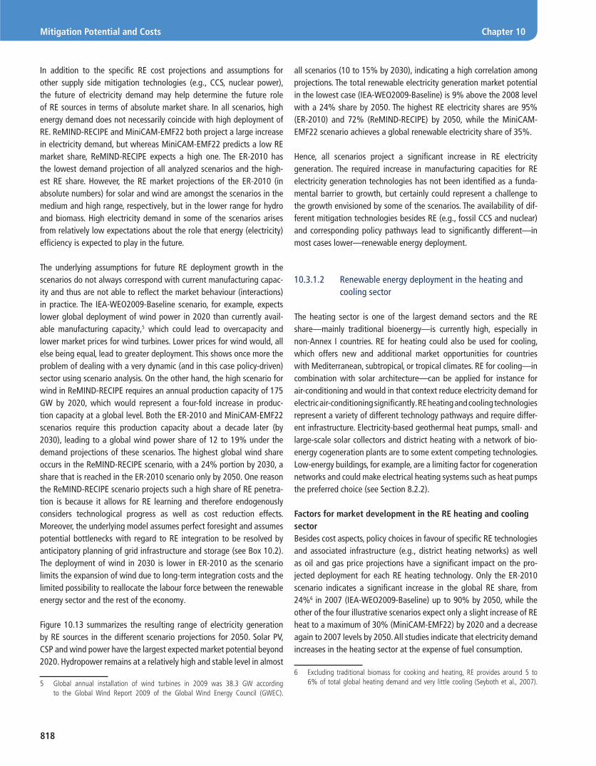
818


In addition to the specifi c RE cost projections and assumptions for other supply side mitigation technologies (e.g., CCS, nuclear power), the future of electricity demand may help determine the future role of RE sources in terms of absolute market share. In all scenarios, high energy demand does not necessarily coincide with high deployment of RE. ReMIND-RECIPE and MiniCAM-EMF22 both project a large increase in electricity demand, but whereas MiniCAM-EMF22 predicts a low RE market share, ReMIND-RECIPE expects a high one. The ER-2010 has the lowest demand projection of all analyzed scenarios and the high-est RE share. However, the RE market projections of the ER-2010 (in absolute numbers) for solar and wind are amongst the scenarios in the medium and high range, respectively, but in the lower range for hydro and biomass. High electricity demand in some of the scenarios arises from relatively low expectations about the role that energy (electricity) effi ciency is expected to play in the future.

The underlying assumptions for future RE deployment growth in the scenarios do not always correspond with current manufacturing capac-ity and thus are not able to refl ect the market behaviour (interactions) in practice. The IEA-WEO2009-Baseline scenario, for example, expects lower global deployment of wind power in 2020 than currently avail-able manufacturing capacity,5 which could lead to overcapacity and lower market prices for wind turbines. Lower prices for wind would, all else being equal, lead to greater deployment. This shows once more the problem of dealing with a very dynamic (and in this case policy-driven) sector using scenario analysis. On the other hand, the high scenario for wind in ReMIND-RECIPE requires an annual production capacity of 175 GW by 2020, which would represent a four-fold increase in produc-tion capacity at a global level. Both the ER-2010 and MiniCAM-EMF22 scenarios require this production capacity about a decade later (by 2030), leading to a global wind power share of 12 to 19% under the demand projections of these scenarios. The highest global wind share occurs in the ReMIND-RECIPE scenario, with a 24% portion by 2030, a share that is reached in the ER-2010 scenario only by 2050. One reason the ReMIND-RECIPE scenario projects such a high share of RE penetra-tion is because it allows for RE learning and therefore endogenously considers technological progress as well as cost reduction effects. Moreover, the underlying model assumes perfect foresight and assumes potential bottlenecks with regard to RE integration to be resolved by anticipatory planning of grid infrastructure and storage (see Box 10.2). The deployment of wind in 2030 is lower in ER-2010 as the scenario limits the expansion of wind due to long-term integration costs and the limited possibility to reallocate the labour force between the renewable energy sector and the rest of the economy.

Figure 10.13 summarizes the resulting range of electricity generation by RE sources in the different scenario projections for 2050. Solar PV, CSP and wind power have the largest expected market potential beyond 2020. Hydropower remains at a relatively high and stable level in almost

5 Global annual installation of wind turbines in 2009 was 38.3 GW according to the Global Wind Report 2009 of the Global Wind Energy Council (GWEC).

all scenarios (10 to 15% by 2030), indicating a high correlation among projections. The total renewable electricity generation market potential in the lowest case (IEA-WEO2009-Baseline) is 9% above the 2008 level with a 24% share by 2050. The highest RE electricity shares are 95% (ER-2010) and 72% (ReMIND-RECIPE) by 2050, while the MiniCAM-EMF22 scenario achieves a global renewable electricity share of 35%.

Hence, all scenarios project a signifi cant increase in RE electricity generation. The required increase in manufacturing capacities for RE electricity generation technologies has not been identifi ed as a funda-mental barrier to growth, but certainly could represent a challenge to the growth envisioned by some of the scenarios. The availability of dif-ferent mitigation technologies besides RE (e.g., fossil CCS and nuclear) and corresponding policy pathways lead to signifi cantly different—in most cases lower—renewable energy deployment.

10.3.1.2 Renewable energy deployment in the heating and cooling sector

The heating sector is one of the largest demand sectors and the RE share—mainly traditional bioenergy—is currently high, especially in non-Annex I countries. RE for heating could also be used for cooling, which offers new and additional market opportunities for countries with Mediterranean, subtropical, or tropical climates. RE for cooling—in combination with solar architecture—can be applied for instance for air-conditioning and would in that context reduce electricity demand for electric air-conditioning signifi cantly. RE heating and cooling technologies represent a variety of different technology pathways and require differ-ent infrastructure. Electricity-based geothermal heat pumps, small- and large-scale solar collectors and district heating with a network of bio-energy cogeneration plants are to some extent competing technologies. Low-energy buildings, for example, are a limiting factor for cogeneration networks and could make electrical heating systems such as heat pumps the preferred choice (see Section 8.2.2).

Factors for market development in the RE heating and cooling sectorBesides cost aspects, policy choices in favour of specifi c RE technologies and associated infrastructure (e.g., district heating networks) as well as oil and gas price projections have a signifi cant impact on the pro-jected deployment for each RE heating technology. Only the ER-2010 scenario indicates a signifi cant increase in the global RE share, from 24%6 in 2007 (IEA-WEO2009-Baseline) up to 90% by 2050, while the other of the four illustrative scenarios expect only a slight increase of RE heat to a maximum of 30% (MiniCAM-EMF22) by 2020 and a decrease again to 2007 levels by 2050. All studies indicate that electricity demand increases in the heating sector at the expense of fuel consumption.

6 Excluding traditional biomass for cooking and heating, RE provides around 5 to 6% of total global heating demand and very little cooling (Seyboth et al., 2007).

819


[TW

h/yr

]

[EJ/

yr]

PV CSP Wind Energy (On + Offshore)

GeothermalEnergy

Bioenergy Ocean Energy Hydropower

0

21,000

20,000

19,000

18.000

17,000

16,000

15,000

14,000

13,000

12,000

11,000

10,000

9,000

8,000

7,000

6,000

5,000

4,000

3,000

2,000

1,000

2020

2030

2050

2020

2030

2050

2020

2030

2050

2050

2020

2030

2050

2020

2030

2050

2020

2030

2050

2020

2030

Global Renewable Power Generation Development by Technology

54

72

36

18

IEA-WEO2009-Baseline

ReMIND-RECIPE

MiniCAM-EMF22

ER-2010

10% of Global Power Supply - ER Projection by 2050

10% of Global Power Supply - ReMIND Projection by 2050

10% of Global Power Supply - IEA-WEO Projection by 2050

Figure 10.13 | Global RE electricity generation (development projections by technology and shares of global power generation for the four illustrative scenarios for comparison). The total renewable power generation by 2050 is 11,159 TWh/yr (IEA-WEO2009-Baseline), 63,384 TWh/yr (ReMIND-RECIPE), 21,660 TWh/yr (MiniCAM-EMF22) and 41,500 TWh/yr (ER-2010) respectively. Sources: IEA-WEO2009-Baseline (IEA, 2009; Teske et al., 2010), ReMIND-RECIPE (Luderer et al., 2009), MiniCAM-EMF22 (Calvin et al., 2009), ER-2010 (Teske et al., 2010).

Annual market potential for RE heating and cooling The RE heating sector shows for the various technologies much lower growth rate projections than outlined for the electricity sector. The highest growth rates are expected for solar heating—especially solar collectors for water heating and space heating—followed by geo-thermal heating. Geothermal heating includes heat pumps, while geothermal cogeneration plants are presented in Section 10.3.2.1 under RE electricity generation.

In the ER-2010 scenario, solar heating systems show a signifi cant increase with market growth rates of above 35% until 2020 and a mini-mum of 10% afterwards up to the end of the projection in the year 2050 (see Section 3.4).

A shift from the traditional and sometimes unsustainable use of bioenergy for heating towards modern and more sustainable uses

of bioenergy heating such as wood pellet ovens or biogas burn-ers are assumed in all scenarios. The more effi cient use of biomass would increase the share of biomass heating without the necessity to increase the overall demand for biomass. However, only one of the analyzed scenarios provides information about the specifi c breakdown of traditional versus modern biomass use. Therefore, it is not possible to estimate the real annual market development of the different bio-energy heating systems.

The market potential at both domestic and industrial scales for RE heat-ing technologies such as solar collectors, geothermal heat pumps or pellet heating systems overlaps with the market potential analysis of the RE power sector. While the solar collector market is independent from the electricity sector, biomass cogeneration provides electricity as well as heat. Geothermal heat pumps use electricity for their operation and therefore increase the demand for electricity. RE heating and cooling

820


is more dispersed than RE electricity generation, which, together with lack of metering, is why statistical data are poor and further research is needed. Based on the energy parameters of the four scenarios ana-lyzed, the required annual market volume has been calculated in order to identify the needed manufacturing capacities and how they relate to current capacities. Table 10.5 provides an overview of the projected annual market volumes.

Manufacturing capacities for all RE heating and cooling technologies must be expanded signifi cantly in order to realize the projected RE heat production in all scenarios. The annual market volume for solar collec-tors is projected to triple from less than 35 PJ/yr in 2020 to 100 PJ/yr in 2030 in the IEA-WEO2009-Baseline case and up to 1,162 PJ/yr in the ER-2010 case. Due to the diverse technology options for bio- and geo-thermal energy heating systems and the low level of information in all analyzed scenarios, it is not possible to provide here a full set of specifi c market size data by technology.

The total share of RE heating systems in all scenarios by 2050 signifi cantly varies, from a market share of around 23% (IEA-WEO2009-Baseline, ReMIND-RECIPE and MiniCAM-EMF22) to 91% (ER-2010). The resulting shares for RE technologies for heating and cooling are signifi cantly driven by the scenario assumptions (including assumptions about infrastructure changes such as the expansion of district heating networks, as well as improvements in building effi ciency and industrial processes). The large share of RE heating systems in ER-2010 depends, for instance, on the assumption that district heating systems for the dis-tribution of solar-, geothermal- and bioenergy-generated heat would be available and competitive after 2020 (see Table 10.5).

10.3.1.3 Renewable energy deployment in the transport sector

The use of RE in the transport sector in all analyzed studies was limited to liquid biofuels, biomethane from biogas and RE-based electric vehi-cles for private use or public transport. Most of the scenario literature does not take into account new technologies such as second-generation sails for ships. Additionally, different reporting and categorization within the underlying scenario models do not support a stringent comparison of scenario results. However, even this comparison shows the substan-tial infl uence of driving forces (e.g., GHG stabilization levels) on the resulting RE share, which differs between scenarios by up to an order of magnitude (see Table 10.6).

10.3.1.4 Global renewable energy primary energy contribution

Figure 10.14 provides an overview of the projected primary energy pro-duction (using the direct equivalent methodology, see Section 1.1.8) by source for the four selected scenarios for 2020, 2030 and 2050, and compares the numbers with different projected global primary energy demands. Bioenergy has the highest market share, on average, across all of the scenarios, followed by solar energy, though scenario-specifi c

results vary. This is largely driven by the fact that bioenergy (see Chapter 2) can be used across all sectors (electricity, heating and cooling as well as transport) in combination with the selected primary energy account-ing methodology. As the available land for bioenergy is limited and competition with nature conservation issues as well as food and materi-als production is crucial, the sectoral use for the available bioenergy signifi cantly depends on scenario assumptions and underlying priorities (see Sections 2.2, 2.5 and 9.3.4). Solar energy can be used in direct form for heating and cooling and electricity generation (and indirectly via electricity for transport purposes), but solar technology starts from a relatively low level. The relatively lower average primary energy share for wind and hydropower may in part be due to their exclusive use in the electricity sector, though some scenarios show substantial contributions from wind in particular.

The total RE share in the primary energy mix by 2050 has a substan-tial variation across all four scenarios. With 15% by 2050—compared to 12.9% in 2008—the IEA-WEO2009-Baseline projects the lowest primary RE share, while ER-2010 reaches 77%, the MiniCAM-EMF22 achieves 31% and ReMIND-RECIPE 48% of the worlds primary energy demand with RE. While it is not surprising that without constrain-ing GHG concentration levels, RE deployment rates are rather low (IEA-WEO2009-Baseline), it is worth mentioning that there is even a signifi cant difference (more than a factor of two with regard to the relative RE shares) between the mitigation-oriented scenarios. Once more, this is a result of many aspects; that is, technology-specifi c assumptions (e.g., costs) and model characteristics (e.g., inclusion of endogenous learning), assumptions about the availability of other mitigation technologies and the expected energy demand. The over-all total global RE deployment by 2050 in all analyzed scenarios represents less than 2% of the available technical RE potential (see Section 10.3.2.2). The wide range of RE shares is a function of dif-ferent assumptions about policy, technology costs, chosen mitigation technologies (e.g., availability of CCS) and future energy demand projections.

10.3.2 Regional breakdown – technical potential versus market deployment

This section focuses on the regional perspective and provides an over-view of the regional market penetration paths given in the four scenarios. A comparison with the technical potential per region for each technol-ogy indicates to what level the regional technical potentials will be exploited. Additionally, an in-depth cost curve analysis of three regions (China, India and Europe) provides deeper insights into the assumed cost development of renewable electricity generation.

10.3.2.1 Regional renewable energy supply curves

Regional energy supply cost curves can serve as ‘snapshots’ of the selected scenarios and are thus an alternative perspective on scenario

821


Tabl

e 10

.5| P

roje

cted

RE

heat

pro

duct

ion,

pos

sible

mar

ket s

hare

s, an

nual

gro

wth

rate

s an

d an

nual

mar

ket v

olum

es fo

r the

four

illu

stra

tive

scen

ario

s—ex

cludi

ng a

dditi

onal

nee

ds fo

r re-

pow

erin

g. “

N/A

”: d

ata

not a

vaila

ble.

Sou

rces

: IEA

-W

EO20

09-B

asel

ine

(IEA,

200

9; Te

ske

et a

l., 20

10),

ReM

IND-

RECI

PE (L

uder

er e

t al.,

2009

), M

iniC

AM-E

MF2

2 (C

alvi

n et

al.,

2009

), ER

- 201

0 (T

eske

et a

l., 20

10).

Ener

gy P

aram

eter

Mar

ket

Dev

elop

men

t

Gen

erat

ion

[EJ/

yr]

Perc

ent

of g

loba

l dem

and

base

d on

dem

and

proj

ecti

ons

of t

he s

cena

rios

(inc

l. CH

P)

[%]

Ann

ual M

arke

t gr

owth

[%

/yr]

Ann

ual M

arke

t Vol

ume

[PJ/

yr]

IEA

-WEO

2009

-

Base

line

ReM

IND

-

RECI

PE

Min

iCA

M-

EMF2

2ER

-201

0

IEA

-WEO

2009

-

Base

line

ReM

IND

-

RECI

PE

Min

iCA

M-

EMF2

2ER

-201

0

IEA

-WEO

2009

-

Base

line

ReM

IND

-

RECI

PE

Min

iCA

M-

EMF2

2ER

-201

0

IEA

-WEO

2009

-

Base

line

ReM

IND

-

RECI

PE

Min

iCA

M-

EMF2

2ER

-201

0

Tota

l pro

ject

ed h

eat

dem

and

by s

cena

rio:

2020

158

190

135

152

2030

174

198

145

156

2050

205

160

151

152

Sola

r

Sola

r The

rmal

202

00.

8N

/AN

/A6.

50.

5N

/AN

/A4.

510

N/A

N/A

3932

N/A

N/A

409

Sola

r The

rmal

203

01.

6N

/AN

/A15

.80.

9N

/AN

/A12

.28

N/A

N/A

1210

0N

/AN

/A11

62

Sola

r The

rmal

205

03.

1N

/AN

/A38

.71.

5N

/AN

/A33

.73

N/A

N/A

518

7N

/AN

/A15

68

Geo

ther

mal

hea

ting

2020

0.6

0.1

N/A

4.4

0.4

0.1

N/A

3.0

14-6

N/A

416

-1N

/A63

2030

0.9

0.2

N/A

9.3

0.5

0.1

N/A

7.0

47

N/A

1012

3N

/A14

9

2050

1.6

4.6

N/A

26.5

0.8

2.8

N/A

26.4

318

N/A

722

66N

/A28

3

Bioe

nerg

y he

atin

g

2020

36.2

40.8

40.4

41.7

23.0

21.5

30.0

27.6

not s

peci

fi cal

ly m

odel

led

2811

210

413

0

2030

38.2

39.8

39.0

45.4

22.0

20.1

27.0

29.7

678

698

686

811

2050

43.6

32.4

31.7

48.1

21.3

20.2

21.0

31.7

270

191

186

295

Tota

l ren

ewab

les

heat

ing

2020

37.7

40.9

40.4

52.6

23.9

21.6

20.0

35.0

1N

/AN

/A5

66N

/AN

/A60

1

2030

40.7

40.0

39.0

70.5

23.4

20.2

27.0

48.7

1N

/AN

/A4

791

N/A

N/A

2122

2050

48.4

37.0

31.7

113.

323

.623

.121

.090

.81

N/A

N/A

347

9N

/AN

/A21

46

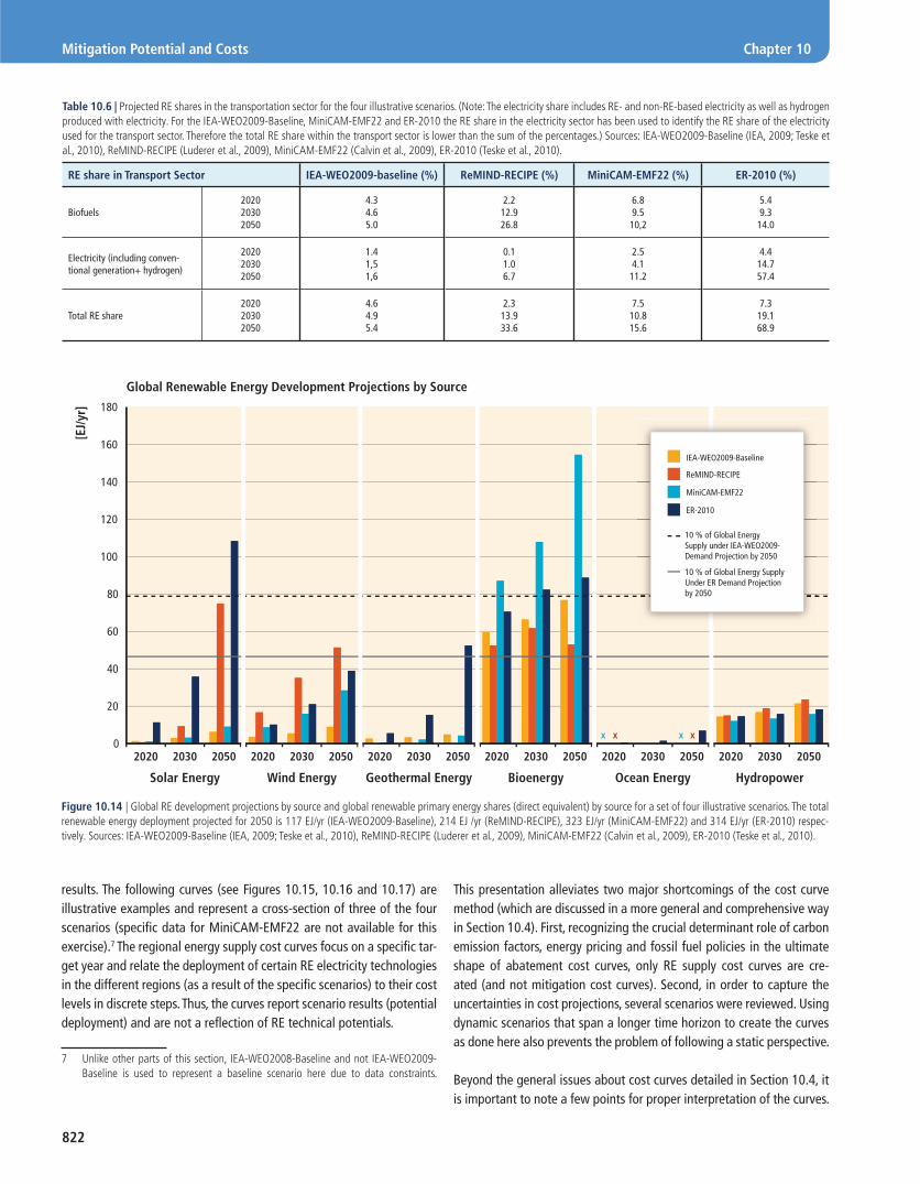
822


results. The following curves (see Figures 10.15, 10.16 and 10.17) are illustrative examples and represent a cross-section of three of the four scenarios (specifi c data for MiniCAM-EMF22 are not available for this exercise).7 The regional energy supply cost curves focus on a specifi c tar-get year and relate the deployment of certain RE electricity technologies in the different regions (as a result of the specifi c scenarios) to their cost levels in discrete steps. Thus, the curves report scenario results (potential deployment) and are not a refl ection of RE technical potentials.

7 Unlike other parts of this section, IEA-WEO2008-Baseline and not IEA-WEO2009-Baseline is used to represent a baseline scenario here due to data constraints.

X X X X

[EJ/

yr]

Solar Energy Wind Energy Geothermal Energy Bioenergy Ocean Energy Hydropower

0

100

80

60

40

20

120

140

180

160

2020 2030 2050 2020 2030 2050 2020 2030 2050 2020 2030 2050 2020 2030 2050 2020 2030 2050

10 % of Global Energy Supply under IEA-WEO2009-Demand Projection by 2050

10 % of Global Energy Supply Under ER Demand Projection by 2050

Global Renewable Energy Development Projections by Source


ReMIND-RECIPE

MiniCAM-EMF22

ER-2010

Figure 10.14 | Global RE development projections by source and global renewable primary energy shares (direct equivalent) by source for a set of four illustrative scenarios. The total renewable energy deployment projected for 2050 is 117 EJ/yr (IEA-WEO2009-Baseline), 214 EJ /yr (ReMIND-RECIPE), 323 EJ/yr (MiniCAM-EMF22) and 314 EJ/yr (ER-2010) respec-tively. Sources: IEA-WEO2009-Baseline (IEA, 2009; Teske et al., 2010), ReMIND-RECIPE (Luderer et al., 2009), MiniCAM-EMF22 (Calvin et al., 2009), ER-2010 (Teske et al., 2010).

This presentation alleviates two major shortcomings of the cost curve method (which are discussed in a more general and comprehensive way in Section 10.4). First, recognizing the crucial determinant role of carbon emission factors, energy pricing and fossil fuel policies in the ultimate shape of abatement cost curves, only RE supply cost curves are cre-ated (and not mitigation cost curves). Second, in order to capture the uncertainties in cost projections, several scenarios were reviewed. Using dynamic scenarios that span a longer time horizon to create the curves as done here also prevents the problem of following a static perspective.

Beyond the general issues about cost curves detailed in Section 10.4, it is important to note a few points for proper interpretation of the curves.

Table 10.6 | Projected RE shares in the transportation sector for the four illustrative scenarios. (Note: The electricity share includes RE- and non-RE-based electricity as well as hydrogen produced with electricity. For the IEA-WEO2009-Baseline, MiniCAM-EMF22 and ER-2010 the RE share in the electricity sector has been used to identify the RE share of the electricity used for the transport sector. Therefore the total RE share within the transport sector is lower than the sum of the percentages.) Sources: IEA-WEO2009-Baseline (IEA, 2009; Teske et al., 2010), ReMIND-RECIPE (Luderer et al., 2009), MiniCAM-EMF22 (Calvin et al., 2009), ER-2010 (Teske et al., 2010).

RE share in Transport Sector IEA-WEO2009-baseline (%) ReMIND-RECIPE (%) MiniCAM-EMF22 (%) ER-2010 (%)

Biofuels202020302050

4.34.65.0

2.212.926.8

6.89.510,2

5.49.314.0

Electricity (including conven-tional generation+ hydrogen)

202020302050

1.41,51,6

0.11.06.7

2.54.111.2

4.414.757.4

Total RE share202020302050

4.64.95.4

2.313.933.6

7.510.815.6

7.319.168.9

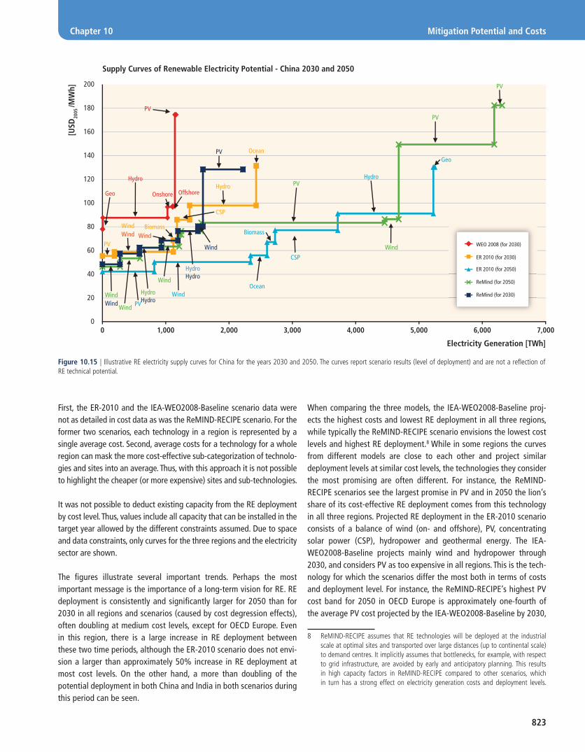
823


When comparing the three models, the IEA-WEO2008-Baseline proj-ects the highest costs and lowest RE deployment in all three regions, while typically the ReMIND-RECIPE scenario envisions the lowest cost levels and highest RE deployment.8 While in some regions the curves from different models are close to each other and project similar deployment levels at similar cost levels, the technologies they consider the most promising are often different. For instance, the ReMIND-RECIPE scenarios see the largest promise in PV and in 2050 the lion’s share of its cost-effective RE deployment comes from this technology in all three regions. Projected RE deployment in the ER-2010 scenario consists of a balance of wind (on- and offshore), PV, concentrating solar power (CSP), hydropower and geothermal energy. The IEA-WEO2008-Baseline projects mainly wind and hydropower through 2030, and considers PV as too expensive in all regions. This is the tech-nology for which the scenarios differ the most both in terms of costs and deployment level. For instance, the ReMIND-RECIPE’s highest PV cost band for 2050 in OECD Europe is approximately one-fourth of the average PV cost projected by the IEA-WEO2008-Baseline by 2030,

8 ReMIND-RECIPE assumes that RE technologies will be deployed at the industrial scale at optimal sites and transported over large distances (up to continental scale) to demand centres. It implicitly assumes that bottlenecks, for example, with respect to grid infrastructure, are avoided by early and anticipatory planning. This results in high capacity factors in ReMIND-RECIPE compared to other scenarios, which in turn has a strong effect on electricity generation costs and deployment levels.

Electricity Generation [TWh]

7,0006,0005,0004,0003,0002,0001,0000

[USD

2005

/MW

h]

20

0

40

60

80

100

120

140

160

180

200

PVPV

PV

PV

WindWind

WindWind

Wind

Wind

Wind

Wind

Wind

WindBiomass

Biomass

PV

PV

Ocean

Ocean

Hydro

CSP

CSP

Hydro Hydro

HydroHydro

HydroHydro

Onshore OffshoreGeo

Geo

Supply Curves of Renewable Electricity Potential - China 2030 and 2050

PV

ReMind (for 2050)

ER 2010 (for 2050)

ReMind (for 2030)

ER 2010 (for 2030)

WEO 2008 (for 2030)

Figure 10.15 | Illustrative RE electricity supply curves for China for the years 2030 and 2050. The curves report scenario results (level of deployment) and are not a refl ection of RE technical potential.

First, the ER-2010 and the IEA-WEO2008-Baseline scenario data were not as detailed in cost data as was the ReMIND-RECIPE scenario. For the former two scenarios, each technology in a region is represented by a single average cost. Second, average costs for a technology for a whole region can mask the more cost-effective sub-categorization of technolo-gies and sites into an average. Thus, with this approach it is not possible to highlight the cheaper (or more expensive) sites and sub-technologies.

It was not possible to deduct existing capacity from the RE deployment by cost level. Thus, values include all capacity that can be installed in the target year allowed by the different constraints assumed. Due to space and data constraints, only curves for the three regions and the electricity sector are shown.

The fi gures illustrate several important trends. Perhaps the most important message is the importance of a long-term vision for RE. RE deployment is consistently and signifi cantly larger for 2050 than for 2030 in all regions and scenarios (caused by cost degression effects), often doubling at medium cost levels, except for OECD Europe. Even in this region, there is a large increase in RE deployment between these two time periods, although the ER-2010 scenario does not envi-sion a larger than approximately 50% increase in RE deployment at most cost levels. On the other hand, a more than doubling of the potential deployment in both China and India in both scenarios during this period can be seen.

824


Figure 10.16 | Illustrative RE electricity supply curves for India for the years 2030 and 2050. The curves report scenario results (level of deployment) and are not a refl ection of RE technical potential.


3,0002,5002,0001,5001,0005000

[USD

2005

/MW

h]

20

0

40

60

80

100

120

140

160

180

200

Supply Curves of Renewable Electricity Potential - India 2030 and 2050

ReMind (for 2050)

ER 2010 (for 2050)

ReMind (for 2030)

ER 2010 (for 2030)

WEO 2008 (for 2030)

PV

PV

PVPV Wind

Wind

Wind

WindWind PV

PV

PV

PV

PVPV

Wind

Wind

Wind

Wind

Biomass

Biomass

CSP

CSP

Hydro

Hydro

Hydro

Hydro

Hydro

Onshore

Ocean

Ocean

Offshore

GeoGeo


4,0003,5003,0002,5002,0001,5001,0005000

[USD

2005

/MW

h]

0

50

100

150

200

250

300

Supply Curves of Renewable Electricity Potential - OECD Europe 2030 and 2050

ReMind (for 2050)

ER 2010 (for 2050)

ReMind (for 2030)

ER 2010 (for 2030)

WEO 2008 (for 2030)PV

PV

PV

PV

PVPV

PV

PV

WindWind

Wind

WindWind

WindWind

Wind

Biomass

Biomass

Ocean OceanWind

PV

CSP CSPCSP

Hydro

Hydro

Hydro

Hydro

Hydro

Hydro

Hydro

Onshore

Ocean

Offshore

Geo

Geo

Geo

Figure 10.17 | Illustrative RE electricity supply curves for OECD Europe for the years 2030 and 2050. The curves report scenario results (level of deployment) and are not a refl ection of RE technical potential.

825


Figure 10.18 | Regional breakdown of possible energy demand and RE potential deployment for the selected set of four scenarios in 2050 (direct equivalent). Sources: IEA-WEO2009-Baseline (IEA, 2009; Teske et al., 2010), ReMIND-RECIPE (Luderer et al., 2009), MiniCAM-EMF22 (Calvin et al., 2009), ER-2010 (Teske et al., 2010). For comparison, total primary energy demand in 2007 is given (IEA, 2009).

XXXXX

[EJ/

yr]

0

20

40

60

80

100

120

140

160

180

200

220

240

260

280

300

320

340

OECDEurope

OECDNorth America

OECDPacific

Latin America

Trans. Economies

DevelopingAsia

Africa Middle East


ReMIND-RECIPE

MiniCAM-EMF22

ER-2010

Regional Primary Energy Demand in 2007

Total Renewable EnergyDeployment Within Scenario

X

Projected Renewable Energy Deployment in Different Scenarios by Region for 2050

No Numbers Aggregatedfor this Region

and even the highest cost band in 2030 is half the average PV cost projected by that same study.

The different scenarios see different roles and costs for CSP. ReMIND-RECIPE considers a generic solar technology parameterized based on PV, and thus this technology was not specifi cally modelled in this scenario. The ER-2010 scenarios see a larger role for CSP than for PV in both China and India in the longer term, albeit at a higher cost. Neither of the models attributes a major deployment of geothermal energy, but they see its costs very differently. The costs of this electricity generation source in the IEA-WEO2008-Baseline is approximately half of that in the ER-2010 scenarios for the same target year (2030), and even in 2050 the ER-2010 cost projections are signifi cantly higher for this technology than in the IEA-WEO2008-Baseline scenario in 2030—although the deployment levels at this cost are several times higher than projected by the other scenarios, making a noticeable contribution to the total deployment in 2050 in India and OECD Europe from among the examined regions. The ReMIND-RECIPE scenarios do not consider geothermal power.

With regard to the quality of electricity supply, it is also important to keep in mind that the presented supply curves do not distinguish between highly variable, and sometimes unpredictable, energy sources and dispatchable energy sources. In this context, a cost premium due to

a higher reliability level that might be needed is also not considered as additional backup costs for highly variable RE sources.

10.3.2.2 Primary energy by region, technology and sector

This section provides an overview of the potential deployment paths given in the four scenarios versus the technical potential per region. For each technology, deployment shares indicate to what level the regional technical potential has been exploited. Figure 10.19 compares the resulting primary energy contribution of RE in relation to the tech-nical potential by region and technology for the four scenarios, while Figure 10.18 gives an overview for all scenarios, but for RE as a whole by region, compared to the demand projections by 2050 and the current regional primary energy demand.

The maximum deployment share out of the overall technical potential for RE in 2050 was found for India with a total of 22.1% (ER-2010), followed by China with a total of 17.7% (ER-2010) and OECD Europe 15.3% (ER-2010). Two regions had deployment rates of about 5 to 7% of the regional available technical RE potential by 2050: 6.9% in developing Asia (MiniCAM-EMF22) and 5.5% for OECD North America (ER-2010). The remaining fi ve regions used less than 4.5% of the

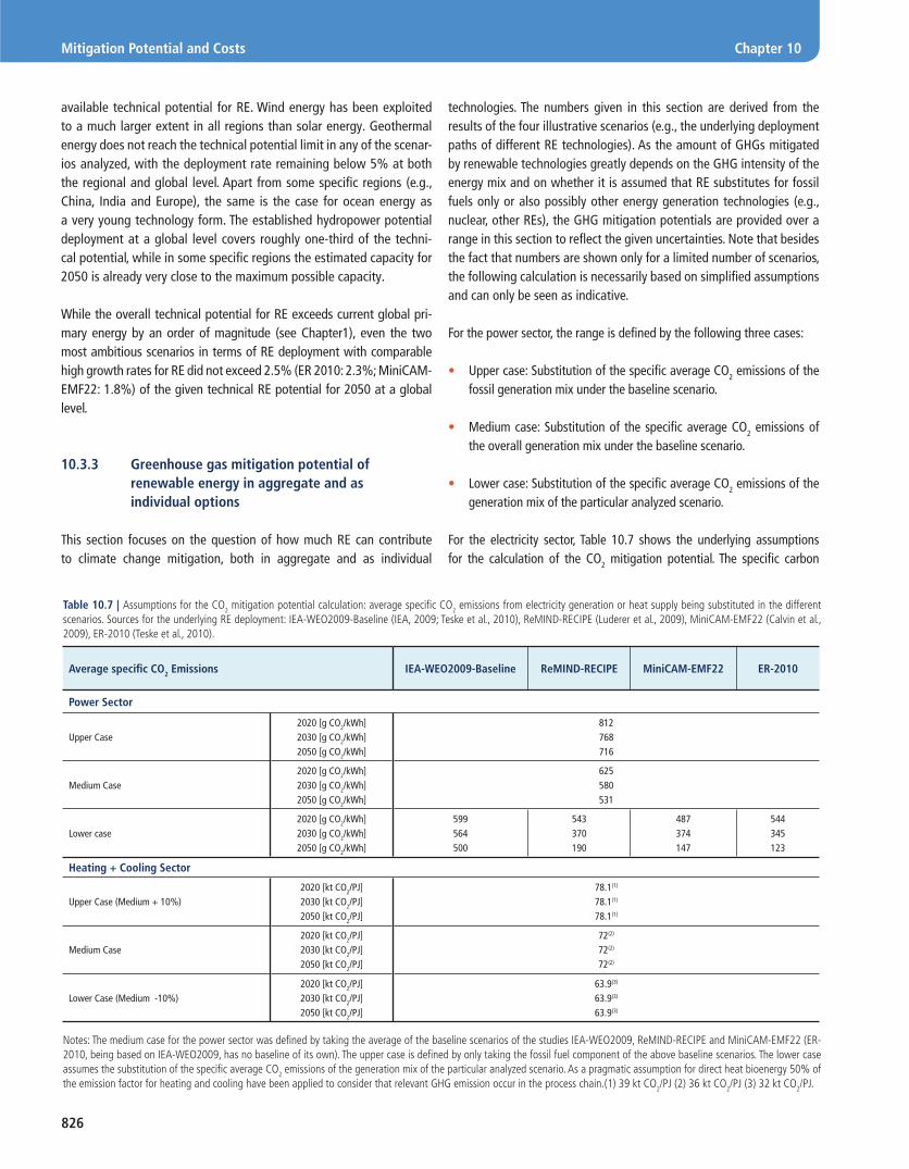
826


available technical potential for RE. Wind energy has been exploited to a much larger extent in all regions than solar energy. Geothermal energy does not reach the technical potential limit in any of the scenar-ios analyzed, with the deployment rate remaining below 5% at both the regional and global level. Apart from some specifi c regions (e.g., China, India and Europe), the same is the case for ocean energy as a very young technology form. The established hydropower potential deployment at a global level covers roughly one-third of the techni-cal potential, while in some specifi c regions the estimated capacity for 2050 is already very close to the maximum possible capacity.

While the overall technical potential for RE exceeds current global pri-mary energy by an order of magnitude (see Chapter1), even the two most ambitious scenarios in terms of RE deployment with comparable high growth rates for RE did not exceed 2.5% (ER 2010: 2.3%; MiniCAM-EMF22: 1.8%) of the given technical RE potential for 2050 at a global level.

10.3.3 Greenhouse gas mitigation potential of renewable energy in aggregate and as

individual options

This section focuses on the question of how much RE can contribute to climate change mitigation, both in aggregate and as individual

technologies. The numbers given in this section are derived from the results of the four illustrative scenarios (e.g., the underlying deployment paths of different RE technologies). As the amount of GHGs mitigated by renewable technologies greatly depends on the GHG intensity of the energy mix and on whether it is assumed that RE substitutes for fossil fuels only or also possibly other energy generation technologies (e.g., nuclear, other REs), the GHG mitigation potentials are provided over a range in this section to refl ect the given uncertainties. Note that besides the fact that numbers are shown only for a limited number of scenarios, the following calculation is necessarily based on simplifi ed assumptions and can only be seen as indicative.

For the power sector, the range is defi ned by the following three cases:

• Upper case: Substitution of the specifi c average CO2 emissions of the fossil generation mix under the baseline scenario.

• Medium case: Substitution of the specifi c average CO2 emissions of the overall generation mix under the baseline scenario.

• Lower case: Substitution of the specifi c average CO2 emissions of the generation mix of the particular analyzed scenario.

For the electricity sector, Table 10.7 shows the underlying assumptions for the calculation of the CO2 mitigation potential. The specifi c carbon

Table 10.7 | Assumptions for the CO2 mitigation potential calculation: average specifi c CO2 emissions from electricity generation or heat supply being substituted in the different scenarios. Sources for the underlying RE deployment: IEA-WEO2009-Baseline (IEA, 2009; Teske et al., 2010), ReMIND-RECIPE (Luderer et al., 2009), MiniCAM-EMF22 (Calvin et al., 2009), ER-2010 (Teske et al., 2010).

Average specifi c CO2 Emissions IEA-WEO2009-Baseline ReMIND-RECIPE MiniCAM-EMF22 ER-2010

Power Sector

Upper Case2020 [g CO2/kWh]2030 [g CO2/kWh]2050 [g CO2/kWh]

812768716

Medium Case 2020 [g CO2/kWh]2030 [g CO2/kWh]2050 [g CO2/kWh]

625580531

Lower case2020 [g CO2/kWh]2030 [g CO2/kWh]2050 [g CO2/kWh]

599 564 500

543 370 190

487 374 147

544345123

Heating + Cooling Sector

Upper Case (Medium + 10%) 2020 [kt CO2/PJ]2030 [kt CO2/PJ]2050 [kt CO2/PJ]

78.1(1)

78.1(1)

78.1(1)

Medium Case 2020 [kt CO2/PJ]2030 [kt CO2/PJ]2050 [kt CO2/PJ]

72(2)

72(2)

72(2)

Lower Case (Medium -10%)2020 [kt CO2/PJ]2030 [kt CO2/PJ]2050 [kt CO2/PJ]

63.9(3)

63.9(3)

63.9(3)

Notes: The medium case for the power sector was defi ned by taking the average of the baseline scenarios of the studies IEA-WEO2009, ReMIND-RECIPE and MiniCAM-EMF22 (ER-2010, being based on IEA-WEO2009, has no baseline of its own). The upper case is defi ned by only taking the fossil fuel component of the above baseline scenarios. The lower case assumes the substitution of the specifi c average CO2 emissions of the generation mix of the particular analyzed scenario. As a pragmatic assumption for direct heat bioenergy 50% of the emission factor for heating and cooling have been applied to consider that relevant GHG emission occur in the process chain.(1) 39 kt CO2/PJ (2) 36 kt CO2/PJ (3) 32 kt CO2/PJ.

827


Rang

e gr

aphs

: Lev

el o

f RE

Depl

oym

ent

in 2

050

by S

cena

rio a

nd R

enew

able

En

ergy

, in

EJ/y

r:

IEA-

WEO

2009

-Bas

elin

e

ReM

IND-

RECI

PE

Min

iCAM

-EM

F22

ER-2

010

Rang

e

050100

150

200

250

300

350

0-2.

52.

6-5.

05.

1-7.

57.

6-10

10-1

2.5

12.6

-15

15.1

-17.

517

.6-2

020

.1-2

2.5

22.6

-25

25-5

0O

ver 5

0

Direct Solar

Wind

Geothermal

Hydropower

Ocean

Bioenergy

Total

Wor

ld -

EJ/y

r

Tota

l Tec

hnic

al R

E Po

tent

ial

in E

J/yr

for

2050

by

Rene

wab

le E

nerg

y So

urce

:

Sola

r

Win

d

Geo

ther

mal

Hydr

o

Oce

an

Bio

ener

gy

X EJ

/yr

Tech

nica

l RE

Pote

ntia

l Can

Sup

ply

the

2007

Pri

mar

y En

ergy

Dem

and

by a

Fac

tor

of:

RE p

oten

tial a

naly

sis:

Tech

nica

l RE

pote

ntia

ls re

port

ed h

ere

repr

esen

t tot

al w

orld

wid

e an

d re

gion

al p

oten

tials

bas

ed o

n a

revi

ew o

f st

udie

s pu

blis

hed

befo

re 2

009

by K

rew

itt e

t al.

(200

9). T

hey

do n

ot d

educ

t any

pot

entia

l tha

t is

alre

ady

bein

g ut

ilize

d fo

r ene

rgy

prod

uctio

n. D

ue to

met

hodo

logi

cal d

iffer

ence

s an

d ac

coun

ting

met

hods

am

ong

stud

ies,

stric

t com

para

bilit

y of

thes

e es

timat

es a

cros

s te

chno

logi

es a

nd re

gion

s, as

wel

l as

to p

rimar

y en

ergy

dem

and,

is n

ot p

ossi

ble.

Tech

nica

l RE

pote

ntia

l ana

lyse

s pu

blis

hed

afte

r 200

9 sh

ow h

ighe

r res

ults

in s

ome

case

s bu

t are

not

incl

uded

in th

is fi

gure

. How

ever

, som

e RE

tech

nolo

gies

may

com

pete

for l

and

whi

ch

coul

d lo

wer

the

over

all R

E po

tent

ial.

Scen

ario

dat

a: IE

A W

EO 2

009

Refe

renc

e Sc

enar

io (I

nter

natio

nal E

nerg

y Ag

ency

(IEA

), 20

09; T

eske

et a

l., 2

010)

, ReM

IND-

RECI

PE 4

50pp

mSt

abili

zatio

n Sc

enar

io (L

uder

er e

t al.,

200

9), M

iniC

AM E

MF2

2 1s

t-be

st 2

.6 W

/2 O

vers

hoot

Sce

nario

(Cal

vin

et a

l., 2

009)

, Adv

ance

d En

ergy

[R]e

volu

tion

2010

(Tes

ke e

t al.,

201

0)

193

EJ/y

r

193

EJ/y

r

306

EJ/y

r

571

EJ/y

r

11,9

41 E

J/yr

1,33

5 EJ

/yr

5,36

0 EJ

/yr

864

EJ/y

r

761

EJ/y

r

1,91

1 EJ

/yr

464

EJ/y

r

828


OEC

D E

urop

e - E

J/yr

05101520253035

Direct Solar

Wind

Geothermal

Hydropower

Ocean

Bioenergy

Total

n

l

r

Dev

elop

ing

Asi

a - E

J/yr

0306090120

150

Direct Solar

Wind

Geothermal

Hydropower

Ocean

Bioenergy

Total

r

d

al

r

an

Tran

siti

on E

cono

mie

s - E

J/yr

0510152025

Direct Solar

Wind

Geothermal

Hydropower

Ocean

Bioenergy

Total

ar

d

al

n

OEC

D N

orth

Am

eric

a - E

J/yr

0102030405060

Direct Solar

Wind

Geothermal

Hydropower

Ocean

Bioenergy

Total

r

l

an

Lati

n A

mer

ica

- EJ/

yr

0510152025

Direct Solar

Wind

Geothermal

Hydropower

Ocean

Bioenergy

Total

an

al

d

r

OEC

D P

acifi

c - E

J/yr

05101520

Direct Solar

Wind

Geothermal

Hydropower

Ocean

Bioenergy

Total

n

l

r

Afr

ica

- EJ/

yr

051015202530

Direct Solar

Wind

Geothermal

Hydropower

Ocean

Bioenergy

Total

an

al

d

r

Mid

dle

East

- EJ

/yr

05101520

Direct Solar

Wind

Geothermal

Hydropower

Ocean

Bioenergy

Total

y

an

er

al

d

r

829


X X

10% Global CO2 Emission (Base 2008)

33% of Global CO2 Emission (Base 2008)

2030: IEA-WEO2009-Baseline

2050: IEA-WEO2009-Baseline

2030: ReMIND-RECIPE

2050: ReMIND-RECIPE

2030: MiniCAM-EMF22

2050: MiniCAM-EMF22

2030: ER-2010

2050: ER-2010

Annual Global CO2 Savings from RE by Technology in Four Deployment Scenarios for 2030 and 2050

[Gt

CO2 /y

r]

Solar Energy Wind Energy Geothermal Energy Bioenergy Ocean Energy Hydropower0

8

6

4

2

10

12

14

16

Figure 10.20 | Expected range of annual global CO2 savings from RE for the four illustrative scenarios for 2030 and 2050. Biofuels for transport are excluded, and biomass used for direct heating only accounts for half the CO2 savings due to imbedded GHG emissions from bioenergy. The presented range marks the high uncertainties regarding the substituted energy source: While the upper limit assumes full substitution of high-carbon fossil fuels, the lower limit considers specifi c CO2 emissions of the analyzed scenario itself. Sources: IEA-WEO2009-Baseline (IEA, 2009; Teske et al., 2010), ReMIND-RECIPE (Luderer et al., 2009), MiniCAM-EMF22 (Calvin et al., 2009), ER-2010 (Teske et al., 2010).For comparison, global CO2 emissions in 2008 are given (IEA 2010d).

Figure 10.19 | (Preceding pages) Overview of the relation between the primary energy contribution of RE (direct equivalent) and the corresponding technical potential for different technologies and regions for 2050 for the selected set of four scenarios. Due to differences in regional aggregation not all models provide data for all regions.

Note: Data for technical potential presented in Chapters 2 through 7 may disagree with the fi gures in Krewitt et al. (2009) due to differences in assessed studies and the underlying methodologies (see also Chapter 1, in which Krewitt et al. (2009) worldwide RE technical potential estimates are compared to a range of values in the literature presented in Chapters 2 through 7).

emissions factor for the year 2050 ranges from 716 g CO2/kWh (199 g CO2

/kJ) (upper case) to between 123 and 190 g CO2 /kWh (34 to 53 g CO2 /kJ) (lower case) for the selected mitigation scenarios. As noted in the table, a range of emission factors was also assumed for RE used in heating and cooling applications. In contrast to electricity generation, no specifi c infor-mation for these applications was available from the different scenarios. Against that background for the calculation, a pragmatic approach was selected for the underlying emission factors starting with a substitution of oil for the medium case and considering an uncertainty range.

Biofuels and other RE options for transport are excluded in the calcu-lation due to limited data availability. To refl ect the embedded GHG emissions saved due to bioenergy used for direct heating, only half of the theoretical CO2 savings have been considered in the calculation. Given the high uncertainties and variability of embedded GHG emis-sions (see Chapter 2 for the discussion of indirect GHG emissions from the whole biomass process chain and Chapter 9 for a more general discussion on lifecycle assessment of different RE sources) this is neces-sarily once more a simplifying assumption.

Figure 10.20 shows the resulting annual CO2 reduction potential by RE source for all scenarios for 2030 and 2050. The black line at 2.9 Gt CO2 /yr identifi es 10% of the global energy-related CO2 emissions; the red line here indicates 33% of total energy-related CO2 emissions (base year for both lines is 2008).

The three mitigation scenarios of the illustrative scenarios show a wide range of possible RE contribution. While in all three, hydropower and wind energy play leading roles in 2030, in two of the scenarios (ReMIND-RECIPE, ER-2010) solar energy supersedes the other technologies by 2050. In contrast, as discussed earlier, due to the specifi c primary energy accounting approach the primary energy share ranking is led by bio-energy (see Section 10.3.1.4). This shows that the contributions (and effectiveness) of RE technologies vary by what perspective is taken (GHG mitigation or primary energy perspective). Further, the dependence of the resulting impacts on underlying assumptions is of great importance.

The resulting GHG reduction potential of all RE technologies heavily depends on the complex system behaviour determining the substituted

830


energy sources. Considering the limitations of the rough approximations applied here, in the four scenarios the corresponding annual CO2 reduc-tion potential in 2050 reaches from 4.2 Gt CO2 /yr (MiniCAM-EMF22 lower case) to 35.3 Gt CO2 /yr (ER-2010 upper case) (Figure 10.21). At the upper level, this is equal to approximately 80% of the energy-related CO2 emissions of the analyzed baseline scenario (IEA-WEO2009-Baseline) in the year 2050.

Cumulative CO2 reduction potentials from RE sources up to 2020, 2030 and 2050 (Figure 10.22) have been calculated on the basis of the annual average CO2 savings shown in Figure 10.21.9 Based on this, the analyzed scenarios would have a cumulative reduction potential (2010 to 2050) in the medium case approach of between 244 Gt CO2 (IEA-WEO2009-Baseline) under the baseline conditions, 297 Gt CO2 (MiniCAM-EMF22), 482 Gt CO2 (ER-2010) and 490 Gt CO2 (ReMIND-RECIPE scenario). The full range across all calculated cases and scenarios for the cumulative CO2 savings is between 218 Gt CO2 (IEA-WEO2009-Baseline) and 561 Gt CO2 (ReMIND-RECIPE), compared to about 1,530 Gt CO2 cumulative fos-sil and industrial CO2 emissions in the IEA-WEO2009-Baseline scenario during the same period.

9 For the integration, the time periods 2020 to 2030 and 2030 to 2050 were linearly interpolated.

Again, these numbers exclude CO2 savings from RE use in the transport sector (including biofuels and electric vehicles). The overall CO2 mitiga-tion potential can therefore be higher.

10.3.4 Comparison of the results of the in-depth scenario analysis and knowledge gaps

All in-depth scenarios analyzed here show an increase in RE sources across all sectors. However, the electricity sector is in the forefront of all sectors and here the most dynamic increase in RE capacity is projected. Hydropower is expected to play the dominant role in the RE electricity sector in the near term and on a global basis, but based largely on already-existing installed generation capacity. Wind is expected in all three mitigation scenarios to overtake hydropower in terms of global electricity supply by 2030. The results for all other technologies are far more diverse. Two scenarios see solar PV as an important player in the electricity sector after 2030, with a share of more than 10% by 2050, while the baseline scenario projects PV remaining at marginal levels. In all but the ER-2010 scenario, the foreseen role for geothermal energy remains low at levels

Figure 10.21 | Range of annual global CO2 savings from RE in total for a set of four illustrative scenarios for 2030 and 2050 (Note: biofuels for transport are excluded, and biomass used for direct heating only accounts for half the CO2 savings due to embedded GHG emissions from bioenergy). (The presented range marks the high uncertainties regarding the substituted energy source: while the upper limit assumes a full substitution of high-carbon fossil fuels, the lower limit considers specifi c CO2 emissions of the analyzed scenario itself.) Sources: IEA-WEO2009-Baseline (IEA, 2009; Teske et al., 2010), ReMIND-RECIPE (Luderer et al., 2009), MiniCAM-EMF22 (Calvin et al., 2009), ER-2010 (Teske et al., 2010).

Annual Global CO2 Savings from RE for Different Scenario-Based Deployment Paths for 2030 and 2050

[Gt

CO2 /y

r]

20502030205020302050203020502030IEA-WEO2009-Baseline ReMind-Recipe MiniCAM-EMF22 ER-2010

15

10

5

0

20

25

30

35

40

Total Global Energy RelatedCO2 Emissions in 2008

30% of Global Energy Related CO2 Emissions in 2008

831


Figure 10.22 | Expected range of global cumulative CO2 savings up to 2020, 2030 and 2050. The presented range marks the high uncertainties regarding the substituted conventional energy source: while the upper limit assumes a full substitution of high-carbon fossil fuels, the lower limit considers specifi c CO2 emissions of the analyzed scenario itself. Sources: IEA-WEO2009-Baseline (IEA, 2009; Teske et al., 2010), ReMIND-RECIPE (Luderer et al., 2009), MiniCAM-EMF22 (Calvin et al., 2009), ER-2010 (Teske et al., 2010).

Global Cumulative CO2 Savings for Different Scenario-Based RE Deployment Paths 2010 up to 2020, 2030 and 2050

[Gt

CO2]

IEA-WEO2009-Baseline ReMind-RECIPE MiniCam-EMF22 ER-2010

100

0

200

300

400

500

600

2020 2030 2050 2020 2030 2050 2020 2030 2050 2020 2030 2050

well below 5% of the global electricity supply. The scenario results for the heating and cooling sector include signifi cant uncertainties as the models use different accounting methods, for example, for geothermal heat pumps. In terms of primary energy share, bioenergy has the greatest share—especially in the heating sector. Wind and solar energy are projected to become important players by and after 2030.

As already stressed in the comprehensive scenario survey (see Section 10.2), there are many reasons why the investigated scenarios reach different results. Each of the in-depth scenarios follows a different strat-egy. Signifi cant differences in the demand projections and whether or not a shift towards more electricity within the transport and/or heat-ing sector are projected to have a signifi cant impact on the selected technologies and their deployment rates. Moreover, other mitigation technologies, such as CCS and/or nuclear, have a signifi cant impact on the resulting role of RE sources in a future energy mix. In practice, a high RE deployment can only be achieved if system-relevant policy decisions are made many years ahead of the intended market penetration. The assumptions of expanded energy infrastructure such as transmission grids (see Chapter 8) or district heating networks can change the RE deploy-ment of the scenario entirely. Even if the analyzed models do not include

grid modelling via system integration aspects, these issues are at least covered implicitly in the scenarios (integration restrictions).

Due to comparably long lifetime expectations, the energy system is relatively infl exible and investment decisions have long-lasting impacts. A high share of relatively infl exible ‘base load’ power plants—such as coal, lignite and nuclear power plants, for instance—will reduce the technical and economic ‘space’ of variable renewable electricity generation like solar photovoltaic and wind. Technology choices and preferences pre-determine the future RE deployment as well as the assumed RE cost developments and corresponding fossil fuel price projections. The over-all share of RE in primary energy demand within the three in-depth mitigation scenario ranges from 24% (MiniCAM-EMF22) to 39% (ER-2010) by 2030 and 31% (MiniCAM-EMF22) to 77% (ER-2010) by 2050. Lower RE shares are due to the availability of competing low-carbon tech-nologies such as CCS and nuclear, while scenarios not allowing access to these technologies expect higher RE shares, but not necessarily higher absolute numbers.

In addition to the comprehensive scenario survey in the previous section (see Section 10.2), the in-depth analyses of the four illustrative scenarios

832


could deliver further specifi c insights into the specifi c RE technology deployment and the corresponding driving forces. However, often data availability limits detailed investigations. Against that background the following knowledge gaps can be identifi ed:

• Lack of consistent RE technical potential estimates across the globe, and especially in developing countries (consistent eco-nomic potential estimates are an important input basis for the models).

• Modelling of the heating and transport sectors in most of the exist-ing models is less detailed than modelling of the electricity sector, although both sectors are substantially contribute to GHG emis-sions. More generally, there is a severe lack of data for the heating and transport sector especially on a sectoral or regional basis.

• New RE technologies, such as ocean energy, are not represented in most of the current energy scenarios.

• The reporting system, for example, for geothermal heat pumps, is very different in all scenarios and sometimes not transparent, which makes it diffi cult to compare the results.

• The interaction of the technology pathways with the effects on deployment costs (learning effects) are treated differently in the scenarios and underlying assumptions or implemented calculation rules are sometimes not very well reported.

• Simplifi ed calculations of the resulting CO2 mitigation potential of RE deployment can give an orientation, but are associated with severe shortcomings. Comparative model runs (with and without RE) are necessary to consider the energy system behaviour in an appropriate way.

10.4 Regional cost curves for mitigation with renewable energies

10.4.1 Introduction

Governments and decision makers face limited fi nancial and insti-tutional resources and capacities for mitigation, and therefore tools that assist them in strategizing how these limited resources are prioritized have become very popular. Among these tools are abate-ment cost curves—a tool that relates the mitigation potential of a mitigation option to its marginal cost. Recent years have seen a major interest among decision- and policymakers in abatement cost curves, witnessed by the proliferation in the number of such stud-ies and institutions/companies engaged in preparing such reports (e.g., Next Energy, 2004; Creyts et al., 2007; Dornburg et al., 2007; McKinsey&Company, 2007, 2008a, 2009b,c; IEA, 2008b). However,

while abatement curves are very practical and can provide important strategic overviews, it is pertinent to understand that their use for decision making has many limitations.

The aims of this section are to: (a) review the concept of abatement cost curves briefl y and appraise their strengths and shortcomings (Section 10.4.2); (b) review the existing literature on regional abatement cost curves as they pertain to mitigation using RE (Section 10.4.3); and (c) review the literature on (regional) RE technology resource supply cost curves (Section 10.4.4). The section thus covers supply curves of RE on the one hand, which evaluate the unit costs of energy generation and the possibilities of utilizing the technical potential depending on the technology deployed, and on the other hand carbon abatement cost curves, which describe the mitigation potentials and marginal costs of emission mitigation (usually per tonne of CO2eq.) through the deployment of renewable energy sources.

10.4.2 Cost curves: concept, strengths and limitations

10.4.2.1 The concept

The concepts of supply curves of carbon abatement, energy, or con-served energy all rest on the same foundation. They are curves consisting typically of discrete steps, each step relating the marginal cost of the abatement measure/energy generation technology or measure to con-serve energy to its potential; these steps are ranked according to their cost. Graphically, the steps start at the lowest cost on the left with the next highest cost added to the right and so on, making an upward slop-ing left-to-right marginal cost curve. As a result, a curve is obtained that can be interpreted similarly to the concept of supply curves in traditional economics.

Supply curves of conserved energy were fi rst introduced by Arthur Rosenfeld (see Meier et al., 1983) and became a popular concept in the 1980s (Stoft, 1995). The methodology has since been revised and upgraded, and the fi eld of its application extended to energy generation supply curves including RE cost curves; as well as carbon abatement from the 1990s (Rufo, 2003). One of the benefi ts of the method was that it provided a framework for comparing otherwise different options, such as the cost-effectiveness of different energy supply options compared to energy conservation options, and therefore was a practical tool for some decision-making approaches, such as integrated resource plan-ning. Although Stoft (1995) explains why the supply curves used in the studies by Meier et al. (1983) cannot be regarded as ‘true’ supply curves, including the fact that markets associated with the different types of options depicted in them, such as energy effi ciency and energy supply markets, differ in many aspects, he maintains that they are useful for their purpose.

Despite the widespread use of supply curves and their advantages discussed above, there are some inherent limitations to the method

833


that have attracted criticism from various authors that are important to review before reviewing the literature on them or presenting the regional cost curves.

10.4.2.2 Limitations of the supply curve method

The concept of abatement, energy and conservation supply curves has common and specifi c limitations. Much of the criticism in the early and some later literature focuses on the notion of options with negative costs. For instance, IEA (2008b) raises an objection based on the perfect market theory from neoclassical economics, arguing that it is not possible to have negative cost options as under perfect market conditions someone must have realized those options com-plying with rational economic behaviour. The existence of untapped ‘profi table’ (i.e., negative cost) opportunities represents a realm of debates ongoing for decades between different schools of thought (e.g., see Carlsmith et al., 1990; Sutherland, 1991; Koomey et al. 1998; Gumerman et al., 2001). Those accepting negative cost opportuni-ties argue, among other things, that certain barriers prevent those investments from taking place on a purely market basis, but policy interventions can remove these barriers and unlock these profi table opportunities. Therefore the barriers prevailing in RE markets, detailed in other sections of this report, such as insuffi cient information, lim-ited access to capital, uncertainty about future fuel prices (e.g., in the case of fossil fuels or biomass) or misplaced incentives (e.g., fossil fuel subsidies for social or other reasons) hinder a higher rate of invest-ments into RE technologies, potentially resulting in negative cost options (Novikova, 2009).

A further concern about supply curves is raised by Gordon et al. (2008), who argue that the methodology simplifi es reality. In their view, the curves do not refl ect the real choices of actors, who accordingly do not always implement the available options in the order suggested by the curve. Both Gordon et al. (2008) and IEA (2008b) agree that there is the problem of high uncertainty in the use of supply curves for the future. This uncertainty is related to both economic and technological per-spectives. Additional uncertainty arising from the methodology is the sensitivity of mitigation curves relative to the baseline assumption of the analysis (Kuik et al., 2009). Baker et al. (2008) have demonstrated that aggregation may also trigger signifi cant uncertainty in abate-ment cost curves. For any given hour with given load and fuel prices, the expected monotonically rising (although not necessarily convex) relationship between price and abatement can be observed. However, when hours are aggregated into days, weeks, months and years, the constancy of the relationship will be completely lost. Perhaps one of the key shortcomings of the cost curves are that they consider and compare mitigation options individually (whereas typically a pack-age of measures are applied together), therefore potentially missing synergistic and integrational opportunities, or potential overlaps. Optimized, strategic packages of measures may have lower average costs than the average of the individual measures applied using a

piecemeal approach. Conversely, some measures may be more expen-sive or even become unviable when other measures are implemented. Any measures that compete against each other are substitutable, in some part or entirely (Sweeney and Weyant, 2008).

For GHG abatement cost curves, a key input that largely infl uences the results is the carbon intensity, or emission factor, of the country or area to which it is applied, and the uncertainty in projecting this into the future. This may lead to a situation where the option in one locality is shown to be a much more attractive mitigation measure as compared to an alternative than in another locality simply as a result of the dif-ferences in emission factors (Fleiter et al., 2009). As a result, a carbon abatement curve for a future date may say more about expected policies for fossil fuels than about the actual measures analyzed by the curves, and the ranking of the individual measures is also very sensitive to the developments in carbon intensity of energy supply.

Some concerns are emerging in relation to abatement cost curves that are not yet fully documented in the peer-reviewed literature (see Box 10.3). For instance, the costs of a RE technology in a future year largely depend on the deployment pathway of the technology in the years pre-ceding—that is, the policy environment in the previous decades. The abatement cost of a RE option heavily depends also on the prices of fossil fuels, which are also very uncertain to predict. Furthermore, for variable (and sometimes to a degree unpredictable) RE generation tech-nologies, the additional costs associated are not just a function of the amount of technology deployed. They are also a function of the frac-tion of the load met by the technology (higher fractions require more ancillary services, e.g., operating reserves), the fl exibility of the existing generation portfolio, the location of the technology deployed relative to loads and existing transmission lines, etc.

Economic data, such as technological costs or retail rates, are derived from past and current economic trends that may obviously not be valid for the future, as sudden technological leaps, policy interventions or unfore-seeable economic changes may occur—as has often been observed in the fi eld of RE technology proliferation. These uncertainties can be mostly alle-viated through the use of scenarios, which may result in multiple curves, such as for example in van Dam et al., (2007), and as presented in Sections 10.2 and 10.3. Some of the key uncertainty factors are the discount rates used and energy price developments assumed. The uncertainty about dis-count rates stems both from the fact that it is diffi cult to project them for the future, and because it is diffi cult to decide what discount rate to use, that is, social versus market discount rates (e.g., see Dasgupta et al., 2000). A number of studies (see e.g., Nichols, 1994) have discussed that in the case of investments in energy effi ciency or RE, individual companies or consumers often use higher discount rates than would be otherwise expected for other types of, for example, fi nancial investments. On the other hand, as Fleiter et al. (2009) note, society faces a lower risk in the case of such investments, therefore a lower discount rate could be consid-ered appropriate from that perspective. Kuik et al. (2009) demonstrated that depending on the method used to construct them, abatement cost

834


curves are affected by policies abroad. Essentially, policies abroad create a shift in the baseline for a country through changes in prices in energy markets as well as in price developments in RE technologies.

While several of these shortcomings can be addressed or mitigated to some extent in a carefully designed study, including those related to cost uncertainty, others cannot, and thus when cost curves are used for deci-sion making, these limitations need to be kept in mind while discussing regional cost curves reviewed from the literature in the following section as well as regarding the regional cost curves out of the scenario results in Section 10.3.

10.4.3 Review of regional energy and abatement cost curves from the literature

10.4.3.1 Introduction

This section reviews key studies that have produced national or regional cost curves for RE and its application for mitigation. First, the section reviews work that looks at RE supply curves, followed by a review of the role of RE in overall abatement cost curves—since designated cost curves for RE alone are rare.

10.4.3.2 Regional and global renewable energy supply curves

In an attempt to review the existing literature on regional and global RE supply curves, a number of studies were identifi ed, as summarized in Table 10.8. As discussed in the previous section, the assump-tions used in these studies have a major infl uence on the shape of

the curve, ranking of options and the opportunities identifi ed by the curves. Therefore, the table also reviews the most important charac-teristics and assumptions of the models/calculations as well as their key fi ndings.

In general, it is very diffi cult to compare data and fi ndings from dif-ferent RE supply curves, as there have been very few studies using a comprehensive and consistent approach and detailing their meth-odology, and most studies use different assumptions (technologies reviewed, base resource data, target year, discount rate, energy prices, deployment dynamics, technology learning etc.). Therefore, country or regional fi ndings in Table 10.8 need to be compared with caution, and for the same reasons fi ndings for the same country can be very different in different studies.

One of the weaknesses of many regional or technology studies is that they usually do not account for the competition for land and other resources among the various energy sources (except for probably the various plant species in the case of biomass). In studies that do take this into account (such as de Vries et al., 2007), technical potentials substantially decline in case of exclusive land use.

10.4.3.3 Regional and global carbon abatement cost curves

Table 10.9 summarizes the fi ndings and characterizes the assumptions in the studies reviewed that construct regional/national/global carbon abatement cost curves with the perspective of the role of RE technology deployment. They have a different focus, goal and approach as com-pared to RE supply curve studies, and are broader in scope, examining RE within a wider portfolio of mitigation options.

Box 10.3 | Overview of selected key limitations of the cost/supply curve method:

• Controversy among scientists about opportunities at negative costs;

• Strong focus on costs as selection criteria, while in reality actors base their decisions also on other criteria than those refl ected in the curves;

• Economic and technological uncertainty inherent to predicting the future, including energy price developments and discount rates;

• Further uncertainty due to strong level of aggregation of the databases used (e.g., site- and technology-specifi c differences);

• High sensitivity relative to baseline assumptions and the whole future generation and transmission portfolio;

• Consideration of individual measures separately, ignoring interdependencies between measures applied together or in different order (including path dependency issues and treatment of transmission and integration aspects); and

• For carbon abatement curves, high sensitivity to (uncertain) emission factor assumptions.

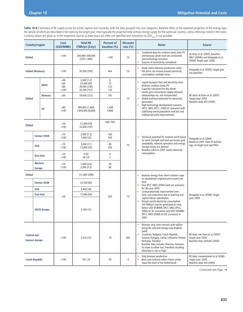
835


Table 10.8 | Summary of RE supply curves for world, regions and countries, with the data grouped into cost categories. Baseline refers to the expected projection of the energy type, the details of which are described in the notes by the target year; most typically the projected total primary energy supply for the particular country, unless otherwise noted in the notes. Currency values are given as in the respective sources as base years are often not specifi ed and conversion to USD2005 is not possible.

Country/regionCost

(USD/MWh)Total RE

(TWh/yr) [EJ/yr]Percent of

baseline (%)Discount rate (%)

Notes Source

Global<100 200,000–300,000

[720–1,080]>100 10

• Combined data for onshore wind, solar PV and biomass given land use constraints and technology scenarios

• Sources of uncertainty considered

de Vries et al. (2007), baseline: WEC (2004b) and Hoogwijk et al. (2004). Target year: 2050

Global (Biomass) <100 97,200 [350] N/A 10• Study claims biomass production under

this price can exceed present electricity consumption multiple times

Hoogwijk et al. (2003). Target year not specifi ed

Global

Wind

<40<60<80<100

2,000 [7.2]23,000 [83]39,000 [140]42,000 [151]

672123133

10

• Liquid transport fuel and electricity from biomass, onshore wind, PV

• Capacity calculated for the whole world; grid connections, supply-demand relationships etc. not incorporated

• Global technical potential for electricity generation

• High technology development scenario (IPCC SRES (IPCC, 2000) A1 scenario) with stabilizing world population and fast and widespread yield improvements.

RE data: de Vries et al. (2007)Target year: 2050Baseline data: IEA (2003)

Biomass <60 59,000 [212] 187

PV<80<100

400,000 [1,440]1,850,000 [6,660]

1,2685,868

Global<70<100

21,000 [76] 53,000 [191]

600–700

-

10

• Technical potential for onshore wind based on wind strength and land use issues; grid availability, network operation and energy storage issues are ignored

• Baseline refers to 2001 world electricity consumption

Hoogwijk et al. (2004)Based on 2001 state of technol-ogy, no target year specifi ed.

Former USSR<70<100

2,000 [7.2]7,000 [25]

160550

USA<70<100

3,000 [11]13,000 [47]

80350

East Asia<70<100

0 [0]50 [.2]

03

Western

Europe

<70<100

1,000 [3.6]2,000 [7.2]

4080

Global

<50

121,805 [438]

N/A 10

• Biomass energy from short-rotation crops on abandoned cropland and unused rest land

• Four IPCC SRES (2000) land use scenarios for the year 2050

• Land productivity improvement over time, cost reductions due to learning and capital-labour substitution

• Present world electricity consumption (20 PWh/yr) may be generated at costs below USD 45/MWh (IPCC SRES (IPCC, 2000) A1 B1 scenarios) and USD 50/MWh (IPCC SRES (2000) A2 B2 scenarios) in 2050

Hoogwijk et al. (2009). Target year: 2050

Former USSR 23,538 [85]

USA 9,444 [34]

East Asia 17,666 [64]

OECD Europe 3,194 [12]

Central and

Eastern Europe<100 3,233 [12] 74 N/A

• Biomass only, best scenario with willow being the selected energy crop (highest yield)

• Countries: Bulgaria, Czech Republic, Estonia, Hungary, Latvia, Lithuania, Poland, Romania, Slovakia

• Baseline data includes Slovenia, however, its share is rather low, therefore resulting distortion is not so high.

RE data: van Dam et al. (2007)Target year: 2030Baseline data: Solinski (2005)

Czech Republic <100 101 [.4] 20 4• Only biomass production• Best-case scenario where future yields

equal the level of the Netherlands

RE data: Lewandowski et al (2006)Target year: 2030Baseline data: IEA (2005)

Continued next Page

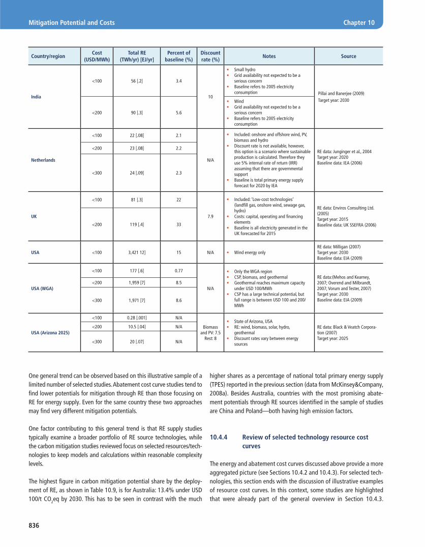
836


One general trend can be observed based on this illustrative sample of a limited number of selected studies. Abatement cost curve studies tend to fi nd lower potentials for mitigation through RE than those focusing on RE for energy supply. Even for the same country these two approaches may fi nd very different mitigation potentials.

One factor contributing to this general trend is that RE supply studies typically examine a broader portfolio of RE source technologies, while the carbon mitigation studies reviewed focus on selected resources/tech-nologies to keep models and calculations within reasonable complexity levels.

The highest fi gure in carbon mitigation potential share by the deploy-ment of RE, as shown in Table 10.9, is for Australia: 13.4% under USD 100/t CO2eq by 2030. This has to be seen in contrast with the much

higher shares as a percentage of national total primary energy supply (TPES) reported in the previous section (data from McKinsey&Company, 2008a). Besides Australia, countries with the most promising abate-ment potentials through RE sources identifi ed in the sample of studies are China and Poland—both having high emission factors.

10.4.4 Review of selected technology resource cost curves

The energy and abatement cost curves discussed above provide a more aggregated picture (see Sections 10.4.2 and 10.4.3). For selected tech-nologies, this section ends with the discussion of illustrative examples of resource cost curves. In this context, some studies are highlighted that were already part of the general overview in Section 10.4.3.

Country/regionCost

(USD/MWh)Total RE

(TWh/yr) [EJ/yr]Percent of

baseline (%)Discount rate (%)

Notes Source

India

<100 56 [.2] 3.4

10

• Small hydro• Grid availability not expected to be a

serious concern• Baseline refers to 2005 electricity

consumption Pillai and Banerjee (2009)Target year: 2030

<200 90 [.3] 5.6

• Wind• Grid availability not expected to be a

serious concern• Baseline refers to 2005 electricity

consumption

Netherlands

<100 22 [.08] 2.1

N/A

• Included: onshore and offshore wind, PV, biomass and hydro

• Discount rate is not available, however, this option is a scenario where sustainable production is calculated. Therefore they use 5% internal rate of return (IRR) assuming that there are governmental support

• Baseline is total primary energy supply forecast for 2020 by IEA

RE data: Junginger et al., 2004 Target year: 2020Baseline data: IEA (2006)

<200 23 [.08] 2.2

<300 24 [.09] 2.3

UK

<100 81 [.3] 22

7.9

• Included: ‘Low-cost technologies’ (landfi ll gas, onshore wind, sewage gas, hydro)

• Costs: capital, operating and fi nancing elements

• Baseline is all electricity generated in the UK forecasted for 2015

RE data: Enviros Consulting Ltd. (2005)Target year: 2015Baseline data: UK SSEFRA (2006)<200 119 [.4] 33

USA <100 3,421 12] 15 N/A • Wind energy onlyRE data: Milligan (2007)Target year: 2030Baseline data: EIA (2009)

USA (WGA)

<100 177 [.6] 0.77

N/A

• Only the WGA region• CSP, biomass, and geothermal• Geothermal reaches maximum capacity

under USD 100/MWh• CSP has a large technical potential, but

full range is between USD 100 and 200/MWh

RE data:(Mehos and Kearney, 2007; Overend and Milbrandt, 2007; Vorum and Tester, 2007)Target year: 2030Baseline data: EIA (2009)

<200 1,959 [7] 8.5

<300 1,971 [7] 8.6

USA (Arizona 2025)

<100 0.28 [.001] N/A

Biomass and PV: 7.5

Rest: 8

• State of Arizona, USA• RE: wind, biomass, solar, hydro,

geothermal• Discount rates vary between energy

sources

RE data: Black & Veatch Corpora-tion (2007)Target year: 2025

<200 10.5 [.04] N/A

<300 20 [.07] N/A

837


Table 10.9 | Summary of carbon abatement cost curves for world, regions and countries (cells including grey literature are coloured in grey).

Country/regionYear

Cost (USD/tCO2eq)

Mitigation potential (Mt CO2)

Percent of baseline (%)

Discount rate (%)

Notes Source

Global 2050 <200 46,195 85 N/A

• Key sensitivities: lower technical potential for wind, hydro or CCS, lower uranium resources raise abatement costs by 2 to 5%

Syri et al. (2008) Baseline model: global ETSAP/TIAMBaseline Scenario: IEA (2009)

Global 2030

<100 6,390 9.1

4

• Scenario A (maximum growth of RE and nuclear)

• Scenario B (50% growth of RE and nuclear)

McKinsey&Company (2009b)

<100 4,070 5.8

Annex I 2020 <100 2,818 20 N/A

• Different abatement allocations analyzed depending (equal marginal cost, per capita emission right convergence, equal percentage reduction)

• CO2 equivalent emissions six Kyoto GHGs, but exclude LULUCF

• Costs in 2005 USD

den Elzen et al. (2009)

Baseline Scenario: IEA WEO (IEA, 2009)

Australia 2020 <100 74 9.5N/A (McKinsey&Company, 2008a)

Australia 2030 <100 105 13

Australia (NSW

Region)2014

<100 8.1 1.0N/A

• New South Wales region

• Includes governmental support for RES

Abatement data: Next Energy (2004)Baseline data: McKinsey&Company (2008a)<300 8.5 1.1

China 2030 <100 1,560 11 4 (McKinsey&Company, 2009a)

China 2030 <50 3,484 27 N/A

• Storylines do not describe all possible development (e.g., disaster scenarios, explicit new climate policies)

• Main abatement (half of total) is effi ciency, the rest is renewable and fuel switch from coal

van Vuuren et al. (2003) Baseline Scenario: ERI 2009

China 2030 <100 2,323 18 N/A

• Main factor infl uencing abatement cost is constraints on the rollout of nuclear power

• Baseline seems to be underestimated as 2010 power consumption is 40% below fact.

Chen, 2005Baseline Scenario: ERI (2009)

Czech Republic 2030

<100 9.3 6.2

N/A• Scenario with maximum

use of RE sourcesMcKinsey&Company (2008b)<200 11.9 8.0

<300 16.6 11

Germany 2020

<100 20 1.9

7

• Societal costs (governmental compensation not included)

McKinsey&Company (2007)<200 31 3.0

<300 34 3.2

Poland 2015<100 50 11

6• Only biomass• Best case scenario

Abatement data: Dornburg et al. (2007)Baseline data: EEA (2007)<200 55.9 12

Continued next Page

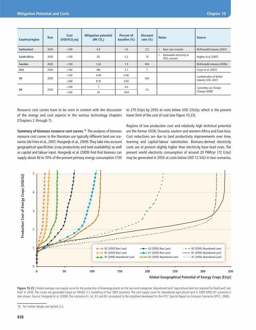
838


Resource cost curves have to be seen in context with the discussion of the energy and cost aspects in the various technology chapters (Chapters 2 through 7).

Summary of biomass resource cost curves.10 The analyses of biomass resource cost curves in the literature use typically different land use sce-narios (de Vries et al., 2007; Hoogwijk et al., 2009). They take into account geographical specifi cities (crop productivity and land availability) as well as capital and labour input. Hoogwijk et al. (2009) fi nd that biomass can supply about 40 to 70% of the present primary energy consumption (130

10 For further details, see Section 2.2.

to 270 EJ/yr) by 2050 at costs below USD 2/GJ/yr, which is the present lower limit of the cost of coal (see Figure 10.23).

Regions of low production cost and relatively high technical potential are the former USSR, Oceania, eastern and western Africa and East Asia. Cost reductions are due to land productivity improvements over time, learning and capital-labour substitution. Biomass-derived electricity costs are at present slightly higher than electricity base-load costs. The present world electricity consumption of around 20 PWh/yr (72 EJ/yr) may be generated in 2050 at costs below USD 12.5/GJ in two scenarios,

Country/regionYear

Cost (USD/tCO2eq)

Mitigation potential (Mt CO2)

Percent of baseline (%)

Discount rate (%)

Notes Source

Switzerland 2030 <100 0.9 1.6 2.5 • Base case scenario McKinsey&Company (2007)

South Africa 2050 <100 83 5.2 10• Renewable electricity to

50% scenarioHughes et al. (2007)

Sweden 2020 <100 1.26 1.9 N/A McKinsey&Company (2008c)

USA 2030 <100 380 3.7 7 Creyts et al. (2007)

UK 2020<100 4.38 0.46

N/AConfederation of British Industry (CBI, 2007)<200 8.76 0.93

UK 2020<100 7 4.0

3.5Committee on Climate Change (2008)<200 33 18.8

Prod

ucti

on C

ost

of E

nerg

y Cr

ops

[USD

/GJ]

1

0

2

3

4

5

Global Geographical Potential of Energy Crops [EJ/yr]

350300250200150100500

A1 (2050) Abandoned LandB1 (2000) Abandoned Land A2 (2050) Abandoned Land

A1 (2050) Rest LandB1 (2050) Rest Land B1 (2050) Abandoned Land

A2 (2050) Rest LandB2 (2050) Rest Land B2 (2050) Abandoned Land

Figure 10.23 | Global average cost-supply curve for the production of bioenergy plants on the two land categories ‘abandoned land’ (agricultural land not required for food) and ‘rest land’ in 2050. The curves are generated based on IMAGE 2.2 modelling of four SRES scenarios. The cost supply curve for abandoned agricultural land in 2000 (SRES B1 scenario) is also shown. Source: Hoogwijk et al. (2009). The scenarios A1, A2, B1 and B2 correspond to the storylines developed for the IPCC Special Report on Emission Scenarios (IPCC, 2000).

839


Figure 10.25 | Resource supply cost curve for PV for four IPCC SRES (IPCC, 2000) sce-narios in 2050. The fi gure also shows the USD 0.1/kWh (USD 0.03/MJ) line used in the paper as the cut-off cost in determining the economic potential (de Vries et al., 2007).

0

1,000

2,000

3,000

4,000

5,000

0 0.1 0.2 0.3 0.4

Production Costs [USD/kWh]

Pote

ntia

l [PW

h/yr

]

2000

A2

B2

A1

B1<USD 0.1 / kWh

Potential for PV

Figure 10.24 | The global technical potential for electricity from biomass in 2000 and in four IPCC SRES (IPCC, 2000) scenarios for 2050 for four production categories (de Vries et al., 2007).

0

20

40

60

80

100

B-2000 A1-B A2-B B1-B B2-BPo

tent

ial [

PWh/

yr]

< USD 0.06/kWh

< USD 0.08/kWh

< USD 0.10/kWh

while below USD 15.3/GJ in two others. At costs of USD 16.7/GJ, about 18 to 53 PWh/yr (65 to 191 EJ/yr) of electricity can be produced in 2050. The global curve that sums all regional curves is found to be relatively fl at up to 300 EJ/yr; land rental costs and the substitution of capital for labour represent the highest sensitivity.

In the study of de Vries et al. (2007), another trade-off is addressed: food versus energy. The authors assess four land use scenarios, each corresponding to different levels of food trade, technology development and population. A low technical potential estimate in the A2 scenario is a direct consequence of more people, hence higher food demand and lower yield (improvement), hence more land demand for food produc-tion (see Figure 10.24).

For a cost range of electricity from biomass of USD 13.9 to 27.8/GJ, there were 7 PWh (25 EJ) of technical potential in the year 2000, while for a projected cost range between USD 8.3 and 27.8/GJ, there is an esti-mated technical potential of 59 PWh (212 EJ) by 2050 (with a sensitivity of 30 to 85 PWh/yr (108 to 310 EJ/yr), depending upon discount rates, land use patterns, technology assumptions and land use implementa-tion fractions).

Summary of PV resource cost curves. De Vries et al. (2007) estimate PV electricity generation technical potential at 4,105 PWh/yr (4,778 EJ/yr) in 2050 at the cost of USD 16.7 to 69.4/GJ. Since the technical poten-tial for the year 2050 depends primarily on cost-reducing innovations, for a cut-off cost level of USD 27.8/GJ, a non-zero technical potential emerges only under specifi c scenario conditions (e.g., high economic growth vs. low population growth, or medium economic and population growth), as in the IPCC (2000) A1 and B1 scenarios (see Figure 10.25).

In this particular study, solar PV economic potential is sensitive to com-petition for land. If the technological breakthroughs do not take place, a large part of the major technical potential is unlikely to become eco-nomic. Its capital-intensive nature also makes it sensitive to changes in discount rates. High or low exclusion factors also affect the solar PV technical potential. For the technical potential, land is not a constraint as even with a high exclusion factor, the technical potential is over 20 times the 2000 world electricity demand (de Vries et al., 2007).

Summary of onshore wind cost curves. Papers assessing wind technical potentials usually base their data on climatic models of wind speeds or interpolation of wind speed measurements (Hoogwijk et al., 2004; de Vries et al., 2007; Changliang and Zhanfeng, 2009). Hoogwijk et al. (2009) have made explicit assumptions about the average turbine availability, wind farm array effi ciency and spacing, and, related to this, power density; this has not differentiated across grid cells, that is, one global parameter has been used. The estimated global technical poten-tial that can be realized at relatively low cost is largely confi ned to three regions (Figure 10.26). These are the USA, the Former USSR and Oceania (Hoogwijk et al., 2004; McElroy et al., 2009). Wind power might even be generated at costs below USD 11.1/GJ in scenarios assuming either high

economic growth and low population growth or medium economic and population growth (IPCC SRES (IPCC, 2000) A1 and B1 scenarios), which is signifi cantly lower than the current cost level (see Chapter 7).

840


Finally, none of the studies reviewed here fully consider transmission and integration issues (see Chapter 8). In one study that did seek to account for these factors, wind remains an important contributor to the worldwide economic potential at less than USD 27.8/GJ, with an eco-nomic potential between 8 and 43 PWh/yr (29 and 155 EJ/yr)—or 50 to 300% of the 2000 world electricity demand (de Vries et al., 2007).

Summary of offshore wind cost curves. For offshore wind, the technical potential and costs are strongly determined by the distance of the installation from the shore and the water depth. In a recent study by EEA (2007), the lower limit of wind speed at hub height has been set to 5.0 m/s to consider the wind power plant economically via-ble. At an average production cost of USD2005 0.024/MJ (6.9 Eurocents/kWh) in 2030, 5,800 GW of offshore wind power could be developed in Europe (Figure 10.27).

Various studies have assessed the technical potential for offshore wind. Nevertheless, only Fellows (2000) presents the assessments at a global level (except Norway and Canada), including cost estimates for the time frame to 2020. Hoogwijk and Graus (2008) have added values for Canada and updated the data for the technological development for 2020 to 2050. High technical potentials are found in OECD Europe and Latin America, the latter having high shares of unexplored low-cost technical potentials. An economic potential of 1.2 PWh/yr (4.3 EJ/yr) for OECD Europe and Latin America is found at costs lower than USD 27.8/GJ. At costs above USD 13.9/GJ, 0.3 PWh/yr (1 EJ/yr) is available in OECD Europe, and 0.55 PWh/yr (1.98 EJ/yr) in Latin America. The lowest techni-cal potentials are found in the Middle East, where even at less than USD

27.8/GJ only 0.18 PWh/yr (0.65 EJ/yr) capacity is available (Hoogwijk and Graus, 2008).

Summary of technology resource cost curves. This section has reviewed selected resource cost curves for selected RE technologies for which such curves were found. It is important to emphasize that such studies are comparable only to a limited extent due to the use of dif-ferent methodologies and potentially confl icting assumptions (such as related to land use), thus they should not be directly used for poten-tial summation or comparison purposes. These results also signifi cantly differ from the integrated technology cost curves produced based on scenarios presented in Section 10.3.2.1, since these present potential deployment levels taking into account many more constraints than the technical potential/cost studies in Section 10.3.

10.4.5 Gaps in knowledge

There is a major gap in knowledge for RE heat and transport fuel tech-nical potentials on a regional basis, especially as a function of cost. Additionally, the real benefi t of the cost curve method (to identify the really cost-effective opportunities) in practice cannot be fully utilized with the given data sets. Average costs for a technology for a whole region mask the really cost-effective technical potentials and sites into an average, compromised by the inclusion of less attractive sites or sub-technologies. Therefore, signifi cant, globally coordinated further research is needed for refi ning these curves into sub-steps by sites and sub-technologies in order to identify the most attractive opportunities

0

0.02

0.04

0.06

0.08

0.10

0.12

0.14

0.16

0.18

0.20

0 5 10 15 20 25

Win

d El

ectr

icit

y Pr

oduc

tion

Cos

ts [U

SD/k

Wh]

Technical Potential [PWh/yr]

Canada

USA

Former USSR

Oceania

OECD Europe

Global

Figure 10.26 | Global, regional and country cost-supply curves for wind energy (USD/kWh versus PWh/yr) (Hoogwijk et al., 2004).

841


Figure 10.27 | Technical potential for offshore wind energy generation at different water depths in 2030 for Europe (EEA, 2009).

0

500

1,000

1,500

2,000

2,500

0.00 0.01 0.02 0.03 0.04 0.05 0.06 0.07 0.08 0.09 0.10 0.11 0.12 0.13 0.14 0.15

Win

d En

ergy

Pot

enti

al [G

W]

40–50 Metres

30–40 Metres

20–30 Metres

0–20 Metres

Costs [EUR/kWh]

broken out of otherwise less economic technologies (such as more attractive wind sites, higher productivity biomass technologies/plants/sites, etc.). Finally, global data sets on deployment rates as a function of energy production costs as well as the cost of additional system bal-ancing and transmission are a key requisite for integrated assessment modelling studies. The lack of such comprehensive data sets (with the laudable exception of Hoogwijk and Graus data) is striking, and is an important knowledge gap.

10.5 Costs of commercialization and deployment

Some RE technologies are broadly competitive with current market energy prices. Many of the other RE technologies can provide compet-itive energy services in certain circumstances, for example, in regions with favourable resource conditions or that lack the infrastructure for other low-cost energy supplies. In most regions of the world, however, policy measures are still required to ensure rapid deployment of many RE sources.

The aforementioned statement, which is consistent with recent publi-cations of the IEA (IEA, 2007a, 2010a,d), is based on a consideration of the resource base, the energy services requested as well as tech-nology-specifi c assessments of current costs of investment, fi nancing, operation and maintenance as presented in the cost sections of the var-ious technology chapters (see Sections 2.7, 3.8, 4.7, 5.8, 6.7 and 7.8).

Under favourable conditions, inter alia, modern combustible biomass to produce heat (IEA, 2007a), solar thermal energy (e.g., solar water heaters in China (IEA, 2010d)), selected off-grid PV applications (IEA, 2010c), large-scale hydropower (IEA, 2008a), larger geothermal

projects (>30 MWe (IEA, 2007b)) and (if the cost of carbon is refl ected in the markets) wind onshore power plants (IEA, 2010a) are already competitive. Provided that suffi cient policy support is available, grid parity of PV (i.e., competitiveness with grid retail prices) is envisioned in many countries by 2020 (IEA, 2010c). Other technologies, such as CSP and offshore wind power, will require further support in order to compete with wholesale prices in the long term.

Currently and in the mid-term, the application of RE technologies can result in additional private costs compared to energy supply from other sources.11 Starting with a review of present technology costs (i.e., current costs observed and published in the last few years), the remainder of this section will focus on expectations about how these costs might decline in the future, for instance, due to extended R&D efforts, technological learning associated with increased deploy-ment, or spill-over effects (see IPCC, 2007). In addition, historic R&D expenditures and future investment needs will be discussed. It must be emphasized that Section 10.5 focuses on technology costs only. Integration aspects are discussed in Chapter 8; externalities and the associated social costs in Chapter 9 and Section 10.6.

10.5.1 Introduction: Review of present technology costs

In the fi eld of RE, energy supply costs are mainly determined by invest-ment costs. Nevertheless, operation and maintenance costs (O&M costs), and—if applicable—fuel costs (in the case of biomass), may play an important role as well. The respective cost components are discussed

11 Within this section, the external costs of other technologies are not considered. Al-though the term ‘private’ will be omitted in the remainder of this section, the reader should be aware that all costs discussed here are private costs in the sense of Section 10.6. Externalities therefore are not taken into account.

842


in detail in the technology chapters (Sections 2.7, 3.8, 4.7, 5.8, 6.7 and 7.8) and recent values are summarized in Annex III (Tables 1 through 3), where, inter alia, technology-specifi c values for typical device sizes (in MW), recent specifi c investment costs (in USD/kW), annual O&M costs (in USD/kW or US cents/kWh), capacity factors (in %) and economic life-times (in years) can be found. At a global scale, the respective values are highly uncertain for the various RE technologies. As recent years have shown, investment costs, for instance, might be considerably infl uenced by changes in material (e.g., steel) and engineering costs as well as by technological learning and mass market effects (IEA, 2010a,b).

Levelized costs of energy (LCOE, also called levelized unit costs or levelized generation costs; see Annex II for more information and illus-trative calculations) are defi ned as ‘the ratio of total lifetime expenses versus total expected outputs, expressed in terms of the present value equivalent’ (IEA, 2005, p.174). LCOE therefore capture the full costs (i.e., investment costs, O&M costs, fuel costs and decommissioning costs) of an energy conversion installation and allocate these costs over the energy output during its lifetime. In general, LCOE do not take into account subsidies, policy incentives or integration costs.

The LCOE that can be derived from the values given in Annex III (Tables 1 to 3) are shown in Figures 10.28 through 10.31. Though these represent LCOE estimates for recent renewable energy plants, LCOE are different at different locations as discount rates, investment cost, O&M costs, capacity factors (especially due to the local RE resource availability) and fuel prices are site dependent (Heptonstall, 2007; IEA, 2010b).

The cost ranges in the background of Figure 10.28 display the global ranges of indicative values for the cost of energy supply options using fossil fuels. For electricity, the range is based on a recent assessment of LCOE for new coal and gas-fi red power plants (IEA, 2010b). The values refer to centralized power plants. In contrast to IEA (2010b), a carbon price mark-up has not been included.

Following IEA (2007a), the (levelized) cost of oil and gas based heat sup-ply options are estimated by taking into account retail fuel prices and conversion losses only. The investment costs for conventional boilers were neglected, because their contribution to overall LCOH is small (and because conventional heating facilities are often needed as a back-up for RE conversion technologies). Retail prices are used as most RE heating technologies have to compete at the fi nal consumer level. For conversion effi ciencies the values proposed by IEA (2007a) are applied. The indicative cost range depicted in Figure 10.28 is based on differing national retail prices (including taxes) for light fuel oil and natural gas as reported in the recently published IEA Key World Energy Statistics (IEA, 2010f). The lower bound of the range refers to natural gas-fi red industrial heating applica-tions; the higher bound to light fuel oil use in households.

According to the IEA (2010d), the cost of conventional transport fuels is strongly correlated with the underlying (historical) Brent crude oil spot price. In order to facilitate an investigation of the competitiveness of bio-fuels in times of highly fl uctuating crude oil prices, the indicative transport

fossil fuel cost range depicted in Figure 10.28 refers to a variation in the underlying crude oil spot price between USD 40 and 130/barrel.

As RE technologies are often characterized by high shares of investment costs relative to O&M costs and fuel costs, the applied discount rate has a prominent infl uence on the LCOE (see Figures 10.29, 10.30 and 10.31). The discount rate itself refers to a risk-free rate of return (assessed to be broadly of the order of 3%/yr) adjusted by a project-dependent risk premium (IEA, 2005, Appendix 6). According to IEA (2010b) (see Chapter 8 in this report), a discount rate of 5% is typically adopted by US investors facing a low risk in a fairly stable environment. Prominent examples are a public monopolist acting in a regulated market or a pri-vate investor investing in a low-risk technology in a favourable market environment. In the case where the investor is facing substantially greater fi nancial, technological and price risks, a real discount rate of 10% can be justifi ed (IEA, 2010b, p.154). As discussed in Appendix II, this report uses three values of real discount rates (3, 7 and 10%) in order to allow for an easy comparison between different projects and/or technologies. Note that in liberalized markets, private investors might ask for a higher real rate of returns than those characterized by a discount rate of 10% (IEA, 2005). The LCOE ranges depicted in Figures 10.28 through 10.31 can be traced back to variations in the underlying parameters, which, in turn, can be grouped into:

a) The considered range of the performance parameter (characterized by the capacity factor) that heavily depends on the local resource base (e.g., wind velocities or solar radiation).

b) The global spread of the technology-dependent parameters (i.e., life-time as well as investment and O&M costs) that are infl uenced by local technology maturity, market conditions and wages.

c) The range of the different real discount rate selected for this study (3 to 10%).

The lowest LCOE values depicted in Figures 10.28 through 10.31 cor-respond to best-case conditions (highest achievable capacity factor and highest lifetime, lowest investment and O&M costs, and lowest bound on the discount rate). The upper range of the LCOE is characterized by high, but still reasonable values for costs; low, but still realistic values for the lifetime; low, but still observed capacity factors; and a discount rate of 10% (if not indicated otherwise). Less favourable conditions can yield sub-stantially higher costs compared to those shown in the fi gures. The results presented in Figures 10.28 through 10.31 warrant some discus-sion in comparison to the cost data presented in other chapters. Most of the technology chapters show the levelized cost as a function of a) the capacity factor, b) the investment costs and c) the discount rate (Sections 2.7, 3.8, 4.6, 5.8, 6.7 and 7.8). In order to facilitate a comparison between different technologies, Figures 10.28 through 10.31 do not repeat show-ing the respective sensitivities in an explicit way. As discussed above, the

843


Range of Oil and Gas Based Heating Cost

Range of Non-Renewable Electricity Cost

Range of Gasoline and Diesel Cost

[UScent2005 /kWh]

0 10 20 30 40 50 60 70 80 90 100

[USD2005 /GJ]

Biofuels

Geothermal Heat

Solar Thermal Heat

Biomass Heat

Wind Electricity

Ocean Electricity

Hydropower

Geothermal Electricity

Solar Electricity

Biomass Electricity

27525022520017515012510075500 25

Non-Renewables

Heat

Transport Fuels

Electricity

Lower Bound

Upper Bound

Medium Values

Biofuels:1. Corn ethanol2. Soy biodiesel3. Wheat ethanol4. Sugarcane ethanol

5. Palm oil biodiesel

Biomass Heat:1. Municipal solid waste based CHP2. Anaerobic digestion based CHP3. Steam turbine CHP4. Domestic pellet heating system

Solar Thermal Heat:1. Domestic hot water systems in China2. Water and space heating

Geothermal Heat:1. Greenhouses2. Uncovered aquaculture ponds3. District heating4. Geothermal heat pumps5. Geothermal building heating

Biomass:1. Cofiring2. Small scale combined heat and power, CHP (Gasification internal combustion engine)3. Direct dedicated stoker & CHP4. Small scale CHP (steam turbine)5. Small scale CHP (organic Rankine cycle)

Solar Electricity:1. Concentrating solar power2. Utility-scale PV (1-axis and fixed tilt) 3. Commercial rooftop PV4. Residential rooftop PV

Geothermal Electricity:1. Condensing flash plant2. Binary cycle plant

Hydropower:1. All types

Ocean Electricity:1. Tidal barrage

Wind Electricity:1. Onshore2. Offshore

Transport FuelsHeatElectricity

Notes: Medium values are shown for the following subcategories, sorted in the order as they appear in the respective ranges (from left to right):

The lower range of the levelized cost of energy for each RE technology is based on a combination of the most favourable input-values, whereas the upper range is based on a combination of the least favourable input values. Reference ranges in the figure background for non-renewable electricity options are indicative of the levelized cost of centralized non-renewable electricity generation. Reference ranges for heat are indicative of recent costs for oil and gas based heat supply options. Reference ranges for transport fuels are based on recent crude oil spot prices of USD 40 to 130/barrel and corresponding diesel and gasoline costs, excluding taxes.

Figure 10.28 | Range in recent levelized cost of energy for selected commercially available RE technologies in comparison to recent non-renewable energy costs. Technology subcategories and discount rates were aggregated for this fi gure. For related fi gures with less or no such aggregation, see Annex III. Additional information concerning the cost of non-renewable energy supply options is given below.

844


fi gures nevertheless show the range of LCOE that originates from varying the capacity factors and investment costs within reasonable bounds.

In contrast to the aforementioned LCOE sensitivity diagrams that are contained in the technology chapters, the supply cost curves presented in Section 10.4.4 (Figures 10.23, 10.25, 10.26 and 10.27) provide addi-tional information about the available resource base. Instead of showing the sensitivity with respect to the capacity factor, they allow an insight into the amount of RE that can be harnessed up to a prescribed level of the

0 10 20 30 40 50 60 70 80 90

Bioenergy (Direct Dedicated & Stoker CHP)

Bioenergy (Co-Firing)

Bioenergy (Small Scale CHP, ORC)

Bioenergy (Small Scale CHP, Steam Turbine)

Bioenergy (Small Scale CHP, Gasification ICE)

Solar PV (Residential Rooftop)

Solar PV (Commercial Rooftop)

Solar PV (Utility Scale, Fixed Tilt)

Solar PV (Utility Scale, 1-Axis)

Concentrating Solar Power

Geothermal Energy (Condensing-Flash Plants)

Geothermal Energy (Binary-Cycle Plants)

Hydropower

Ocean Energy (Tidal Range)

Wind Energy (Onshore, Large Turbines)

Wind Energy (Offshore, Large Turbines)

[UScent2005 /kWh]

3% Discount Rate

7% Discount Rate

10% Discount Rate

Figure 10.29 | Levelized cost of electricity for commercially available RE technologies at 3, 7 and 10% discount rates. The levelized cost estimates for all technologies are based on input data summarized in Annex III and the methodology outlined in Annex II. The lower bound of the levelized cost range is based on the low ends of the ranges of investment, operations and maintenance (O&M), and (if applicable) feedstock cost and the high ends of the ranges of capacity factors and lifetimes as well as (if applicable) the high ends of the ranges of conversion effi ciencies and by-product revenue. The higher bound of the levelized cost range is accordingly based on the high end of the ranges of investment, O&M and (if applicable) feedstock costs and the low end of the ranges of capacity factors and lifetimes as well as (if applicable) the low ends of the ranges of conversion effi ciencies and by-product revenue. Note that conversion effi ciencies, by-product revenue and lifetimes were in some cases set to standard or average values. For data and supplementary information see Annex III. (CHP: combined heat and power; ORC: organic Rankine cycle, ICE: internal combustion engine).

LCOE. This additional information comes from studies that made their own assumptions about other factors (beyond site-dependent capacity factors) that have an infl uence on the LCOE (e.g., discount rates, investment and O&M costs, and lifetimes). As a result, these results might not be fully com-patible with the LCOE calculations summarized in Annex III. The supply cost curves discussed in Section 10.3.2.1 (Figures 10.15 through 10.17) exhibit the amount of RE that is harnessed (once again as a function of the associated LCOE) in different regions once specifi c

845


Figure 10.30 | Levelized cost of heat (LCOH) for commercially available RE technologies at 3, 7 and 10% discount rates. The LCOH estimates for all technologies are based on input data summarized in Annex III and the methodology outlined in Annex II. The lower bound of the levelized cost range is based on the low ends of the ranges of investment, operations and maintenance (O&M), and (if applicable) feedstock cost and the high ends of the ranges of capacity factors and lifetimes as well as (if applicable) the high ends of the ranges of conversion effi ciencies and by-product revenue. The higher bound of the levelized cost range is accordingly based on the high end of the ranges of investment, O&M and (if applicable) feedstock costs and the low end of the ranges of capacity factors and lifetimes as well as (if applicable) the low ends of the ranges of conversion effi ciencies and by-product revenue. Note that capacity factors and lifetimes were in some cases set to standard or average values. For data and supplementary information see Annex III. (MSW: municipal solid waste; DHW: domestic hot water).

0 50 100 150 200

Biomass (Domestic Pellet Heating)

Biomass (MSW, CHP)

Biomass (Steam Turbine, CHP)

Biomass (Anaerobic Digestion, CHP)

Solar Thermal Heating (DHW, China)

Solar Thermal Heating (DHW,Thermo-Siphon, Combi)

Geothermal (Building Heating)

Geothermal (District Heating)

Geothermal (Greenhouses)

Geothermal (Aquaculture Ponds,Uncovered)

Geothermal Heat Pumps (GHP)

[USD2005 /GJ]

3% Discount Rate

7% Discount Rate

10% Discount Rate

trajectories for the expansion of RE are followed. As the results clearly show, the respective numbers are heavily dependent on the peculiarities (e.g., applied assumptions) of the underlying models.

In addition, it must be emphasized that most of the supply cost curves refer to future points in time (e.g., 2030 or 2050), whereas the levelized costs given in the cost sections of the technology chapters as well as those shown in Figures 10.28 through 10.31 (and in Annex III) refer to current costs.

The LCOE presented in Figures 10.28 through 10.31 are based on literature reviews and represent the most current cost data available. The correspond-ing data are summarized in Tables 1 to 3 of Annex III. The LCOE ranges are rather broad as the values vary across the globe depending on the RE resource base and the local costs of investment, fi nancing, operation and maintenance. Comparison between different technologies therefore should not be based on the cost data provided here; instead, site-, proj-ect- and investor-specifi c conditions should be taken into account. The technology chapters (Sections 2.7, 3.8, 4.6, 5.8, 6.7 and 7.8) provide useful sensitivities in this respect.

Similar to LCOE, wholesale and retail prices of electricity that might be used in order to assess the competitiveness of centralized and decentralizedRE power plants are country specifi c as well. The same holds true for the cost of fuels used for heating and transport purposes. A comparison of RE LCOE with those of other technologies or market prices should therefore be project-based as well.

The LCOE of a technology is not the sole determinant of its value or economic competitiveness. In addition to integration and transmission costs, relative environmental impacts must be considered, as well as the contribution of a technology to meeting specifi c energy services, for example, peak electricity demands.

Nevertheless, and despite the existing uncertainties, summarizing the information contained in Figures 10.28 through 10.31, Sections 2.7, 3.8, 4.6, 5.8, 6.7 and 7.8 as well as in recent benchmark studies (IEA, 2010a,b,c,d), the following conclusions can be drawn:

A comparison of LCOE of RE technologies with those of other technolo-gies (nuclear, gas and coal power plants) shows that—at least as long as

846


Figure 10.31 | Levelized cost of fuels (LCOF) for commercially available biomass conversion technologies at 3, 7 and 10% discount rates. LCOF estimates for all technologies are based on input data summarized in Annex III and the methodology outlined in Annex II. The lower bound of the levelized cost range is based on the low ends of the ranges of investment, operations and maintenance (O&M) and feedstock costs. The higher bound of the levelized cost range is accordingly based on the high end of the ranges of investment, O&M and feedstock costs. Note that conversion effi ciencies, by-product revenue, capacity factors and lifetimes were set to average values. For data and supplementary information see Annex III. (HHV: higher heating value).

[USD/GJHHV]

0 10 20 30 40 50 60

Ethanol - Sugarcane

Ethanol - Corn

Ethanol - Wheat

Biodiesel - Soy Oil

Biodiesel - Palm Oil

3% Discount Rate

7% Discount Rate

10% Discount Rate

externalities are not taken into account—RE sources are often not yet com-petitive with other sources, especially if they both feed into the electricity grid. If the respective technologies are used in a decentralized mode, private investors would compare their production cost with the retail consumer power price, which is much higher. In this case, niche markets might exist that facilitate the market introduction of new technologies. The same holds true for applications in remote areas, where often no grid-based electricity is available (IEA, 2010c). Similar trends exist outside of the power sector for the use of RE in heating and transportation applications (IEA, 2007a).

Given suitable conditions, the lower end of the LCOE ranges indicate (see Figure 10.28) that some RE technologies already can compete with tradi-tional forms at current energy market prices in many regions of the world. That said, the graphs provide no indication of the resource potential that can be utilized at low cost. Sections 10.3 and 10.4 provide more informa-tion in this regard.

10.5.2 Prospects for cost decreases

In the fi eld of RE, signifi cant opportunities exist to further improve the energy effi ciencies and/or to decrease the costs of producing and installing the respective technologies (see Sections 2.7, 3.8, 4.7, 6.7 and 7.8). Together, these effects are expected to decrease the

LCOE of many innovative RE sourcing technologies in the future (IEA, 2008b, 2010a). According to Junginger et al. (2006), the list of the most important mechanisms causing cost reductions comprises:

• Learning by searching, that is, improvements due to research, devel-opment and demonstration (RD&D)—especially, but not exclusively in the stage of invention;

• Learning by doing (in the strict sense), that is, improvements in the production process (e.g., increased labour effi ciency, work specialization);

• Learning by using, that is, improvements triggered by user experi-ence feedbacks occur once the technology enters (niche) markets;

• Learning by interacting (or ‘spill-overs’) (IPCC, 2007; Clarke et al., 2008), that is, the reinforcement of the above-mentioned mecha-nism due to an increased interaction among various actors in the diffusion phase;

• Upsizing of technologies (e.g., up-scaling of wind turbines); and

• Economies of scale (i.e., mass production) once the stage of large-scale production is reached.

847


The various mechanisms may occur simultaneously at various stages of the innovation chain. In addition, they may reinforce each other. As a consequence of the aforementioned mechanisms, many technologies applied in the fi eld of RE sources showed a signifi cant cost decrease in the past (IEA, 2000, 2008a). This empirical observation is highlighted by experience (or ‘learning’) curves, which describe how costs have declined with accumulated experience and corresponding cumulative production or installed capacity. An illustrative experience curve (referring to wind energy) is shown in Figure 10.32. Further examples concerning bioen-ergy use and photovoltaic modules can be found in Section 2.7.2 (Figure 2.21) and in Section 3.8.3 (Figure 3.17), respectively.

For a doubling of the (cumulatively) installed capacity, many technolo-gies showed a more or less constant percentage decrease in the specifi c investment costs (or in the levelized costs or unit price, depending on the selected cost indicator). The corresponding learning rate (LR) is defi ned as the percentage cost reduction for each doubling of the cumulative capacity. A summary of observed learning rates is provided in Table 10.10. Occasionally, the progress ratio (PR) is used as a substitute for the learning rate. It is defi ned as PR = 1 - LR (e.g., a learning rate of 20% would imply a progress ratio of 80%). Frequently, energy supply costs (e.g., electricity generation costs) and the cumulative energy supplied

by the respective technology (e.g., the cumulative electricity produc-tion) are used as substitutes for investment costs and the cumulative installed capacity, respectively. If the learning rate is time-independent, the empirical experience curve can be fi tted by a power law. In this case, representing costs against cumulative installed capacity in a graph with double logarithmic scales shows the experience curve as a straight line (Junginger et al., 2010) (see Figure 10.32).

As there is no natural law that costs have to follow a power law (Junginger et al., 2010), care must be taken if historic experience curves are extrapolated in order to predict future costs (Nemet, 2009). Obviously, the cost reduction cannot go ad infi nitum and there might be some unexpected steps in the curve in practice (e.g., caused by tech-nology breakthroughs). As technologies mature, learning rates may fall (Ferioli et al., 2009; Nemet, 2009). In order to avoid implausible results, projections that extrapolate experience cost curves in order to assess future costs should therefore constrain the cost reduction by appropriate fl oor costs (see Edenhofer et al., 2006).

Concerning levelized costs or turnkey investment costs, a signifi cant share of these fl oor costs might arise from balance of system and installation costs, which, in turn, are often dominated by labour costs. Although installers might gain experience, the future decrease in this cost component is limited (Yang, 2010). Unfortunately, cost data are not easily obtained in a competitive market environment. Indicators that are intended to serve as a substitute, for example, product prices, do not necessarily reveal the actual improvement achieved (Yu et al., 2011). Instead, they might be heavily infl uenced by an imbalance of supply and demand. This refers to both the fi nal product itself (e.g., if fi nancial sup-port stipulates a high demand) and the cost of production factors, which might be temporarily scarce (e.g., steel prices due to supply bottlenecks). A deviation from price-based experience curves, as especially observed for PV modules in the years between 2004 and 2008 (see Section 3.8.3, Figure 3.17), therefore does not necessarily imply that a fundamental cost limit has been reached (Nemet, 2009). Instead, it might simply indicate that producers were able to make extra profi ts while the cost reduction takes place in the background. After a subsequent ‘shakeout’ phase, the short-term deviation from the long-term experience curve might be largely removed (Junginger et al., 2005b). In the fi eld of solar PV, for instance, the recent development is characterized by overcapaci-ties and a resulting increased competition between PV companies (see Chapter 3). As a result, PV system prices fell by 40% between 2008 and 2009 (IEA, 2010c; and see Section 3.8.3, Figure 3.17).

A summary of observed learning rates is provided in Table 10.10. Learning rates referring to investment costs (or turnkey investment costs) are often lower than those derived from electricity generation costs. Although the cost reduction in the specifi c investment costs of wind power plants, for instance, might be small, the scale-up results in higher hub heights and an associated signifi cant increase in the capac-ity factor (and consequently in the amount of energy delivered). The ultimate goal of technological progress in the fi eld of RE is a reduction of the energy production costs per kWh (in other words, the LCOE), not of the investment costs per se (see Section 7.8.4.1; EWEA, 2009; Ferioli et al., 2009). Any efforts to assess future costs by extrapolating historic experience curves must take into account the uncertainty of learning rates as well as the caveats and knowledge gaps discussed in Sections 10.5.6 and 7.8.4.1. As a supplementary approach, expert elicitations could be used to gather additional information about future cost reduction potentials (Curtright et al., 2008), which might be contrasted with the assessments gained by using learning rates. Furthermore, engineering model analy-ses to identify technology improvement potentials could also provide additional information for developing cost projections (see Sections 2.6, 3.7, 4.6, 6.6 and 7.7)

Important potential technological advances and associated cost reductions, for instance, are expected in (but are not limited to) the fol-lowing application fi elds: next-generation biofuels and bio-refi neries (see Section 2.6); advanced PV and CSP technologies and manufacturing processes (see Section 3.7); enhanced geothermal systems (see Section

Figure 10.32 | Illustrative experience curve for wind turbines. Source: Nemet (2009).

Win

d Po

wer

Pri

ce [U

SD20

06 /W

]

10 100 1000 10,000 100,000Cumulative Capacity [MW]

1981

1990

2000 2006

10

1

848


Table 10.10 | Observed learning rates for various electricity supply technologies. Source: IEA, 2008b, p. 205, extended and updated with a select list of additional literature (this report). (Note that values cited by older publications are less reliable as these refer to shorter time periods. In addition, only values for single-factor learning curves are shown. As a consequence there is some, albeit restricted, overlap with the learning rate information offered by Chapters 2 through 7.)

Technology Source Country / region Period Learning rate (%) Performance measure

Onshore wind

Neij, 1997 Denmark 1982-1995 4 Price of wind turbine (USD/kW)

Mackay and Probert, 1998 USA 1981-1996 14 Price of wind turbine (USD/kW)


Durstewitz, 1999 Germany 1990-1998 8 Price of wind turbine (USD/kW)

IEA, 2000 USA 1985-1994 32 Electricity production cost (USD/kWh)

IEA, 2000 EU 1980-1995 18 Electricity production cost (USD/kWh)

Kouvaritakis et al., 2000 OECD 1981-1995 17 Price of wind turbine (USD/kW)


Junginger et al., 2005a Spain 1990-2001 15 Turnkey investment costs (EUR/kW)

Junginger et al., 2005a UK 1992-2001 19 Turnkey investment costs (EUR/kW)

Söderholm and Sundqvist, 2007 Germany, UK,Denmark

1986-2000 5 Turnkey investment costs (EUR/kW)

Neij, 2008 Denmark 1981-2000 17 Electricity production cost (USD/kWh)

Kahouli-Brahmi, 2009 Global 1979-1997 17 Investment costs (USD/kW)

Nemet, 2009 Global 1981-2004 11 Investment costs (USD/kW)

Wiser and Bolinger, 2010 Global 1982-2009 9 Investment costs (USD/kW)

Offshore wind

Isles, 2006 8 EU countries 1991-2006 3 Investment cost of wind farms (USD/kW)

Photovoltaics (PV)

Harmon, 2000 Global 1968-1998 20 Price PV module (USD/Wpeak)

IEA, 2000 EU 1976-1996 21 Price PV module (USD/Wpeak)

Williams, 2002 Global 1976-2002 20 Price PV module (USD/Wpeak)

ECN, 2004 EU 1976-2001 20-23 Price PV module (USD/Wpeak)

ECN, 2004 Germany 1992-2001 22 Price of balance of system costs

van Sark et al., 2007 Global 1976-2006 21 Price PV module (USD/Wpeak)

Kruck and Eltrop, 2007 Germany 1977-2005 13 Price PV module (EUR/Wpeak)

Kruck and Eltrop, 2007 Germany 1999-2005 26 Price of balance of system costs

Nemet, 2009 Global 1976-2006 15-21 Price PV module (USD/Wpeak)

Concentrating Solar Power (CSP)

Enermodal, 1999 USA 1984-1998 8-15 Plant investment cost (USD/kW)

Biomass

IEA, 2000 EU 1980-1995 15 Electricity production cost (USD/kWh)

Goldemberg et al., 2004 Brazil 1985-2002 29 Prices for ethanol fuel (USD/m3)

Junginger et al., 2005b Sweden, Finland 1975-2003 15 Forest wood chip prices (EUR/GJ)

Junginger et al., 2006 Denmark 1984-1991 15 Biogas production costs (EUR/Nm3)

Junginger et al., 2006 Sweden 1990-2002 8-9 Biomass CHP power (EUR/kWh)

Junginger et al., 2006 Denmark 1984-2001 0-15 Biogas production costs (EUR/Nm3)

Junginger et al., 2006 Denmark 1984-1998 12 Biogas plants (€/m3 biogas/day )

Van den Wall Bake et al., 2009 Brazil 1975-2003 19 Ethanol from sugarcane (USD/m3)

Goldemberg et al., 2004 Brazil 1980-1985 7 Ethanol from sugarcane (USD/m3)

Goldemberg et al., 2004 Brazil 1985-2002 29 Ethanol from sugarcane (USD/m3)

Van den Wall Bake et al., 2009 Brazil 1975-2003 20 Ethanol from sugarcane (USD/m3)

Hettinga et al., 2009 USA 1983-2005 18 Ethanol from corn (USD/m3)

Hettinga et al., 2009 USA 1975-2005 45 Corn production costs (USD/t corn)

Van den Wall Bake et al., 2009 Brazil 1975-2003 32 Sugarcane production costs (USD/t)

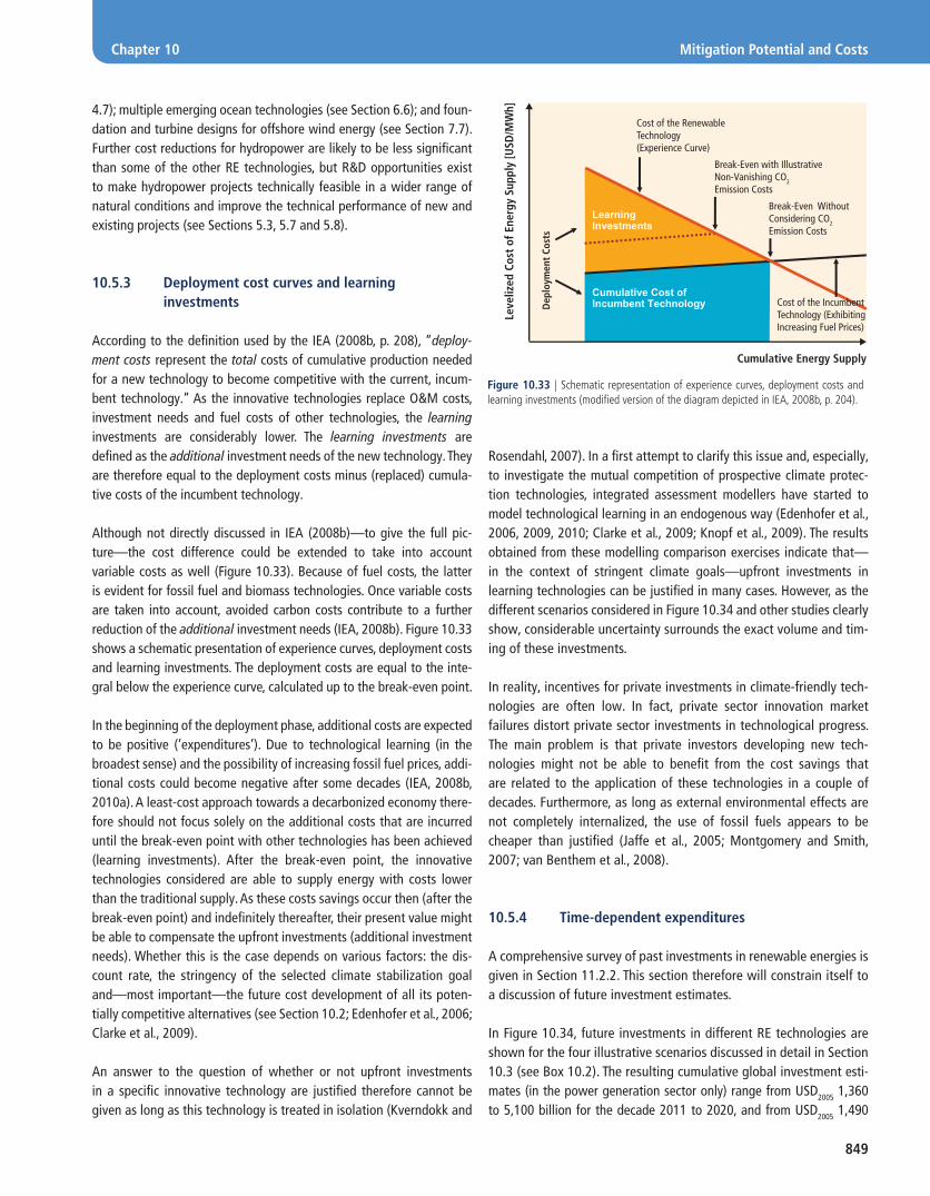
849


Rosendahl, 2007). In a fi rst attempt to clarify this issue and, especially, to investigate the mutual competition of prospective climate protec-tion technologies, integrated assessment modellers have started to model technological learning in an endogenous way (Edenhofer et al., 2006, 2009, 2010; Clarke et al., 2009; Knopf et al., 2009). The results obtained from these modelling comparison exercises indicate that—in the context of stringent climate goals—upfront investments in learning technologies can be justifi ed in many cases. However, as the different scenarios considered in Figure 10.34 and other studies clearly show, considerable uncertainty surrounds the exact volume and tim-ing of these investments.

In reality, incentives for private investments in climate-friendly tech-nologies are often low. In fact, private sector innovation market failures distort private sector investments in technological progress. The main problem is that private investors developing new tech-nologies might not be able to benefi t from the cost savings that are related to the application of these technologies in a couple of decades. Furthermore, as long as external environmental effects are not completely internalized, the use of fossil fuels appears to be cheaper than justifi ed (Jaffe et al., 2005; Montgomery and Smith, 2007; van Benthem et al., 2008).

10.5.4 Time-dependent expenditures

A comprehensive survey of past investments in renewable energies is given in Section 11.2.2. This section therefore will constrain itself to a discussion of future investment estimates.

In Figure 10.34, future investments in different RE technologies are shown for the four illustrative scenarios discussed in detail in Section 10.3 (see Box 10.2). The resulting cumulative global investment esti-mates (in the power generation sector only) range from USD2005 1,360 to 5,100 billion for the decade 2011 to 2020, and from USD2005 1,490

4.7); multiple emerging ocean technologies (see Section 6.6); and foun-dation and turbine designs for offshore wind energy (see Section 7.7). Further cost reductions for hydropower are likely to be less signifi cant than some of the other RE technologies, but R&D opportunities exist to make hydropower projects technically feasible in a wider range of natural conditions and improve the technical performance of new and existing projects (see Sections 5.3, 5.7 and 5.8).

10.5.3 Deployment cost curves and learning investments

According to the defi nition used by the IEA (2008b, p. 208), “deploy-ment costs represent the total costs of cumulative production needed for a new technology to become competitive with the current, incum-bent technology.” As the innovative technologies replace O&M costs, investment needs and fuel costs of other technologies, the learning investments are considerably lower. The learning investments are defi ned as the additional investment needs of the new technology. They are therefore equal to the deployment costs minus (replaced) cumula-tive costs of the incumbent technology.

Although not directly discussed in IEA (2008b)—to give the full pic-ture—the cost difference could be extended to take into account variable costs as well (Figure 10.33). Because of fuel costs, the latter is evident for fossil fuel and biomass technologies. Once variable costs are taken into account, avoided carbon costs contribute to a further reduction of the additional investment needs (IEA, 2008b). Figure 10.33 shows a schematic presentation of experience curves, deployment costs and learning investments. The deployment costs are equal to the inte-gral below the experience curve, calculated up to the break-even point.

In the beginning of the deployment phase, additional costs are expected to be positive (‘expenditures’). Due to technological learning (in the broadest sense) and the possibility of increasing fossil fuel prices, addi-tional costs could become negative after some decades (IEA, 2008b, 2010a). A least-cost approach towards a decarbonized economy there-fore should not focus solely on the additional costs that are incurred until the break-even point with other technologies has been achieved (learning investments). After the break-even point, the innovative technologies considered are able to supply energy with costs lower than the traditional supply. As these costs savings occur then (after the break-even point) and indefi nitely thereafter, their present value might be able to compensate the upfront investments (additional investment needs). Whether this is the case depends on various factors: the dis-count rate, the stringency of the selected climate stabilization goal and—most important—the future cost development of all its poten-tially competitive alternatives (see Section 10.2; Edenhofer et al., 2006; Clarke et al., 2009).

An answer to the question of whether or not upfront investments in a specifi c innovative technology are justifi ed therefore cannot be given as long as this technology is treated in isolation (Kverndokk and

Cumulative Cost of Incumbent Technology

Learning Investments

Cost of the Incumbent Technology (Exhibiting Increasing Fuel Prices)

Break-Even with IllustrativeNon-Vanishing CO2 Emission Costs

Cost of the Renewable Technology(Experience Curve)

Cumulative Energy Supply

Leve

lized

Cos

t of

Ene

rgy

Supp

ly [U

SD/M

Wh]

Break-Even Without Considering CO2 Emission Costs

Dep

loym

ent

Cost

s

Figure 10.33 | Schematic representation of experience curves, deployment costs and learning investments (modifi ed version of the diagram depicted in IEA, 2008b, p. 204).

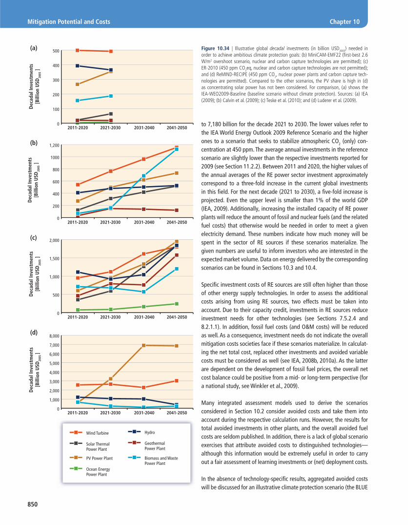
850


to 7,180 billion for the decade 2021 to 2030. The lower values refer to the IEA World Energy Outlook 2009 Reference Scenario and the higher ones to a scenario that seeks to stabilize atmospheric CO2 (only) con-centration at 450 ppm. The average annual investments in the reference scenario are slightly lower than the respective investments reported for 2009 (see Section 11.2.2). Between 2011 and 2020, the higher values of the annual averages of the RE power sector investment approximately correspond to a three-fold increase in the current global investments in this fi eld. For the next decade (2021 to 2030), a fi ve-fold increase is projected. Even the upper level is smaller than 1% of the world GDP (IEA, 2009). Additionally, increasing the installed capacity of RE power plants will reduce the amount of fossil and nuclear fuels (and the related fuel costs) that otherwise would be needed in order to meet a given electricity demand. These numbers indicate how much money will be spent in the sector of RE sources if these scenarios materialize. The given numbers are useful to inform investors who are interested in the expected market volume. Data on energy delivered by the corresponding scenarios can be found in Sections 10.3 and 10.4.

Specifi c investment costs of RE sources are still often higher than those of other energy supply technologies. In order to assess the additional costs arising from using RE sources, two effects must be taken into account. Due to their capacity credit, investments in RE sources reduce investment needs for other technologies (see Sections 7.5.2.4 and 8.2.1.1). In addition, fossil fuel costs (and O&M costs) will be reduced as well. As a consequence, investment needs do not indicate the overall mitigation costs societies face if these scenarios materialize. In calculat-ing the net total cost, replaced other investments and avoided variable costs must be considered as well (see IEA, 2008b, 2010a). As the latter are dependent on the development of fossil fuel prices, the overall net cost balance could be positive from a mid- or long-term perspective (for a national study, see Winkler et al., 2009).

Many integrated assessment models used to derive the scenarios considered in Section 10.2 consider avoided costs and take them into account during the respective calculation runs. However, the results for total avoided investments in other plants, and the overall avoided fuel costs are seldom published. In addition, there is a lack of global scenario exercises that attribute avoided costs to distinguished technologies—although this information would be extremely useful in order to carry out a fair assessment of learning investments or (net) deployment costs.

In the absence of technology-specifi c results, aggregated avoided costs will be discussed for an illustrative climate protection scenario (the BLUE

2011-2020 2021-2030 2031-2040 2041-2050

2011-2020 2021-2030 2031-2040 2041-2050

2011-2020 2021-2030 2031-2040 2041-2050

2011-2020 2021-2030 2031-2040 2041-20500

100

200

300

400

500

Wind Turbine

Solar Thermal Power Plant

PV Power Plant

Ocean Energy Power Plant

Hydro

Geothermal Power Plant

Biomass and Waste Power Plant

0

200

400

600

800

1000

1,200

0

500

1,000

1,500

2,000

0

1,000

2,000

3,000

4,000

5,000

6,000

7,000

8,000

Dec

adal

Inve

stm

ents

[Bill

ion

USD

2005

]D

ecad

al In

vest

men

ts[B

illio

n U

SD20

05 ]

Dec

adal

Inve

stm

ents

[Bill

ion

USD

2005

]D

ecad

al In

vest

men

ts[B

illio

n U

SD20

05 ]

(d)

(c)

(b)

(a) Figure 10.34 | Illustrative global decadal investments (in billion USD2005) needed in order to achieve ambitious climate protection goals: (b) MiniCAM-EMF22 (fi rst-best 2.6 W/m2 overshoot scenario, nuclear and carbon capture technologies are permitted); (c) ER-2010 (450 ppm CO2eq, nuclear and carbon capture technologies are not permitted); and (d) ReMIND-RECIPE (450 ppm CO2, nuclear power plants and carbon capture tech-nologies are permitted). Compared to the other scenarios, the PV share is high in (d) as concentrating solar power has not been considered. For comparison, (a) shows the IEA-WEO2009-Baseline (baseline scenario without climate protection). Sources: (a) IEA (2009); (b) Calvin et al. (2009); (c) Teske et al. (2010); and (d) Luderer et al. (2009).

851


Map scenario) that has been designed by the International Energy Agency (IEA, 2010a). In order to deliver a 50% cut in CO2 emissions by 2050 (compared to 2005), different technologies are applied. Their respec-tive shares in delivering the requested emission reduction are: end-use fuel and electricity effi ciency 38%, end-use fuel switching 15%, power generation effi ciency and fuel switching 5%, CCS 19%, nuclear 6% wand RE 17%. Between 2010 and 2050, the additional investment of the BLUE Map scenario (compared to the Baseline scenario) is USD200541.72 trillion. In the same time period, the undiscounted fuel cost savings of this scenario are estimated to be USD2005 101.59 trillion. Taken together, the total undiscounted net savings approach USD2005 59.87 trillion. Even at a 10% discount rate, the fuel savings outweigh the additional incre-mental investment needs of the BLUE Map scenario.

Note that the results do not only take into account investments into RE sources. Other low-carbon technologies (energy effi ciency improve-ments, nuclear energy, carbon capture and storage) are considered as well. Nevertheless, the results highlight the importance of comparing investment needs on the one hand and associated avoided (investment, O&M and fuel) costs of the substituted technologies on the other.

10.5.5 Market support and research, development, demonstration and deployment

Whereas the list in Section 10.5.2 summarizes different causes for technological progress and associated cost reductions, an alternative nomenclature focuses on how these effects can be triggered. Following this kind of reasoning, (Jamasb, 2007) distinguishes:

• Learning by research triggered by R&D expenditures that intend to achieve a supply push and

• Learning by doing (in the broader sense) resulting from capacity expansion promotion programs that intend to establish a demand pull.

Figure 10.35 depicts the historic RD&D support for RE research in rela-tion to other technologies. Note that for fossil and nuclear technologies, the large-scale government support in the early stages of their respec-tive innovation chain (i.e., well before the 1970s) is not shown.

As the IEA emphasizes, the role of governments is most effective if it combines ‘supply push’ and ‘demand pull’ programs depending on the position of the considered technology in the innovation chain (IEA, 2008b, 2010a). RD&D funding is particularly appropriate for infant technologies. Market entry support and demand pull programs (e.g., via norms, feed-in tariffs, renewable quota schemes, tax credits, bonus and malus systems) focus on the deployment and commercialization phase (Foxon et al., 2005; González, 2008), but can also help to trigger private investment in RD&D. A detailed description of corresponding policy options can be found in Chapter 11.


At present, experience curves are often an integral part of integrated assessment models that seek to treat technological learning in an endogenous way. Unfortunately, small variations in the assumed learning rates can have a signifi cant infl uence on the results of models that use experience curves. Empirical studies therefore should strive to provide error bars for the derived learning rates (van Sark et al., 2007; Mukora et al., 2009). In addition, a better understanding of the processes that result in cost reductions would be extremely valuable (Sagar and van der Zwaan, 2005; van den Wall-Bake et al., 2009). Furthermore, there is a severe lack of information that is necessary to decide whether short-term deviations from the experience curve can be attributed to supply bottlenecks, or whether they already indicate that the cost limit (in the sense of fl oor costs) is reached (Nemet, 2009). In addition, there is a need for studies that quantitatively investigate the extent to which spillovers to other fi rms are able to endanger the opportunity of innovating fi rms to harvest the innovation benefi ts (see Kverndokk and Rosendahl, 2007). If available at all, cost discussions in the literature mostly focus on investment needs. Unfortunately, many global studies neither display total cost balances (including estimates about operational costs and cost savings) nor externalities like social, political and environmental costs (e.g., side benefi ts like employment effects or the role of RE sources in reducing the risks associated with fossil fuel price volatility (Awerbuch, 2006; Gross and Heptonstall, 2008). Another crucial issue is that of optimal timing of RD&D versus demand pull programs as well as investigations into how a premature lock-in in sub-optimal technologies can be avoided (Sagar and van der Zwaan, 2005).

Although some assessments of externalities have taken place at a national level (see Chapter 9 and Section 10.6), a comprehensive global investigation and an associated cost-benefi t analysis is highly recommended.

In addition, as Section 8.1 shows, there is a further need for comprehensive assessments of the additional costs arising from inte-grating RE sources into existing and future energy systems (Gross and Heptonstall, 2008).

10.6 Social and environmental costs and benefi ts

10.6.1 Background and objective

Energy production typically causes direct and indirect costs and benefi ts for the energy producer and for society. Energy producers, for instance, incur private costs, such as plant investment and operating costs, and receive private benefi ts, such as income from the energy market. Private costs and benefi ts are defi ned as costs or benefi ts accounted for by the

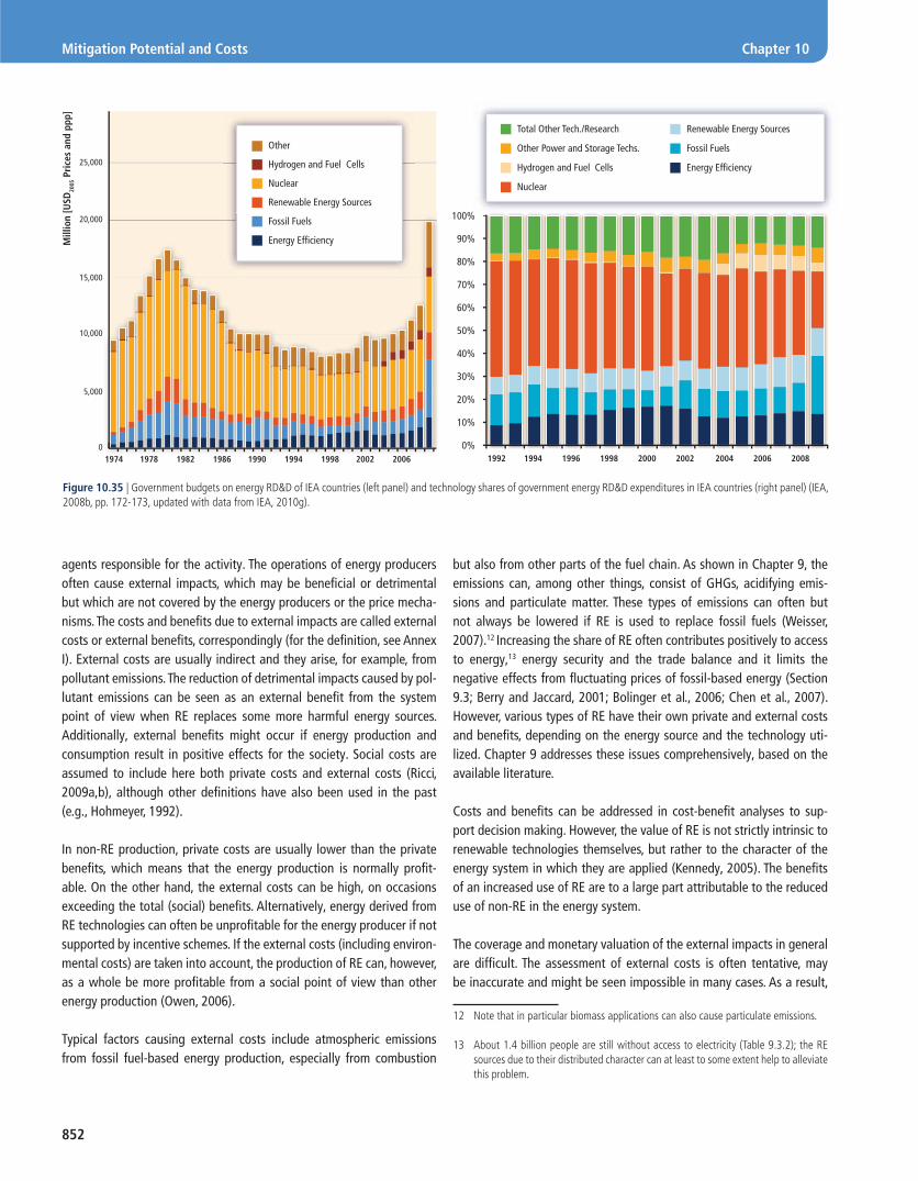
852


agents responsible for the activity. The operations of energy producers often cause external impacts, which may be benefi cial or detrimental but which are not covered by the energy producers or the price mecha-nisms. The costs and benefi ts due to external impacts are called external costs or external benefi ts, correspondingly (for the defi nition, see Annex I). External costs are usually indirect and they arise, for example, from pollutant emissions. The reduction of detrimental impacts caused by pol-lutant emissions can be seen as an external benefi t from the system point of view when RE replaces some more harmful energy sources. Additionally, external benefi ts might occur if energy production and consumption result in positive effects for the society. Social costs are assumed to include here both private costs and external costs (Ricci, 2009a,b), although other defi nitions have also been used in the past (e.g., Hohmeyer, 1992).

In non-RE production, private costs are usually lower than the private benefi ts, which means that the energy production is normally profi t-able. On the other hand, the external costs can be high, on occasions exceeding the total (social) benefi ts. Alternatively, energy derived from RE technologies can often be unprofi table for the energy producer if not supported by incentive schemes. If the external costs (including environ-mental costs) are taken into account, the production of RE can, however, as a whole be more profi table from a social point of view than other energy production (Owen, 2006).

Typical factors causing external costs include atmospheric emissions from fossil fuel-based energy production, especially from combustion

but also from other parts of the fuel chain. As shown in Chapter 9, the emissions can, among other things, consist of GHGs, acidifying emis-sions and particulate matter. These types of emissions can often but not always be lowered if RE is used to replace fossil fuels (Weisser, 2007).12 Increasing the share of RE often contributes positively to access to energy,13 energy security and the trade balance and it limits the negative effects from fl uctuating prices of fossil-based energy (Section 9.3; Berry and Jaccard, 2001; Bolinger et al., 2006; Chen et al., 2007). However, various types of RE have their own private and external costs and benefi ts, depending on the energy source and the technology uti-lized. Chapter 9 addresses these issues comprehensively, based on the available literature.

Costs and benefi ts can be addressed in cost-benefi t analyses to sup-port decision making. However, the value of RE is not strictly intrinsic to renewable technologies themselves, but rather to the character of the energy system in which they are applied (Kennedy, 2005). The benefi ts of an increased use of RE are to a large part attributable to the reduced use of non-RE in the energy system.

The coverage and monetary valuation of the external impacts in general are diffi cult. The assessment of external costs is often tentative, may be inaccurate and might be seen impossible in many cases. As a result,

12 Note that in particular biomass applications can also cause particulate emissions.

13 About 1.4 billion people are still without access to electricity (Table 9.3.2); the RE sources due to their distributed character can at least to some extent help to alleviate this problem.

Figure 10.35 | Government budgets on energy RD&D of IEA countries (left panel) and technology shares of government energy RD&D expenditures in IEA countries (right panel) (IEA, 2008b, pp. 172-173, updated with data from IEA, 2010g).

0

5,000

10,000

15,000

25,000

20,000

Other

Hydrogen and Fuel Cells

Nuclear

Renewable Energy Sources

Fossil Fuels

Energy Efficiency

0%

10%

20%

30%

40%

50%

60%

70%

80%

90%

100%

Total Other Tech./Research

Other Power and Storage Techs.

Hydrogen and Fuel Cells

Nuclear

Renewable Energy Sources

Fossil Fuels

Energy Efficiency

Mill

ion

[USD

2005

Pri

ces

and

ppp]

200620021998199419901974 1978 1982 1986 200820062004200220001998199619941992

853


the cost-benefi t analysis of some measure or policy, where the benefi t arises from decreases in an environmental or external impact, is often contentious. In contrast, the difference between benefi ts and costs can be made clear even though the concrete numbers of the cost and ben-efi t terms are uncertain. The long time spans associated with climate change and its impacts are not easy to consider in cost-benefi t analy-ses. Discounting of impacts over long time horizons is at least to some extent problematic (Weitzman, 2007; Dietz and Stern, 2008). Further, many environmental impacts are not well understood or highly complex and their consideration and monetary valuation is diffi cult. Moreover, there are usually no compensation mechanisms that could balance costs and benefi ts among different stakeholders (Soderholm and Sundqvist, 2003). These aspects might limit the use of cost-benefi t analysis and require other approaches, such as public consultation and direct setting of environmental targets and cost-benefi t or cost-effectiveness analy-ses under these targets (Krewitt, 2002; Soderholm and Sundqvist, 2003; Grubb and Newbery, 2008).

Against this background, the objective of this section is to synthesize and discuss external costs and benefi ts of increased RE use in relation to climate change mitigation. The results are presented by technology at global and regional levels. Therefore, the section defi nes the cost cat-egories considered and identifi es quantitative estimates or qualitative assessments for costs by category type, by RE type, and as far as possible also by geographical area.

This section has links to the other chapters of this report, such as Chapters 1 and 9. Parts of this section consider the same topics, but from the viewpoints of external costs and benefi ts. The external costs and benefi ts considered in this section complement the cost considerations in the other parts of the chapter, forming a more holistic picture of costs from the social viewpoint.

10.6.2 Review of studies on external costs and benefi ts

Energy extraction, conversion and use cause signifi cant environmental impacts and social costs. Many environmental impacts can be lowered by reducing emissions with advanced emission control technologies (Amann, 2008).

Although replacing fossil fuel-based energy with RE can reduce GHG emissions and also to some extent other environmental impacts and social costs caused by them, RE can also have environmental impacts and external costs, depending on the energy source and technology (da Costa et al., 2007). These impacts and costs should be lowered and of course should be considered if a comprehensive cost assessment is required.

This section considers studies in a cost and benefi t category and pres-ents a summary regarding energy sources as well. Some of the studies are global in nature, and to some extent regional studies, mostly for Europe and North America, will also be quoted. The number of studies for other regions is still limited. Many studies consider only one energy source or technology, but some studies cover a wider list of energy sources and technologies.

In the case of energy production technologies based on combustion, the impacts and external costs, in particular the environmental costs, mainly arise from emissions to air, especially if the greenhouse impact and health impact are considered. The lifecycle approach, including impacts via all stages of the energy production chain, is, however, necessary in order to recognize and account for total impact (Section 9.3.4). This holds true also in the case of non-combustible energy sources (WEC, 2004a; Kirkinen et al., 2008; Ricci, 2009a,b).

10.6.2.1 Climate change

The damage due to changing climate is often described by linking CO2 emissions with the social costs of their impacts. This relation is called social costs of carbon (SCC), which is expressed as social costs per tonne of carbon or CO2 released. A number of studies have been published on this subject and on the use of SCC in decision making (e.g., Anthoff, 2007; Grubb and Newbery, 2008; Watkiss and Downing, 2008).

The monetary evaluation of the impacts of the changing climate is diffi -cult, however. To a large extent, the impacts manifest themselves slowly over a long period of time. In addition, the impacts can arise very far from a polluter in ecosystems and societies that are very different from the ecosystems and the society found at the polluter’s location. It is for this reason that, for example, the methods used by the Stern (2007) review for damage cost accounting on a global scale are criticized, but they can also be seen as a choice for producing reasonable qualitative estimates. Apart from the question about discount rate, which is quite relevant considering the long term impacts of GHG emissions, consider-able uncertainty exists in areas such as climate sensitivity, damages due to climate change, valuation of damages and equity weighting (Watkiss and Downing, 2008).

A German study (Krewitt and Schlomann, 2006) addressing external costs uses the values of USD 17/t CO2, USD 90/t CO2 and USD 350/t CO2 (€ 14,70 and 280/t CO2 ) for the lower limit, best guess and upper limit for SCC, respectively, referring to Downing et al. (2005) and Watkiss and Downing (2008). The study assesses that the range of the esti-mated SCC values covers three orders of magnitude, which can be explained by the many different choices possible in modelling and

854


approaches to quantifying the damages. As a benchmark lower limit for global decision making, they give a value of about USD2005 17/t CO2 (£35/t CO2 ). They do not give any best guess or upper limit benchmark value, but recommend that further studies should be done on the basis of long-term climate change mitigation stabilization levels.

The price of carbon can also be considered from other standpoints, for example, what price level of CO2 emissions is needed in order to limit the atmospheric concentration to a given stabilization level. Emission trading gives also a price for carbon that is linked to the total allotted amount of emissions. Another way is to see the SCC as insurance for reducing the risks of climate change (Grubb and Newbery, 2008).

RE sources have usually quite low GHG emissions per each energy unit produced (see Chapter 9.3; WEC, 2004a; IPCC, 2007; Krewitt, 2007), so the impacts through climate change and the external costs they cause are usually low. There can also be exceptions, for example, in some cases of fuels requiring long refi ning chains like transportation biofuels produced under unfavourable conditions (Hill et al., 2006; Soimakallio et al., 2009) or land clearing for increasing biofuel pro-duction (Edwards et al., 2008; Searchinger et al., 2008).

Increasing the use of RE sources often displaces fossil energy sources that have relatively high GHG emissions and external costs (Koljonen et al., 2008). The net impact of an increase in RE supply is therefore positive external benefi ts if the whole system is considered. The magnitude of these positive impacts will depend in large part on the properties of the original energy system (Kennedy, 2005).

10.6.2.2 Health impacts due to air pollution

Combustion of both renewable fuels and fossil fuels often causes emissions of particulates and gases that have health impacts (Section 9.3.4; Krewitt, 2002; Torfs et al., 2007; Amann, 2008; Smith et al., 2009; Committee on Health, 2010). Exposure to smoke aerosols can be excep-tionally large in primitive traditional burning of solid fuels, for example, in cooking of food in developing countries (see Section 9.3; Bailis et al., 2005). Also, emissions to the environment from stacks can reach people living far from the emission sources. The exposure and the num-ber of health impacts depend on the physical and chemical character of the particulates, their concentrations in the air and population density (Krewitt, 2007). The exposure statistically leads to increased morbidity and mortality. The relationships between exposure and health impacts are estimated on the basis of epidemiological studies (e.g., Torfs et al., 2007). The external costs of increased mortality can be assessed using, for example, the concepts of value of life years lost (Preiss, 2009; Ricci, 2010) or value of statistical life (Committee on Health, 2010).

The results depend on many assumptions in the modelling, calcula-tions and epidemiological studies. Krewitt (2002) describes how the

estimated external costs of fossil-based electricity production have changed by a factor of ten during the ExternE project period between the years 1992 and 2002. ExternE is a major research programme launched by the European Commission at the beginning of the 1990s to provide a scientifi c basis for the quantifi cation of energy-related externalities. The cost estimates have been increased by extension of the considered area (more people affected) and by inclusion of the chronic mortality. Furthermore, the cost estimates have been lowered by changing the indicator for costs arising from deaths and by using new exposure-impact models. It can be argued that the results include considerable uncertainty (Torfs et al., 2007).

The typical specifi c external costs through various impact chains per tonne of emissions have been assessed, for example, in Krewitt and Schlomann (2006), Preiss (2009) and Committee on Health (2010), to be for sulphur dioxide (SO2) about USD 4,000 to 10,000/t, for nitrous oxides (NOx) about USD2005 2,000 to 10,000/t, and for particulates PM2.5 about USD 10,000 to 30,000/t. The wide ranges of values give a picture of variability and uncertainty.

When RE is used to replace fossil energy, the total social costs of the total energy system due to health impacts usually decrease (Kennedy, 2005; Bollen et al., 2009), which can be interpreted to lead to social benefi ts linked to the increase of RE. However, this is not always the case, as discussed in this section, but requires a more detailed analysis.

10.6.2.3 Other impacts

RE can have impacts on waters, land use, soil, ecosystems and biodi-versity (Section 9.3.4). It can also have a positive infl uence on energy security and trade balance and rural employment or have impacts on other socioeconomic aspects. Some of these impacts are not in a strict sense external as they are covered by price mechanisms, although they can be of importance from the viewpoints of the society. Most of these impacts have been considered in the technology Chapters 2 to 7 or in Chapter 9 in detail. The external costs due to these impacts are usu-ally lower than the external costs due to GHG emissions or due to health effects caused by pollutant emissions (Krewitt and Schlomann, 2006; Preiss, 2009; Committee on Health, 2010; Ricci, 2010). However, in some cases specifi c impacts may cause considerable external costs that should be evaluated on the project by project basis. Some informa-tion on the magnitudes of the impacts can be found in Section 10.6.3.

10.6.3 Social and environmental costs and benefi ts by energy sources and regional considerations

Most of the studies covered in this section consider North America (Gallagher et al., 2003; Roth and Ambs, 2004; Kennedy, 2005; Chen et al., 2007; Committee on Health, 2010; Kusiima and Powers, 2010)

855


Table 10.11 | External costs (US cents/kWh (3,600 kJ)) due to electricity production based on RE sources and fossil energy in Central European conditions. Valuation of climate change is based on an SCC value of 90 USD/t CO2 (Krewitt and Schlomann, 2006). Uncertainty ranges are not reported in the table. For uncertainty estimates, see Figure 10.36.

PV (2000)

PV (2030)

Hydro 300 kW

Wind 1.5 MW Onshore

Wind 2.5 MW Offshore

Geo-thermal

SolarThermal

Ligniteη=40%

Lignite Comb.Cη=48%

Coalη=43%

Coal Comp.Cη=46%

Natural Gas

η=58%

Climate change 0.86 0.48 0.11 0.09 0.08 0.33 0.11 9.3 8.0 7.4 6.9 3.4

Health 0.43 0.25 0.075 0.09 0.04 0.15 0.11 0.63 0.35 0.46 0.33 0.21

Ecosystems • • • • • • • • • • • •

Material damages

0.011 0.008 0.001 0.001 0.001 0.004 0.002 0.019 0.010 0.016 0.01 0.006

Agricultural losses

0.006 0.004 0.001 0.002 0.0005 0.002 0.001 0.013 0.005 0.011 0.006 0.005

Large accidents • • • • • • • • • • • •

Proliferation • • • • • • • • • • • •

Energy security • • • • • • • • • • • •

Geo-political effects • • • • • • • • • • • •

Sum ~1.3 ~0.74 ~0.19 ~0.18 ~0.12 ~0.49 ~0.22 >9.9 >8.4 >7.9 >7.2 >3.6

Notes: • ‘green light’: no signifi cant impacts or external costs worth mentioning (Krewitt and Schlomann, 2006). • ‘yellow’: impacts will arise that cannot be neglected and that will cause external costs. Comb.C: combined gas turbine and steam cycles; η: effi ciency factor.

and Europe (Groscurth et al., 2000; Bergmann et al., 2006; Krewitt and Schlomann, 2006; Ricci, 2009b), whilst some are more general without a specifi c geographical area.

Some studies consider developing countries. Da Costa et al. (2007) dis-cuss social features of energy production and use in Brazil. Fearnside (1999, 2005) and Oliveira and Rosa (2003) studied large hydropower projects and the technical potential of wastes in Brazil, respectively. Sparovek et al. (2009) investigated the impacts of the extension of sug-arcane production in Brazil. Bailis et al. (2005) considered biomass- and petroleum-based domestic energy scenarios in Africa and their impacts on mortality on the basis of particulate emissions. Spalding-Fecher and Matibe (2003) studied total external costs of coal-fi red power genera-tion in South Africa. Amann (2008) studied cost-effective reduction of emissions of air pollutants and GHGs in China.

Studies concerning different areas of the globe are still sparse. More investigations, articles and reports are needed to provide information on external costs and their possible variation in the ecosystems and societies of different geographical areas.

To calculate the net impact in terms of social costs of an extension of RE sources, two things have to be done. First, (a) the external costs and benefi ts can be assessed on the basis of the lifecycle approach for each technology in the conditions typical for that technology so that only

the direct impacts of that technology are taken into account (Pingoud et al., 1999; Roth and Ambs, 2004; Krewitt and Schlomann, 2006; Ricci, 2009b). The other thing (b) is to consider the RE technologies as parts of the total energy system and society, when the impacts of a possible increase in the use of the RE technologies can be assessed as causing decreases in the use and external costs of other energy sources. These decreases in external costs can be seen as external benefi ts of the RE technologies for society (Kennedy, 2005; Loulou et al., 2005; Koljonen et al., 2009).

An assessment of external costs in Central European conditions is presented in Table 10.11 (Krewitt and Schlomann, 2006). It can be seen that the social costs due to climate change and health impacts dominate the results in Table 10.11. The other impacts make a lesser contribution to the fi nal results, keeping in mind that not all impacts are quantifi able. Even if the low-end SCC value of USD 17/t CO2 assumed in the reference is used in Table 10.11 instead of USD 90/t CO2, the climate impact still dominates in the total social costs of fossil-based technologies, but for renewable technologies the health impacts would be dominant.

Figure 10.36 shows the large uncertainty ranges of two dominant external cost components, namely climate- and health-related external costs. As one example, a recent extensive study made for the condi-tions in the USA (Committee on Health, 2010) arrived at almost similar

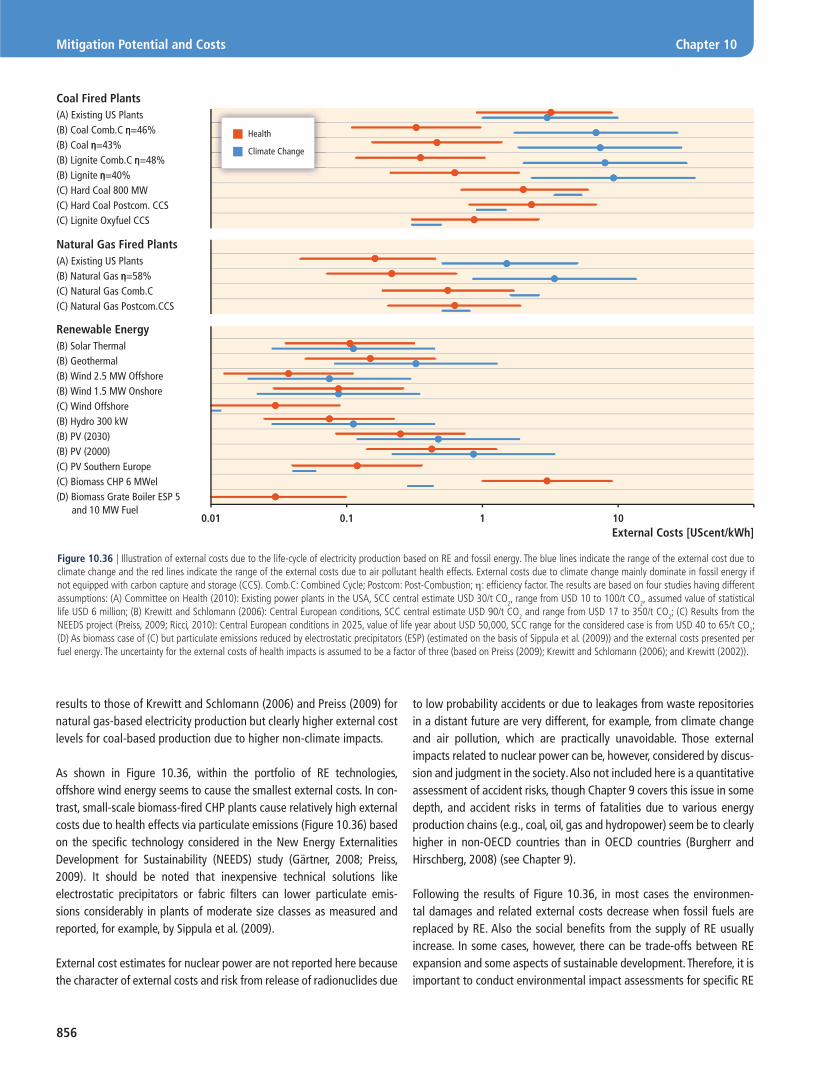
856


results to those of Krewitt and Schlomann (2006) and Preiss (2009) for natural gas-based electricity production but clearly higher external cost levels for coal-based production due to higher non-climate impacts.

As shown in Figure 10.36, within the portfolio of RE technologies, offshore wind energy seems to cause the smallest external costs. In con-trast, small-scale biomass-fi red CHP plants cause relatively high external costs due to health effects via particulate emissions (Figure 10.36) based on the specifi c technology considered in the New Energy Externalities Development for Sustainability (NEEDS) study (Gärtner, 2008; Preiss, 2009). It should be noted that inexpensive technical solutions like electrostatic precipitators or fabric fi lters can lower particulate emis-sions considerably in plants of moderate size classes as measured and reported, for example, by Sippula et al. (2009).

External cost estimates for nuclear power are not reported here because the character of external costs and risk from release of radionuclides due

to low probability accidents or due to leakages from waste repositories in a distant future are very different, for example, from climate change and air pollution, which are practically unavoidable. Those external impacts related to nuclear power can be, however, considered by discus-sion and judgment in the society. Also not included here is a quantitative assessment of accident risks, though Chapter 9 covers this issue in some depth, and accident risks in terms of fatalities due to various energy production chains (e.g., coal, oil, gas and hydropower) seem be to clearly higher in non-OECD countries than in OECD countries (Burgherr and Hirschberg, 2008) (see Chapter 9).

Following the results of Figure 10.36, in most cases the environmen-tal damages and related external costs decrease when fossil fuels are replaced by RE. Also the social benefi ts from the supply of RE usually increase. In some cases, however, there can be trade-offs between RE expansion and some aspects of sustainable development. Therefore, it is important to conduct environmental impact assessments for specifi c RE

Health

Climate Change

Renewable Energy(B) Solar Thermal(B) Geothermal(B) Wind 2.5 MW Offshore(B) Wind 1.5 MW Onshore(C) Wind Offshore(B) Hydro 300 kW(B) PV (2030) (B) PV (2000) (C) PV Southern Europe(C) Biomass CHP 6 MWel (D) Biomass Grate Boiler ESP 5 and 10 MW Fuel

0.01 0.1 1 10External Costs [UScent/kWh]

Coal Fired Plants(A) Existing US Plants(B) Coal Comb.C n=46%(B) Coal n=43%(B) Lignite Comb.C n=48%(B) Lignite n=40%(C) Hard Coal 800 MW(C) Hard Coal Postcom. CCS(C) Lignite Oxyfuel CCS

Natural Gas Fired Plants(A) Existing US Plants(B) Natural Gas n=58%(C) Natural Gas Comb.C(C) Natural Gas Postcom.CCS

Figure 10.36 | Illustration of external costs due to the life-cycle of electricity production based on RE and fossil energy. The blue lines indicate the range of the external cost due to climate change and the red lines indicate the range of the external costs due to air pollutant health effects. External costs due to climate change mainly dominate in fossil energy if not equipped with carbon capture and storage (CCS). Comb.C: Combined Cycle; Postcom: Post-Combustion; η: effi ciency factor. The results are based on four studies having different assumptions: (A) Committee on Health (2010): Existing power plants in the USA, SCC central estimate USD 30/t CO2, range from USD 10 to 100/t CO2, assumed value of statistical life USD 6 million; (B) Krewitt and Schlomann (2006): Central European conditions, SCC central estimate USD 90/t CO2 and range from USD 17 to 350/t CO2; (C) Results from the NEEDS project (Preiss, 2009; Ricci, 2010): Central European conditions in 2025, value of life year about USD 50,000, SCC range for the considered case is from USD 40 to 65/t CO2; (D) As biomass case of (C) but particulate emissions reduced by electrostatic precipitators (ESP) (estimated on the basis of Sippula et al. (2009)) and the external costs presented per fuel energy. The uncertainty for the external costs of health impacts is assumed to be a factor of three (based on Preiss (2009); Krewitt and Schlomann (2006); and Krewitt (2002)).

857


Tem

pera

ture

Ris

e

Reduction of Local Air Pollutants

Mitigation of Climate Change

Costs of Measures

Hea

lth

Effe

cts

[PM

Dea

ths]

Incr

ease

d W

elfa

re[D

isco

unte

d Co

nsum

ptio

n %

of B

asel

ine]

Mitigation of Climate

Change Only

Base Line Reduction of Local Air

Pollutants Only

Combined Strategyof Mitigation ofClimate Changeand Reduction of

Air Pollutants

5°C

1,000

2%

1,080

850

63 66

3,0ºC

4,7ºC

3,3ºC

4,8ºC

1,51,7

Figure 10.37 | Illustration of changes in costs, benefi ts and global welfare for three scenarios (‘reduction of local air pollutants’, ‘mitigation of climate change’, and ‘combined strategy of mitigation of climate change and reduction of local air pollutants’), expressed as percentage consumption change (welfare increase) in comparison to the baseline (lower panel). The global temperature rise (degrees Celsius compared to the pre-industrial level) and number of deaths due to air pollution (millions) are given in the upper panel for each scenario. In the scenario ‘mitigation of climate change only’, the external costs of climate change have been internalized; in the scenario ‘reduction of local air pollutants only’, the external costs of local air pollutants have been internalized; and in the scenario of ‘combined strategy’, both external cost components have been internalized. The ‘com-bined strategy’ is most benefi cial for society according to the results. In the baseline, the number of particulate matter (PM) deaths due to air pollutants would be around 1,000 million and the temperature rise 4.8°C (Bollen et al., 2009).


Considerable uncertainties exist in the assessment and valuation of external impacts of energy sources. The assessment of physical, bio-logical and health damages includes considerable uncertainty and the estimates are based typically on purely quantitative models, the results of which are often diffi cult to validate. The damages or changes seldom have market values that could be used in cost esti-mation, thus indirect information or other approaches must be used for damage valuation. Further, many of the damages will take place far in the future or in societies very different from those benefi ting from the use of the considered energy production, which complicates the considerations. These factors contribute to the uncertainty about external costs.

However, the knowledge about external costs and benefi ts due to alternative energy sources can give some guidance for society to select best alternatives and to steer the energy system towards over-all effi ciency and high welfare gains.

projects under consideration in order to be sure that essential requirements for the implementation of the projects are realized. Chapter 9 discusses this topic in more detail.

Figure 10.36 can only summarize a part of the available literature. Some additional studies have, for example, considered the external costs from alternative transportation biofuels and other energy sources for automobiles (Hill et al., 2006, 2009; Committee on Health, 2010). The results suggest that lower external costs per vehicle kilometre than from fossil fuels can be achieved in many cases by using biofuels, but not always. Case-specifi c studies are needed to assess the impacts of con-sidered feedstock cultivation and harvest, as well as fuel processing and use.

10.6.4 Synergistic strategies for limiting damages and external costs

Many environmental impacts and external costs follow from the use of energy sources and energy technologies that cause GHG emissions, par-ticulate emissions and acidifying emissions—fossil fuel combustion being a prime example. Therefore, it might be benefi cial to consider the reduction of emission-related impacts using integrated strategies (Amann, 2008; Bollen et al., 2009).

Bollen et al. (2009) have made global cost-benefi t studies using the MERGE model (Manne and Richels, 2005). In their studies, the external costs of health effects due to particulate emissions and impacts of climate change were internalized. According to the study (Figure 10.37), the external benefi ts were greatest when both external cost types were internalized, although the miti-gation costs were high as they work in a shorter time frame. The discounted benefi ts from the control of particulate emissions are clearly larger than the discounted benefi ts from the mitigation of climate change. The difference is, according to a sensitivity study, mostly greater by at least a factor of two, but of course depends on the specifi c assumptions. The countries would therefore benefi t from combined strategies quite rapidly due to decreased external costs stemming from the reduced air pollution health impacts.

Amann (2008) reached quite similar conclusions in a case study for China. According to the study, the reduction of GHG emissions in China caused considerable benefi ts when there is a desire to reduce local air pollution. Also a study (Syri et al., 2002) considering the impacts of the reduction of GHG emissions in Finland stated that particulate emissions are also likely to decrease.

A study by Spalding-Fecher and Matibe (2003) is one of the few for devel-oping countries. They found that, in South Africa, the total external costs of coal-fi red power generation are 40 and 20% of industrial and residential charges for electricity. They concluded also that a reduction in GHG emis-sions lessens air-borne particulates that led to respiratory disorders and other diseases.

858


References

Aitken, D. (2003). Transitioning to a Renewable Energy Future. White Paper,

International Solar Energy Society, Freiburg, Germany, 55 pp. Available at: www.

ises.org/shortcut.nsf/to/wp.

Akimoto, K., F. Sano, J. Oda, T. Homma, U.K. Rout, and T. Tomoda (2008). Global

emission reductions through a sectoral intensity target scheme. Climate Policy,

8(Supplement), pp. S46-S59.

Amann, M. (2008). GAINS ASIA Scenarios for Cost-Effective Control of Air Pollution

and Greenhouse Gases in China. International Institute for Applied Systems

Analysis, Laxenburg, Austria

Anthoff, D. (2007). Marginal external damage costs inventory of greenhouse gas

emissions. Delivery No. 5.4 - RS 1b, New Energy Externalities Developments for

Sustainability, Rome, Italy.

Awerbuch, S. (2006). Portfolio-based electricity generation planning: Policy implica-

tions for renewables and energy security. Mitigation and Adaptation Strategies

for Global Change, 11(3), pp. 693-710.

Azar, C., K. Lindgren, E. Larson, and K. Möllersten (2006). Carbon capture and

storage from fossil fuels and biomass – Costs and potential role in stabilizing the

atmosphere. Climatic Change, 74(1), pp. 47-79.

Bailis, R., M. Ezzati, and D.M. Kammen (2005). Mortality and greenhouse gas

impacts of biomass and petroleum energy futures in Africa. Science, 308(5718),

pp. 98-103.

Baker, E., L. Clarke, and E. Shittu (2008). Technical change and the marginal cost

of abatement. Energy Economics, 30(6), pp. 2799-2816.

Barker, T., I. Bashmakov, A. Alharthi, M. Amann, L. Cifuentes, J. Drexhage,

M. Duan, O. Edenhofer, B. Flannery, M. Grubb, M. Hoogwijk, F.I. Ibitoye,

C.J. Jepma, W.A. Pizer, and K. Yamaji (2007). Mitigation from a cross-sectoral

perspective. In: Climate Change 2007: Mitigation of Climate Change. Contribution

of Working Group III to the Fourth Assessment Report of the Intergovernmental

Panel on Climate Change. B. Metz, O.R. Davidson, P.R. Bosch, R. Dave, and L.A.

Meyer (eds.), Cambridge University Press, pp. 619-690.

Barker, T., H. Pun, J. Köhler, R. Warren, and S. Winne (2006). Decarbonizing the

global economy with induced technological change: Scenarios to 2100 using

E3MG. Energy Journal, 27(Special Issue 1), pp. 241-258.

Bergmann, A., M. Hanley, and R. Wright (2006). Valuing the attributes of renew-

able energy investments. Energy Policy, 34(9), pp. 1004-1014.

Berry, T., and M. Jaccard (2001). The renewable portfolio standard: design consider-

ations and an implementation survey. Energy Policy, 29(4), pp. 263-277.

Black & Veatch Corporation (2007). Arizona Renewable Energy Assessment. Final

Report. Black & Veatch Corporation, Lamar, Kansas.

Bolinger, M., R. Wiser, and W. Golove (2006). Accounting for fuel price risk when

comparing renewable to gas-fi red generation: the role of forward natural gas

prices. Energy Policy, 34(6), pp. 706-720.

Bollen, J., B. van der Zwaan, C. Brink, and H. Erens (2009). Local air pollution and

global climate change: A combined cost-benefi t analysis. Resource and Energy

Economics, 31, pp. 161-181.

Bosetti, V., C. Carraro, and M. Tavoni (2009). Climate change mitigation strate-

gies in fast-growing countries: The benefi ts of early action. Energy Economics,

31(Supplement 2), pp. S144-S151.

Burgherr, P., and S. Hirschberg (2008). A comparative analysis of accident risks in

fossil, hydro and nuclear energy chains. Human and Ecological Risk Assessment,

14, pp. 947-973.

Calvin, K., J. Edmonds, B. Bond-Lamberty, L. Clarke, S.H. Kim, P. Kyle, S.J. Smith,

A. Thomson, and M. Wise (2009). 2.6: Limiting climate change to 450 ppm

CO2 equivalent in the 21st century. Energy Economics, 31(Supplement 2), pp.

S107-S120.

Carlsmith, R.S., W.U. Chandler, J.E. McMahon, and D.J. Santini (1990). Energy

Effi ciency: How Far can We Go? ORNL/TM-11441, Oak Ridge National Laboratory,

Oak Ridge, TN, USA, 83 pp.

Carpenter, S.R., P.L. Pingali, E.M. Bennet, and M.B. Zurek (eds.) (2005).

Ecosystems and Human Wellbeing: Scenarios. Island Press, Chicago, IL, USA,

561 pp.

CBI (2007). Climate Change: Everyone’s Business. Confederation of British Industry

Climate Change Task Force, London, UK.

Changliang, X., and S. Zhanfeng (2009). Wind energy in China: Current scenario

and future perspectives. Renewable and Sustainable Energy Reviews, 13(8), pp.

1966-1974.

Chen, W. (2005). The Costs of Mitigating Carbon Emissions in China: Findings from

China MARKALMACRO modeling. Energy Policy, 33, pp. 885-896.

Chen, C., R. Wiser, and M. Bolinger (2007). Weighing the Costs and Benefi ts of

State Renewables Portfolio Standards: A Comparative Analysis of State-Level

Policy Impact Projections. LBNL-61580, Ernest Orlando Lawrence Berkeley

National Laboratory, Berkeley, CA, USA, 71 pp.

Clarke, L., J. Edmonds, H. Jacoby, H. Pitcher, J. Reilly, and R. Richels (2007).

Scenarios of Greenhouse Gas Emissions and Atmospheric Concentrations. Sub-

report 2.1A of Synthesis and Assessment Product 2.1. U.S. Department of Energy,

Offi ce of Biological and Environmental Research, Washington, DC, USA, 154 pp.

Clarke, L., J.P. Weyant, and J. Edmonds (2008). On the sources of technological

change: what do the models assume. Energy Economics, 30(2), pp. 409-424.

Clarke, L., J. Edmonds, V. Krey, R. Richels, S. Rose, and M. Tavoni (2009).

International climate policy architectures: Overview of the EMF 22 International

Scenarios. Energy Economics, 31(Supplement 2), pp. 64-81.

Committee on Climate Change (2008). Building a Low-Carbon Economy – The

UK’s Contribution to Tackling Climate Change. The Stationary Offi ce, Norwich,

UK. Available at: www.theccc.org.uk/reports/building-a-low-carbon-economy.

Committee on Health (2010). Hidden Costs of Energy: Unpriced Consequences of

Energy Production and Use. Committee on Health, Environmental, and Other

External Costs and Benefi ts of Energy Production and Consumption, National

Research Council, National Academies Press, Atlanta, GA, USA, 506 pp.

Creyts, J., A. Derkach, S. Nyquist, K. Ostrowski, and J. Stephenson (2007).

Reducing U.S. Greenhouse Gas Emissions: How Much at What Cost? McKinsey

& Company, USA, 83 pp.

Curtright, A.E., M.G. Morgan, and D.W. Keith (2008). Expert assessments of

future photovoltaic technologies. Environmental Science & Technology, 42(24),

pp. 9031-9038.

da Costa, M.M., C. Cohen, and R. Schaeffer (2007). Social features of energy

production and use in Brazil: Goals for a sustainable energy future. Natural

Resources Forum, 31(1), pp. 11-20.

Dasgupta, P., K.-G. Mäler, and S. Barrett (2000). Intergenerational Equity, Social

Discount Rates and Global Warming. University of Cambridge, Cambridge, UK.

859


de Vries, B.J.M., D.P. van Vuuren, and M.M. Hoogwijk (2007). Renewable energy

sources: Their global potential for the fi rst-half of the 21st century at a global

level: An integrated approach. Energy Policy, 35, pp. 2590-2610.

den Elzen, M., N. Höhne, and J. van Vliet (2009). Analysing comparable greenhouse

gas mitigation efforts for Annex I countries. Energy Policy, 37, pp. 4114-4131.

Dietz, S., and N. Stern (2008). Why economic analysis supports strong action on

climate change: A response to the Stern review’s critics. Review of Environmental

Economics and Policy, 2(1), pp. 94-113.

Dornburg, V., J. van Dam, and A. Faaij (2007). Estimating GHG emission mitiga-

tion supply curves of large-scale biomass use on a country level. Biomass and

Bioenergy, 31(1), pp. 46-65.

Downing, T., D. Anthoff, R. Butterfi eld, M. Ceronsky, M. Grubb, J. Guo,

C. Hepburn, C. Hope, A. Hunt, A. Li, A. Markandya, S. Moss, A. Nyong, R. Tol, and

P. Watkiss (2005). Social Cost of Carbon: A Closer Look at Uncertainty. Stockholm

Environment Institute, Oxford, UK.

Durstewitz, M., and M. Hoppe-Klipper (1999). Wind energy experience curve

for the German “250 MW Wind Program”. In: IEA International Workshop on

Experience Curves for Policy Making - The Case of Energy Technologies. Stuttgart,

Germany, 10-11 May 1999. Available at: www.iset.uni-kassel.de/abt/FB-I/publi-

cation/99-05-10_exp_curves_iea.pdf.

ECN (2004). Learning from the Sun: Final Report of the Photes Project. Energy

Research Center of the Netherlands (ECN), Petten, The Netherlands.

Edenhofer, O., C. Carraro, J. Köhler, and M. Grubb (guest eds.) (2006).

Endogenous technological change and the economics of atmospheric stabiliza-

tion. Energy Journal, 27(Special Issue 1), 284 pp.

Edenhofer, O., C. Carraro, J.-C. Hourcade, K. Neuhoff, G. Luderer, C. Flachsland,

M. Jakob, A. Popp, J. Steckel, J. Strohschein, N. Bauer, S. Brunner,

M. Leimbach, H. Lotze-Campen, V. Bosetti, E.d. Cian, M. Tavoni, O. Sassi,

H. Waisman, R. Crassous-Doerfl er, S. Monjon, S. Dröge, H.v. Essen, P.d. Río,

and A. Türk (2009). The Economics of Decarbonization – Report of the RECIPE

Project. Potsdam Institute for Climate Impact Research, Potsdam, Germany.

Edenhofer, O., B. Knopf, T. Barker, L. Baumstark, E. Bellevrat, B. Chateau,

P. Criqui, M. Isaac, A. Kitous, S. Kypreos, M. Leimbach, K. Lessmann, B. Magne,

Å. Scrieciu, H. Turton, and D.P. Van Vuuren (2010). The economics of low sta-

bilization: Model comparison of mitigation strategies and costs. Energy Journal,

31(Special Issue), pp. 11-48.

Edwards, R., S. Szekeres, F. Neuwahl, and V. Mahieu (2008). Biofuels in the

European Context: Facts, Uncertainties and Recommendations. JRC Institute for

Energy, Petten, The Netherlands, 30 pp.

EEA (2007). Greenhouse gas emission trends and projections in Europe 2007 –

Country profi le: Poland. European Energy Agency, Brussels, Belgium.

EEA (2009). Europe’s onshore and offshore wind energy potential: An assessment

of environmental and economic constraints. European Environment Agency,

Copenhagen, Denmark.

EIA (2009). Annual Energy Outlook 2009 with Projections to 2030. Energy

Information Administration, Washington, DC, USA.

Enermodal (1999). Cost Reduction Study for Solar Thermal Power Plants: Final

Report. Enermodal Engeneering Limited, Kitchener, ON, Canada.

Enviros Consulting Ltd. (2005). The Costs of Supplying Renewable Energy. Enviros

Consulting Ltd., London, UK.

EPIA (2008). Solar Generation. European Photovoltaic Industry Association (EPIA),

Brussels, Belgium.

EPIA (2010). Global Market Outlook for Photovoltaics until 2014. European

Photovoltaic Industry Association (EPIA), Brussels, Belgium, 8 pp.

ERI (2009). 2050 China Energy and CO2 Emissions Report (CEACER). Energy Research

Institute, Beijing: Science Press. In Chinese. As cited in: China’s Energy and Carbon

Emissions Outlook to 2050, N. Zhou and D. Fridley (2011). Lawrence Berkeley

National Laboratory.

EWEA (2009). Wind Energy, the Facts. European Wind Energy Association (EWEA),

Brussels, Belgium.

Fearnside, P.M. (1999). Social impacts of Brazil’s Tucurui Dam. Environmental

Management, 24(4), pp. 483-495.

Fearnside, P.M. (2005). Brazil’s Samuel Dam: Lessons for hydroelectric development

policy and the environment in Amazonia. Environmental Management, 35(1),

pp. 1-19.

Fellows, A. (2000). The Potential of Wind Energy to Reduce Carbon Dioxide

Emissions. Garrad Hassan, Glasgow, Scotland.

Ferioli, F., K. Schoots, and B.C.C. Van der Zwaan (2009). Use and limitations of

learning curves for energy technology policy: A component-learning hypothesis.

Energy Policy, 37, pp. 2525-2535.

Fisher, B.S., N. Nakicenovic, K. Alfsen, J. Corfee Morlot, F. de la Chesnaye,

J.-C. Hourcade, K. Jiang, M. Kainuma, E. La Rovere, A. Matysek, A. Rana,

K. Riahi, R. Richels, S. Rose, D. van Vuuren, and R. Warren (2007). Issues

related to mitigation in the long term context. In: Climate Change 2007:

Mitigation of Climate Change. Contribution of Working Group III to the Fourth

Assessment Report of the Intergovernmental Panel on Climate Change. B. Metz,

O.R. Davidson, P.R. Bosch, R. Dave, and L.A. Meyer (eds.), Cambridge University

Press, pp.169-250.

Fleiter, T., M. Hagemann, S. Hirzel, W. Eichhammer, and M. Wietschel (2009).

Costs and potentials of energy savings in European industry – a critical assess-

ment of the concept of conservation supply curves. In: Proceedings of ECEEE

2009 Summer Study, European Council for an Energy Effi cient Economy (ed.), La

Colle sur Loup, France, 1-6 June 2009, Panel 5, pp. 1261-1272. Available at: www.

eceee.org/conference_proceedings/eceee/2009/Panel_5/5.376/.

Foxon, T.J., R. Gross, A. Chase, J. Howes, A. Arnall, and D. Anderson (2005). UK

innovation systems for new and renewable energy technologies: drivers, barriers

and system failures. Energy Policy, 33, pp. 2123-2137.

Gallagher, P.W., M. Dikeman, J. Fritz, E. Wailes, W. Gauthier, and H. Shapouri

(2003). Supply and social cost estimates for biomass from crop residues in the

United States. Environmental & Resource Economics, 24(4), pp. 335-358.

Gärtner, S. (2008). Final Report on Technical Data, Costs and Life Cycle Inventories

of Biomass CHP Plants. Deliverable No. 13.2 – RS 1a, New Energy Externalities

Developments for Sustainability, Rome, Italy.

Goldemberg, J., S. Coelhob, P.M. Nastaric, and O. Lucon (2004). Ethanol learning

curve: The Brazilian experience. Biomass & Bioenergy, 26(2004), pp. 301-304.

González, P.d.R. (2008). Policy implications of potential confl icts between short-term

and long-term effi ciency in CO2 emissions abatement. Ecological Economics, 65,

pp. 292-303.

Gordon, F., L. Garth, T. Eckman, and C. Grist (2008). Beyond Energy Supply Curves.

University of California, Davis, CA, USA.

860


Groscurth, H.M., A. de Almeida, A. Bauen, F.B. Costa, S.O. Ericson, J. Giegrich,

N. von Grabczewski, D.O. Hall, O. Hohmeyer, K. Jorgensen, C. Kern, I. Kuhn,

R. Lofstedt, J.D. Mariano, P.M.G. Mariano, N.I. Meyer, P.S. Nielsen, C. Nunes,

A. Patyk, G.A. Reinhardt, F. Rosillo-Calle, I. Scrase, and B. Widmann (2000).

Total costs and benefi ts of biomass in selected regions of the European Union.

Energy, 25(11), pp. 1081-1095.

Gross, R., and P. Heptonstall (2008). The costs and the impacts of intermittency: An

ongoing debate. Energy Policy, 36(2008), pp. 4005-4007.

Grubb, M., and D. Newbery (2008). Pricing carbon for electricity generation:

national and international dimensions. In: Delivering a Low Carbon Electricity

System: Technologies, Economics and Policy. M. Grubb, T. Jamasb, and M.G. Pollitt

(eds.), Cambridge University Press.

Grubler, A. (2008). Energy transitions. In: Encyclopedia of Earth. C.J. Cleveland

(ed.), Environmental Information Coalition, National Council for Science and the

Environment, Washington, DC, USA.

Gumerman, E., J.G. Koomey, and M.A. Brown (2001). Strategies for cost-effective

carbon reductions: a sensitivity analysis of alternative scenarios. Energy Policy,

29, pp. 1313-1323.

Gurney, A., H. Ahammad, and M. Ford (2009). The economics of greenhouse gas

mitigation: Insights from illustrative global abatement scenarios modelling.

Energy Economics, 31(Supplement 2), pp. S174-S186.

Hanaoka, T., R. Kawase, M. Kainuma, Y. Matsuoka, H. Ishii, and K. Oka (2006).

Greenhouse Gas Emissions Scenarios Database and Regional Mitigation Analysis.

National Institute for Environmental Studies (NIES), Tsukuba, Japan, 106 pp.

Harmon, C. (2000). Experience Curves for Photovoltaic Technology. IR-00-014,

International Institute for Applied Systems Analysis, Laxenburg, Austria.

Heptonstall, P. (2007). A Review of Electricity Unit Cost Estimates, Working Paper.

UK Energy Research Centre, London, UK.

Herzog, H., K. Smekens, P. Dadhich, J. Dooley, Y. Fujii, O. Hohmeyer, and K. Riahi

(2005). Cost and economic potential. In: IPCC Special Report on Carbon Dioxide

Capture and Storage. B. Metz, O. Davidson, H. de Coninck, M. Loos, and L. Meyer

(eds.), Cambridge University Press, pp. 339-362.

Hettinga, W.G., H.M. Junginger, S.C. Dekker, M. Hoogwijk, A.J. McAloon, and

K.B. Hicks (2009). Understanding the reductions in US corn ethanol production

costs: An experience curve approach. Energy Policy, 37(1), pp. 190-203.

Hill, J., E. Nelson, D. Tilman, S. Polasky, and D. Tiffany (2006). Environmental,

economic, and energetic costs and benefi ts of biodiesel and ethanol biofuels.

Proceedings of the National Academy of Sciences, 103(30), pp. 11206-11210.

Hill, J., S. Polasky, E. Nelson, D. Tilman, H. Huo, L. Ludwig, J. Neumann, H. Zheng,

and D. Bonta (2009). Climate change health costs of air emissions from biofu-

els and gasoline. Proceedings of the National Academy of Sciences, 106(6), pp.

2077-2082.

Hohmeyer, O. (1992). Renewables and the full costs of energy. Energy Policy, 20(4),

pp. 365-375.

Hoogwijk, M., A. Faaij, R. van den Broek, G. Berndes, D. Gielen, and W. Turkenburg

(2003). Exploration of the ranges of the global potential of biomass for energy.

Biomass and Bioenergy, 25, pp. 119-133.

Hoogwijk, M., B. de Vries, and W. Turkenburg (2004). Assessment of the global

and regional geographical, technical and economic potential of onshore wind

energy. Energy Economics, 26, pp. 889-919.

Hoogwijk, M., and W. Graus (2008). Global Potential of Renewable Energy Sources:

A Literature Assessment. Ecofys, Utrecht, The Netherlands, 45 pp.

Hoogwijk, M., A. Faaij, B. de Vries, and W. Turkenburg (2009). Exploration of

regional and global cost-supply curves of biomass energy from short-rotation

crops at abandoned croplands and rest land under four IPCC SRES land-use sce-

narios. Biomass and Bioenergy, 33, pp. 26-43.

Hourcade, J.-C., M. Jaccard, C. Bataille, and F. Ghersi (2006). Hybrid modeling:

New answers to old challenges – Introduction to the Special Issue of The Energy

Journal. Energy Journal, 27(Special Issue October), pp. 1-12.

Hughes, A., M. Haw, H. Winkler, A. Marquard, and B. Merven (2007). Energy

Modeling: A Modelling Input into the Long Term Mitigation Scenarios Process.

LTMS Input Report. Energy Research Centre, Cape Town, South Africa.

IEA (2000). Experience Curves for Energy Technology Policy. International Energy

Agency (IEA), Paris, France, 133 pp.

IEA (2003). Energy to 2050. Scenarios for a Sustainable Future. International Energy

Agency (IEA), Paris, France.

IEA (2005). Projected Costs of Generating Electricity. OECD/IEA, Paris, France.

IEA (2006). Standard Review of the Netherlands. International Energy Agency (IEA),

Paris, France.

IEA (2007a). Renewables for Heating and Cooling, Untapped Potential. International

Energy Agency (IEA), Paris, France.

IEA (2007b). Renewables in Global Energy Supply: An IEA Fact Sheet. International


IEA (2008a). Deploying Renewable Energies: Principles for Effective Policies.

International Energy Agency (IEA), Paris, France.

IEA (2008b). Energy Technology Perspectives 2008. Scenarios and Strategies to 2050.

International Energy Agency (IEA), Paris, France, 646 pp.

IEA (2009). World Energy Outlook 2009. International Energy Agency (IEA), Paris,

France, 696 pp.

IEA (2010a). Energy Technology Perspectives 2010. Scenarios and Strategies to 2050.

International Energy Agency (IEA), Paris, France, 708 pp.

IEA (2010b). Projected Costs of Generating Electricity - 2010 Edition. International


IEA (2010c). Technology Roadmap Solar Photovoltaic Energy. International Energy

Agency (IEA), Paris, France.

IEA (2010d). World Energy Outlook 2010. International Energy Agency (IEA), Paris,

France, 736 pp.

IEA (2010e). Energy Balances of Non-OECD Countries. International Energy Agency

(IEA), Paris, France.

IEA (2010f). Key Energy Statistics 2010. International Energy Agency (IEA), Paris,

France.

IEA (2010g). RD&D Budget. IEA Energy Technology R&D Statistics (database), doi:

10.1787/data-00488-en. Available at: www.oecd-ilibrary.org/energy/data/

iea-energy-technology-r-d-statistics/rd-d-budget_data-00488-en.

IMF (2009). World Economic Outlook Update: Contractionary Forces Receding but

Weak Recovery Ahead, International Monetary Fund (IMF), Washington D.C., USA

IPCC (2000). Special Report on Emissions Scenarios. N. Nakicenovic and R. Swart

(eds.), Cambridge University Press, 570 pp.

IPCC (2007). Climate Change 2007: Mitigation of Climate Change. Contribution of

Working Group III to the Fourth Assessment Report of the Intergovernmental

Panel on Climate Change. B. Metz, O.R. Davidson, P.R. Bosch, R. Dave, and L.A.

Meyer (eds.), Cambridge University Press, 851 pp.

Isles, L. (2006). Offshore Wind Farm Development: Cost Reduction Potential. PhD

Thesis, Lund University, Lund, Sweden.

861


Jaffe, A.B., R.G. Newell, and R.N. Stavins (2005). A tale of two market failures:

Technology and environmental policy. Ecological Economics, 54(2-3), pp.

164-174.

Jamasb, T. (2007). Technical change theory and learning curves: Patterns of progress

in electricity generation technologies. Energy Journal, 28(3), pp. 133-150.

Junginger, M., S. Agterbosch, A. Faaij and W.C. Turkenburg (2004). Renewable

electricity in the Netherlands. Energy Policy, 32, pp. 1053-1073.

Junginger, M., A. Faaij, R. Björheden, and W.C. Turkenburg (2005a). Technological

learning and cost reductions in wood fuel supply chains in Sweden. Biomass and

Bioenergy, 29, pp. 399-418.

Junginger, M., A. Faaij, and W.C. Turkenburg (2005b). Global experience curves

for wind farms. Energy Policy, 33, pp. 133-150.

Junginger, M., E. Visser, K. Hjort-Gregersen, J. Koornneef, R. Raven, A. Faaij,

and W. Turkenburg (2006). Technological learning in bioenergy systems. Energy

Policy, 34, pp. 4024-4041.

Junginger, M., W.V. Sark, and A. Faaij (eds.) (2010). Technological Learning in

the Energy Sector: Lessons for Policy, Industry and Science. Edward Elgar,

Northampton, MA, USA.

Kahouli-Brahmi (2009). Testing for the presence of some features of increasing

returns to adoption factors in energy system dynamics: An analysis via the learn-

ing curve approach. Ecological Economics, 68, pp. 1195-1212.

Kennedy, S. (2005). Wind power planning: assessing long-term costs and benefi ts.

Energy Policy, 33(13), pp. 1661-1675.

Kirkinen, J., T. Palosuo, K. Holmgren, and I. Savolainen (2008). Greenhouse

impact due to the use of combustible fuels: Life cycle viewpoint and relative

radiative forcing commitment. Environmental Management, 42(3), pp. 458-469.

Kitous, A., P. Criqui, E. Bellevrat, and B. Chateau (2010). Transformation pat-

terns of the worldwide energy system – Scenarios for the century with the POLES

model. Energy Journal, 31(Special Issue), pp. 49-82.

Knopf, B., O. Edenhofer, T. Barker, N. Bauer, L. Baumstark, B. Chateau, P. Criqui,

A. Held, M. Isaac, M. Jakob, E. Jochem, A. Kitous, S. Kypreos, M. Leimbach,

B. Magne, S. Mima, W. Schade, S. Scrieciu, H. Turton, and D.v. Vuuren (2009).

The economics of low stabilisation: implications for technological change

and policy. In: Making Climate Change Work for Us: European Perspectives

on Adaptation and Mitigation Strategies. M. Hulme and H Neufeldt (eds.),

Cambridge University Press.

Koljonen, T., H. Ronde, A. Lehtilä, T. Ekholm, I. Savolainen, and S. Syri (2008).

Greenhouse gas emission mitigation and energy security, a scenario results and

practical programmes in some Asian countries. In: 2nd IAEE Asian Conference,

International Association for Energy Economics, Perth, Australia, 5-7 November

2008.

Koljonen, T., M. Flyktman, A. Lehtilä, K. Pahkala, E. Peltola, and I. Savolainen

(2009). The role of CCS and renewables in tackling climate change. Energy

Procedia, 1(1), pp. 4323-4330.

Koomey, J.G., Richey, R.C., Laitner, J.A., Markel, R.J., and Marnay, C. (1998).

Technology and Greenhouse Gas Emissions: An Integrated Analysis using the

LBNL–NEMS Model. Lawrence Berkeley National Laboratory, Berkeley, CA, USA.

Kouvaritakis, N., A. Soria, and S. Isoard (2000). Modelling energy technology

dynamics: methodology for adaptive expectations models with learning by doing

and learning by searching. International Journal of Global Issues, 14, pp. 1-4.

Krewitt, W. (2002). External costs of energy – do the answers match the questions?

Looking back at 10 years of ExternE. Energy Policy, 30(10), pp. 839-848.

Krewitt, W. (2007). Die externen Kosten der Stromerzeugung aus erneuerbaren

Energien im Vergleich zur fossilen Stromerzeugung. Umweltwissenschaften und

Schadstoff-Forschung, 19(3), pp. 144-151.

Krewitt, W., and B. Schlomann (2006). Externe Kosten der Stromerzeugung

aus erneuerbaren Energien im Vergleich zur Stromerzeugung aus fossilen

Energieträgern. DLR, Institut für Technische Thermodynamik, Fraunhofer Institut

für System-und Innovationsforschung, Gutachten im Auftrag des ZSW im Rahmen

von Beratungsleistungen für das BMU, 59 pp.

Krewitt, W., S. Teske, S. Simon, T. Pregger, W. Graus, E. Blomen, S. Schmid, and

O. Schäfer (2009). Energy [R]evolution 2008 – a sustainable world energy per-

spective. Energy Policy, 37(12), pp. 5764-5775.

Krey, V., and K. Riahi (2009). Implications of delayed participation and technol-

ogy failure for the feasibility, costs, and likelihood of staying below temperature

targets – Greenhouse gas mitigation scenarios for the 21st century. Energy

Economics, 31(Supplement 2), pp. S94-S106.

Krey, V., and L. Clarke (2011). Role of renewable energy in climate mitigation: a

synthesis of recent scenarios. Climate Policy, in press.

Kruck, C., and L. Eltrop (2007). Perspektiven der Stromerzeugung aus Solar- und

Windenergienutzung: Endbericht. FKZ A204/04, IER (Institut für Energiewirtschaft

und Rationelle Energieanwendung), Universität Stuttgart, Stuttgart, Germany.

Kuik, O., L. Brander, and R.S.J. Tol (2009). Marginal abatement costs of greenhouse

gas emissions: A meta-analysis. Energy Policy, 37, pp. 1395-1403.

Kurosawa, A. (2006). Multigas mitigation: An economic analysis using GRAPE

model. Energy Journal, 27(Special Issue November), pp. 275-288.

Kusiima, J.M., and S.E. Powers (2010). Monetary value of the environmental and

health externalities associated with production of ethanol from biomass feed-

stocks. Energy Policy, 38(6), pp. 2785-2796.

Kverndokk, S., and K.E. Rosendahl (2007). Climate policies and learning by doing:

Impacts and timing of technology subsidies. Resource and Energy Economics,

29(6), pp. 2785-2796.

Leimbach, M., N. Bauer, L. Baumstark, M. Lüken, and O. Edenhofer (2010).

Technological change and international trade – Insights from REMIND-R. Energy

Journal, 31(Special Issue), pp. 109-136.

Lewandowski, I., J. Weger, A. van Hooijdonk, K. Havlickova, J. van Dam, and

A. Faaij (2006). The potential biomass for energy production in the Czech

Republic. Biomass and Bioenergy, 30, pp. 405-421.

Loulou, R., U. Remme, A. Kanudia, A. Lehtila, and G. Goldstein (2005).

Documentation for the TIMES Model. IEA Energy Technology Systems Analysis

Programme, Paris, France.

Loulou, R., M. Labriet, and A. Kanudia (2009). Deterministic and stochastic

analysis of alternative climate targets under differentiated cooperation regimes.

Energy Economics, 31(Supplement 2), pp. S131-S143.

Luderer, G., V. Bosetti, J. Steckel, H. Waisman, N. Bauer, E. Decian, M. Leimbach,

O. Sassi, and M. Tavoni (2009). The Economics of Decarbonization – Results

from the RECIPE model Intercomparison. Potsdam Institute for Climate Impact

Research, Potsdam, Germany (Peer-reviewed version accepted for publication:

Luderer, G., V Bosetti, M Jakob, M Leimbach, J Steckel, H Waisman, O Edenhofer

(2011). The Economics of Decarbonizing the Energy System – Results and

Insights from the RECIPE Model Intercomparison. Climatic Change, doi: 10.1007/

s10584-011-0105-x).

Mackay, R., and S. Probert (1998). Likely market-penetrations of renewable-energy

technologies. Applied Energy, 59, pp. 1-38.

862


Magne, B., S. Kypreos, and H. Turton (2010). Technology options for low stabiliza-

tion pathways with MERGE. Energy Journal, 31(Special Issue), pp. 83-108.

Manne, A., and R. Richels (2005). Merge: An Integrated Assessment Model for

Global Climate Change. In: Energy and Environment. R. Loulou, J.-P. Waaub, and

G. Zaccour (eds.), Springer, pp. 175-189.

Masui, T., S. Ashina, and J. Fujino (2010). Analysis of 4.5 W/m2 Stabilization

Scenarios with Renewable Energies and Advanced Technologies using AIM/

CGE[Global] model. AIM Team, National Institute for Environmental Studies,

Tsukuba, Japan.

McElroy, M.B., X. Lu, C.P. Nielsen, and Y. Wang (2009). Potential for wind-gener-

ated electricity in China. Science, 325, pp. 1380.

McKinsey&Company (2007). Costs and Potentials of Greenhouse Gas Abatement in

Germany. McKinsey&Company.

McKinsey&Company (2008a). An Australian Cost Curve for Greenhouse Gas

Reduction. McKinsey&Company.

McKinsey&Company (2008b). Costs and Potentials for Greenhouse Gas Abatement

in the Czech Republic. McKinsey&Company.

McKinsey&Company (2009a). China’s Green Revolution. McKinsey&Company.

McKinsey&Company (2009b). Pathway to a Low-Carbon Economy.

McKinsey&Company.

McKinsey&Company (2009c). Swiss Greenhouse Gas Abatement Cost Curve.

McKinsey&Company.

Mehos, M.S., and D.W. Kearney (2007). Potential carbon emissions reductions

from concentrating solar power by 2030. In: Tackling Climate Change in the U.S.:

Potential Carbon Emissions Reductions from Energy Effi ciency and Renewable

Energy by 2030. C.F. Kutscher (ed.), American Solar Energy Society, Boulder, CO,

USA, pp. 79-90. Available at: http://ases.org/images/stories/fi le/ASES/climate_

change.pdf.

Meier, A., J. Wright, and A.H. Rosenfeld (1983). Supplying Energy through Greater

Effi ciency: The Potential for Conservation in California’s Residential Sector.

University of California Press, Berkeley, CA, USA.

Milligan, M. (2007). Potential carbon emissions reductions from wind by 2030. In:

Tackling Climate Change in the U.S.: Potential Carbon Emissions Reductions from

Energy Effi ciency and Renewable Energy by 2030. C.F. Kutscher (ed.), American

Solar Energy Society, Boulder, CO, USA, pp. 101-112. Available at: http://ases.org/

images/stories/fi le/ASES/climate_change.pdf.

Montgomery, W.D., and A.E. Smith (2007). Price, quantity, and technology

strategies for climate change policy. In: Human-induced Climate Change: An

Interdisciplinary Assessment. M.E. Schlesinger, H.S. Kheshgi, J. Smith, F.C. de la

Chesnaye, J.M. Reilly, T. Wilson, and C. Kolstad (eds.), Cambridge University Press,

pp. 328-342.

Morita, T., J. Robinson, A. Adegbulugbe, J. Alcamo, D. Herbert, E. Lebre la Rovere,

N. Nakicenivic, H. Pitcher, P. Raskin, K. Riahi, A. Sankovski, V. Solkolov,

B.d. Vries, and D. Zhou (2001). Greenhouse gas emission mitigation scenar-

ios and implications. In: Climate Change 2001: Mitigation of Climate Change;

Contribution of Working Group III to the Third Assessment Report of the IPCC.

Cambridge University Press, pp. 115-166.

Mukora, A., M. Winskel, H.F. Jeffrey, and M. Müller (2009). Learning curves for

emerging energy technologies. Proceedings of the Institution of Civil Engineers

- Energy, 162, pp. 151-159.

Nakicenovic, N., P. Kolp, K. Riahi, M. Kainuma, and T. Hanaoka (2006).

Assessment of emissions scenarios revisited. Environmental Economics and

Policy Studies, 7(3), pp. 137-173.

Neij, L. (1997). Use of experience curves to analyse the prospects for diffusion and

adoption of renewable energy technology. Energy Policy, 25, pp. 1099-1107.

Neij, L. (1999). Cost dynamics of wind power. Energy Policy, 24, pp. 375-389.

Neij, L. (2003). Final Report of EXTOOL - Experience Curves: A Tool for Energy Policiy

Programme Assessment. KFS AB, Lund, Sweden. Available at: www.iset.uni-kas-

sel.de/extool/Extool_fi nal_report.pdf.

Neij, L. (2008). Cost developments of future technologies for power generation – A

study based on experience curves and complementary bottom-up assessments.

Energy Policy 36, pp. 2200-2211.

Nemet, G.F. (2009). Interim monitoring of cost dynamics for publicly supported

energy technologies. Energy Policy, 37, pp. 825-835.

Nemet, G.F., T. Holloway, and P. Meier (2010). Implications of incorporating air-

quality co-benefi ts into climate change policymaking. Environmental Research

Letters, 5(1), 014007.

Next Energy (2004). Cost Curve for NSW Greenhouse Gas Abatement. Next

Energy Pty Ltd., Sydney, Australia. Available at: www.environment.nsw.gov.au/

resources/climatechange/costcurve.pdf.

Nichols, L.A. (1994). Demand-side management. Energy Policy, 22, pp. 840-847.

Novikova, A. (2009). Sustainable Energy and Climate Mitigation Solutions and

Policies: 3. Renewable Energy. Department of Environmental Sciences, Central

European University, Budapest, Hungary.

O’Neill, B.C., K. Riahi, and I. Keppo (2010). Mitigation implications of midcen-

tury targets that preserve long-term climate policy options. Proceedings of the

National Academy of Sciences, 107(3), pp. 1011-1016.

Oliveira, L.B., and L.P. Rosa (2003). Brazilian waste potential: energy, environmen-

tal, social and economic benefi ts. Energy Policy, 31(14), pp. 1481-1491.

Overend, R.P., and A. Milbrandt (2007). Potential carbon emissions reductions

from biomass by 2030. In: Tackling Climate Change in the U.S.: Potential Carbon

Emissions Reductions from Energy Effi ciency and Renewable Energy by 2030.

C.F. Kutscher (ed.), American Solar Energy Society, Boulder, CO, USA, pp. 113-130.

Available at: http://ases.org/images/stories/fi le/ASES/climate_change.pdf.

Owen, A.D. (2006). Renewable energy: Externality costs as market barriers. Energy

Policy, 34(5), pp. 632-642.

Pillai, R., and R. Banerjee (2009). Renewable energy in India: Status and potential.

Energy, 34, pp. 970-980.

Pingoud, K., H. Mälkki, M. Wihersaari, M. Hongisto, S. Siitonen, A. Lehtilä,

M. Johansson, P. Pirilä, and T. Ottersträm (1999). ExternE National

Implementation in Finland. VTT, Espoo, Finland, 131 pp.

Preiss, P. (2009). Report on the Application of the Tools for Innovative Energy

Technologies. Deliverable No. 7.2 – RS 1b, New Energy Externalities Developments

for Sustainability (NEEDS), Rome, Italy.

Riahi, K., A. Grübler, and N. Nakicenovic (2007). Scenarios of long-term socio-eco-

nomic and environmental development under climate stabilization. Technological

Forecasting and Social Change, 74(7), pp. 887-935.

Ricci, A. (2009a). NEEDS : A Summary Account of the Final Debate. New Energy

Externalities Development for Sustainability (NEEDS), Rome, Italy.

Ricci, A. (2009b). NEEDS : Policy Use of NEEDS Results. New Energy Externalities

Development for Sustainability (NEEDS), Rome, Italy.

Ricci, A. (2010). Policy Use of the NEEDS report. Final integrated report, Deliverable

No. 5.3 - RS In, New Energy Externalities Developments for Sustainability

(NEEDS), Rome, Italy.

Roth, I.F., and L.L. Ambs (2004). Incorporating externalities into a full cost approach

to electric power generation life-cycle costing. Energy, 29(12-15), pp. 2125-2144.

863


Rufo, M. (2003). Developing Greenhouse Gas Mitigation Supply Curves for In-State

Resources. P500-03-025FAV, California Energy Commission, Sacramento, CA,

USA.

Sagar, A.D., and B. van der Zwaan (2005). Technological innovation in the

energy sector: R&D, deployment, and learning-by-doing. Energy Policy, 34, pp.

2601-2608.

Sawyer, S. (2009). The Global status of wind power. In: Global Wind Report 2009.

Global Wind Energy Council, Brussels, Belgium, pp. 8-13. Available at: www.

gwec.net/index.php?id=167.

Searchinger, T., R. Heimlich, R.A. Houghton, F.X. Dong, A. Elobeid, J. Fabiosa,

S. Tokgoz, D. Hayes, and T.H. Yu (2008). Use of US croplands for biofuels

increases greenhouse gases through emissions from land-use change. Science,

319(5867), pp. 1238-1240.

Seyboth, K., L. Beurskens, O. Langniss, and R.E.H. Sims (2007). Recognising the

potential for renewable energy heating and cooling. Energy Policy, 36(7), pp.

2460-2463.

Sippula, O., J. Hokkinen, H. Puustinen, P. Yli-Pirilä, and J. Jokiniemi (2009).

Comparison of particle emissions from small heavy fuel oil and wood-fi red boil-

ers. Atmospheric Environment, 43, pp. 4855-4864.

Smith, K.R., M. Jerrett, H.R. Anderson, R.T. Burnett, V. Stone, R. Derwent,

R.W. Atkinson, A. Cohen, S.B. Shonkoff, D. Krewski, C.A. Pope, M.J. Thun,

and G. Thurston (2009). Public health benefi ts of strategies to reduce green-

house-gas emissions: health implications of short-lived greenhouse pollutants.

Lancet, 374(9707), pp. 2091-2103.

Soderholm, P., and T. Sundqvist (2003). Pricing environmental externalities in

the power sector: ethical limits and implications for social choice. Ecological

Economics, 46(3), pp. 333-350.

Soimakallio, S., T. Makinen, T. Ekholm, K. Pahkala, H. Mikkola, and T. Paapanen

(2009). Greenhouse gas balances of transportation biofuels, electricity and heat

generation in Finland – Dealing with the uncertainties. Energy Policy, 37(1), pp.

80-90.

Solinski, J. (2005). Primary energy balances of the CEE region and the countries

dependence on energy import. In: International Conference on “Policy and

strategy of sustainable energy development for Central and Eastern European

Countries until 2030”, Warsaw, Poland, 22-23 November 2005.

Soderholm, P., and T. Sundqvist (2007). Empirical challenges in the use of learning

curves for assessing the economic prospects of renewable energy technologies.

Renewable Energy, 32, pp. 2559-2578.

Spalding-Fecher, R., and D.K. Matibe (2003). Electricity and externalities in South

Africa. Energy Policy, 31(8), pp. 721-734.

Sparovek, G., A. Barretto, G. Berndes, S. Martins, and R. Maule (2009).

Environmental, land-use and economic implications of Brazilian sugarcane

expansion 1996 - 2006. Mitigation and Adaptation Strategies for Global Change,

14(3), pp. 285-298.

Stern, N. (2007). The Economics of Climate Change. Cambridge University Press, 712

pp. Available at: webarchive.nationalarchives.gov.uk/+/http://www.hm-treasury.

gov.uk/sternreview_index.htm.

Stoft, S. (1995). The Economics of Conserved-Energy “Supply” Curves. University of

California Energy Institute, Berkeley, CA, USA.

Sutherland, R.J. (1991). Market barriers to energy effi ciency investments. Energy

Journal, 3(12), pp. 15-35.

Sweeney, J., and J. Weyant (2008). Analysis of Measures to Meet the Requirements

of California’s Assembly Bill 32. Discussion draft, September 2008. Stanford

University Precourt Institute for Energy Effi ciency, Stanford, CA, USA.

Syri, S., N. Karvosenoja, A. Lehtila, T. Laurila, V. Lindfors, and J.P. Tuovinen

(2002). Modeling the impacts of the Finnish Climate Strategy on air pollution.

Atmospheric Environment, 36(19), pp. 3059-3069.

Syri, S., A. Lehtilä, T. Ekholm, and I. Savolainen (2008). Global energy and

Emissions Scenarios for effective climate change mitigation – Deterministic and

stochastic scenarios with the TIAM model. International Journal of Greenhouse

Gas Control, 2, pp. 274-285.

Tavoni, M., and R. Tol (2010). Counting only the hits? The risk of underestimating

the costs of stringent climate policy. Climatic Change, 100(3), pp. 769-778.

Teske, S., T. Pregger, S. Simon, T. Naegler, W. Graus, and C. Lins (2010). Energy

[R]evolution 2010—a sustainable world energy outlook. Energy Effi ciency,

doi:10.1007/s12053-010-9098-y.

Torfs, R., F. Hurley, B. Miller, and A. Rabl (2007). A Set of Concentration-Response

Functions. Deliverable 3.7 – RS1b/WP3, New Energy Externalities Development

for Sustainability, Rome, Italy.

UK SSEFRA (2006). Climate Change. The UK Programme 2006. Secretary of State

for the Environment Food and Rural Affairs (UK SSEFRA), The Stationary Offi ce,

Norwich, UK.

van Benthem, A., K. Gillingham, and J. Sweeney (2008). Learning-by-doing and

the optimal solar policy in California. Energy Journal, 29(3), pp. 131-151.

van Dam, J., A. Faaij, I. Lewandowski, and G. Fischer (2007). Biomass production

potentials in Central and Eastern Europe under different scenarios. Biomass and

Bioenergy, 31(6), pp. 345-366.

van den Wall-Bake, J.D., M. Junginger, A. Faij, T. Poot, and A.d.S. Walter (2009).

Explaining the experience curve: Cost reductions of Brazilian ethanol from sugar-

cane. Biomass & Bioenergy, 33(4), pp. 644-658.

van Sark, W., A.E. Alsema, H. Junginger, H. de Moor, and G.J. Schaeffer (2007).

Accuracy of progress ratios determined from experience curves: the case of

crystalline silicon photovoltaic module technology development. Progress in

Photovoltaics: Research and Applications, 16, pp. 441-453.

van Vliet, J., M.G.J. den Elzen, and D.P. van Vuuren (2009). Meeting radiative

forcing targets under delayed participation. Energy Economics, 31(Supplement

2), pp. S152-S162.

van Vuuren, D., Z. Fengqi, B. De Vries, J. Kejun, C. Graveland, and L. Yun (2003).

Energy and emission scenarios for China in the 21st century – Exploration of

baseline development and mitigation options. Energy Policy, 31, pp. 369-387.

van Vuuren, D., M. den Elzen, P. Lucas, B. Eickhout, B. Strengers, B. van Ruijven,

S. Wonink, and R. van Houdt (2007). Stabilizing greenhouse gas concentra-

tions at low levels: an assessment of reduction strategies and costs. Climatic

Change, 81(2), pp. 119-159.

van Vuuren, D.P., M. Hoogwijk, T. Barker, K. Riahi, S. Boeters, J. Chateau,

S. Scrieciu, J. van Vliet, T. Masui, K. Blok, E. Blomen, and T. Kram (2009).

Comparison of top-down and bottom-up estimates of sectoral and regional

greenhouse gas emission reduction potentials. Energy Policy, 37(12), pp.

5125-5139.

van Vuuren, D.P., M. Isaac, M.G.J. Den Elzen, E. Stehfest, and J. Van Vliet

(2010). Low stabilization scenarios and implications for major world regions

from an integrated assessment perspective. Energy Journal, 31(Special Issue),

pp. 165-192.

864


Vorum, M., and J. Tester (2007). Potential carbon emissions reductions from geo-

thermal power by 2030. In: Tackling Climate Change in the U.S.: Potential Carbon

Emissions Reductions from Energy Effi ciency and Renewable Energy by 2030.

C.F. Kutscher (ed.), American Solar Energy Society, Boulder, CO, USA, pp. 145-162.

Available at: http://ases.org/images/stories/fi le/ASES/climate_change.pdf.

Watkiss, P., and T. Downing (2008). The social cost of carbon: Valuation estimates

and their use in UK policy. Integrated Assessment, 8(1), pp. 85-105.

WEC (2004a). Comparison of energy systems using life cycle assessment. A special

report. World Energy Council, London, UK.

WEC (2004b). Energy end-use technologies for the 21st century. World Energy

Council, London, UK

Weisser, D. (2007). A guide to life-cycle greenhouse gas (GHG) emissions from elec-

tric supply technologies. Energy, 32(9), pp. 1543-1559.

Weitzman, M.L. (2007). Review: A Review of “The Stern Review on the Economics of

Climate Change”. Journal of Economic Literature, 45(3), pp. 703-724.

Williams, R.H. (2002). Facilitating widespread deployment of wind and photovoltaic

technologies. In: 2001 Annual Report. The Energy Foundation, San Francisco, CA,

USA, pp. 19-30.

Winkler, H., H. A., and M. Mary Hawb (2009). Technology learning for renewable

energy: Implications for South Africa’s long-term mitigation scenarios. Energy

Policy, 37, pp. 4987-4996.

Wiser, R., and M. Bolinger (2010). 2009 Wind Technologies Market Report. US

Department of Energy, Washington, DC, USA.

Yang, C. (2010). Reconsidering solar grid parity. Energy Policy, 38, pp. 3270-3273.

Yu, C., W. van Sark, and E. Alsema (2011). Unraveling the photovoltaic technology

learning curve by incorporation of input price and scale effects. Renewable and

Sustainable Energy Reviews, 15, pp. 324-337.

10 Mitigation Potential and Costs

Documents

Transcript of 10 Mitigation Potential and Costs