1-Way ANOVA1 1-Way Anova 1

The greatest blessing in life is in giving and not taking.

2

One-Way Analysis of Variance

Y= DEPENDENT VARIABLE

(“yield”)

(“response variable”)

(“quality indicator”)

X = INDEPENDENT VARIABLE

(A possibly influential FACTOR)

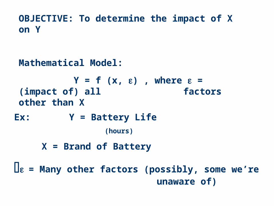
OBJECTIVE: To determine the impact of X on Y

Mathematical Model:

Y = f (x, ) , where = (impact of) all factors other than X

Ex: Y = Battery Life

(hours)

X = Brand of Battery

= Many other factors (possibly, some we’re unaware of)

1-Way ANOVA 4

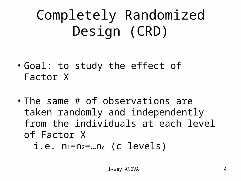
Completely Randomized Design (CRD)

4

• Goal: to study the effect of Factor X

• The same # of observations are taken randomly and independently from the individuals at each level of Factor X

i.e. n1=n2=…nc (c levels)

1-Way ANOVA 55

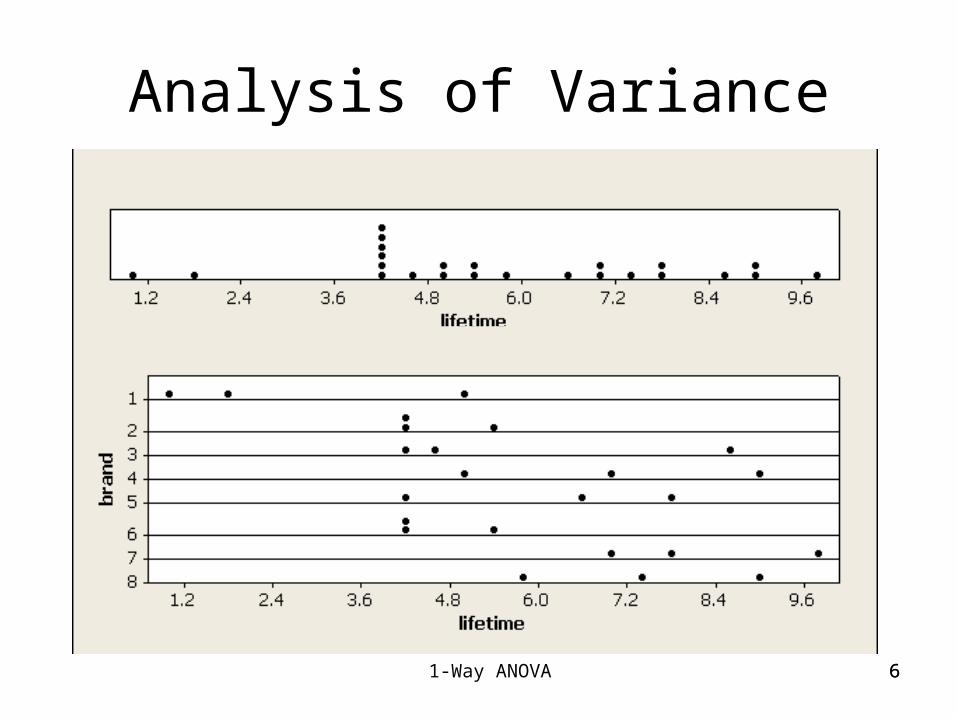
Example: Y = LIFETIME (HOURS)

BRAND3 replications

per level 1 2 3 4 5 6 7 8

1.8 4.2 8.6 7.0 4.2 4.2 7.8 9.0

5.0 5.4 4.6 5.0 7.8 4.2 7.0 7.4

1.0 4.2 4.2 9.0 6.6 5.4 9.8 5.8

2.6 4.6 5.8 7.0 6.2 4.6 8.2 7.4 5.8

1-Way ANOVA 6

Analysis of Variance

6

1-Way ANOVA 77

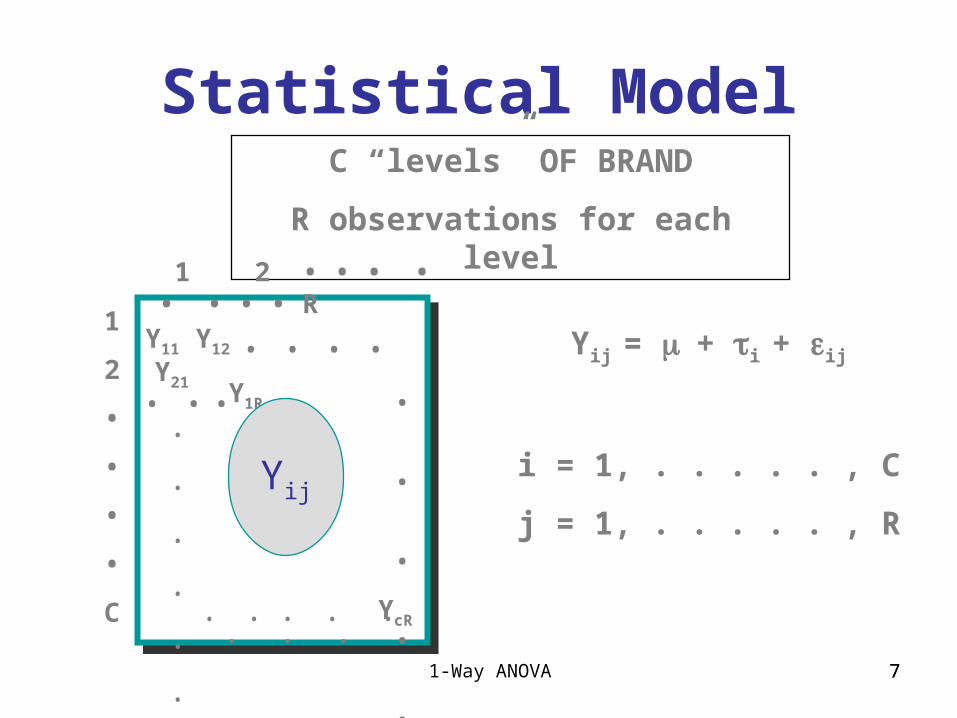
Statistical ModelC “levels” OF BRAND

R observations for each level

Y11 Y12 • • • • • • •Y1R

Yij

Y21

•

•

•

•

•

•

YcI

•

•

•

•

•

1

2

•

•

•

•

C

1 2 • • •  •  •  • • • R

Yij = + i + ij

i = 1, . . . . . , C

j = 1, . . . . . , R

YcR•   •  •   •    •   •    •    • 

1-Way ANOVA 88

Where

= OVERALL AVERAGE

i = index for FACTOR (Brand) LEVEL

j= index for “replication”

i = Differential effect associated with

ith level of X (Brand i) = i –

and ij = “noise” or “error” due to other factors associated with the (i,j)th data value.

i = AVERAGE associated with ith level of X (brand i)

= AVERAGE of i ’s.

1-Way ANOVA 99

Yij = + i + ij

By definition, i = 0C

i=1

The experiment produces

R x C Yij data values.

The analysis produces estimates of c. (We can then get estimates of

the ij by subtraction).

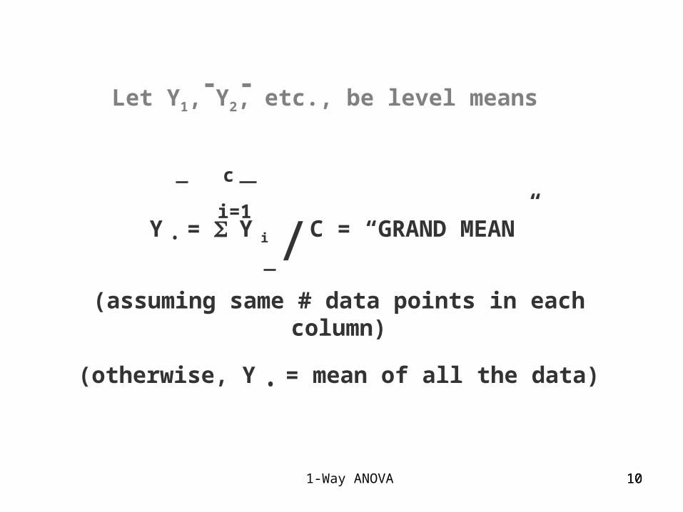
1-Way ANOVA 1010

Y • = Y i /C = “GRAND MEAN”

(assuming same # data points in each column)

(otherwise, Y • = mean of all the data)

i=1

c

Let Y1, Y2, etc., be level means

1-Way ANOVA 1111

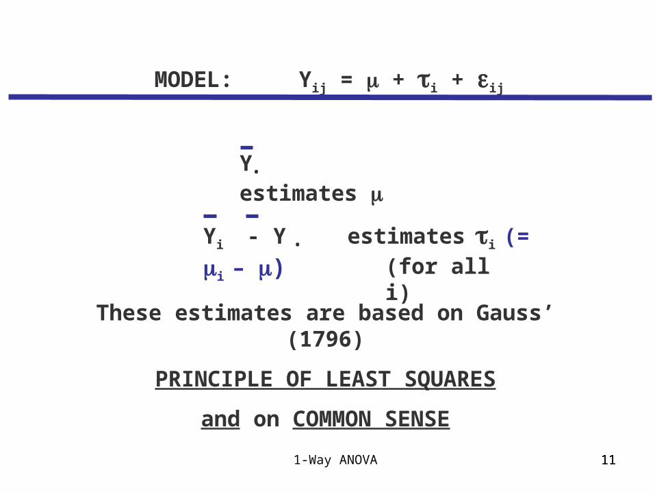
MODEL: Yij = + i + ij

Y• estimates

Yi - Y • estimatesi (= i – ) (for all i)

These estimates are based on Gauss’ (1796)

PRINCIPLE OF LEAST SQUARES

and on COMMON SENSE

1-Way ANOVA 1212

MODEL: Yij = + j + ij

If you insert the estimates into the MODEL,

(1) Yij = Y • + (Yj - Y • ) + ij.

it follows that our estimate of ij is

(2) ij = Yij – Yj, called residual

<

<

1-Way ANOVA 1313

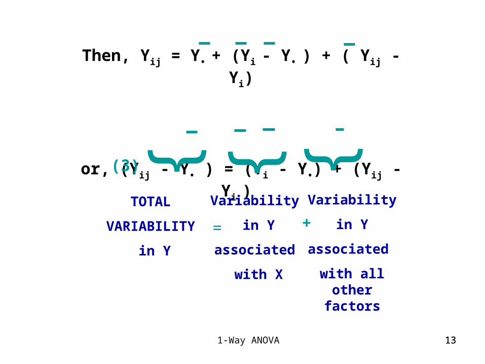
Then, Yij = Y• + (Yi - Y• ) + ( Yij - Yi)

or, (Yij - Y• ) = (Yi - Y•) + (Yij - Yi ) { { {(3)

TOTAL

VARIABILITY

in Y

=

Variability

in Y

associated

with X

Variability

in Y

associated

with all other factors

+

1-Way ANOVA 1414

If you square both sides of (3), and double sum both sides (over i and j), you get, [after some unpleasant algebra, but

lots of terms which “cancel”]

(Yij - Y• )2 = R • (Yi - Y•)

2 + (Yij - Yi)

2C R

i=1 j=1 { { {i=1

C C R

i=1 j=1

TSS

TOTAL SUM OF SQUARES

=

=

SSB

SUM OF SQUARES BETWEEN SAMPLES

+

+

SSW (SSE)

SUM OF SQUARES WITHIN SAMPLES( ( (

( ((

1-Way ANOVA 1515

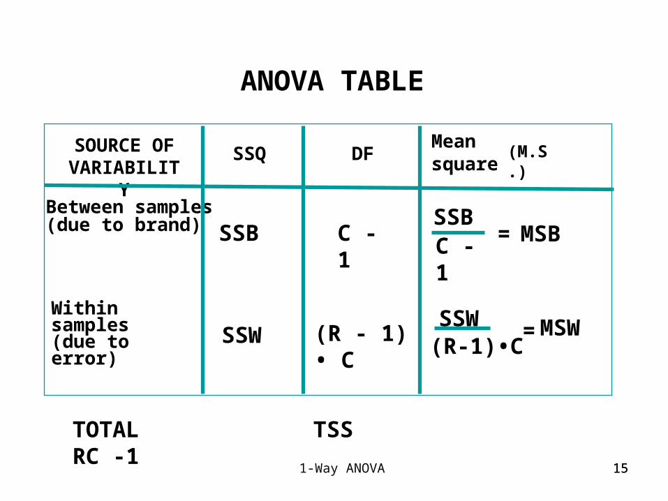
ANOVA TABLE

SOURCE OF VARIABILITY

SSQ DFMeansquare

(M.S.)

Between samples (due to brand)

Within samples (due to error)

SSB C - 1 MSBSSBC - 1

SSW (R - 1) • CSSW

(R-1)•C= MSW

=

TOTAL TSS RC -1

1-Way ANOVA 1616

Example: Y = LIFETIME (HOURS)

BRAND3 replications

per level 1 2 3 4 5 6 7 8

1.8 4.2 8.6 7.0 4.2 4.2 7.8 9.0

5.0 5.4 4.6 5.0 7.8 4.2 7.0 7.4

1.0 4.2 4.2 9.0 6.6 5.4 9.8 5.8

2.6 4.6 5.8 7.0 6.2 4.6 8.2 7.4 5.8

SSB = 3 ( [2.6 - 5.8]2 + [4.6 - 5.8]

2 + • • • + [7.4 - 5.8]2)

= 3 (23.04)

= 69.12

1-Way ANOVA 1717

(1.8 - 2.6)2 = .64 (4.2 - 4.6)2 =.16 (9.0 -7.4)2 = 2.56

(5.0 - 2.6)2 = 5.76 (5.4 - 4.6)2= .64 • • • • (7.4 - 7.4)2 = 0

(1.0 - 2.6)2 = 2.56 (4.2 - 4.6)2= .16 (5.8 - 7.4)2 = 2.56

8.96 .96 5.12

Total of (8.96 + .96 + • • • + 5.12),

SSW = 46.72

SSW =?

1-Way ANOVA 1818

ANOVA TABLE

Source of Variability

SSQ df M.S.

BRAND

ERROR

69.12

46.72

7

= 8 - 1

16

= 2 (8)

9.87

2.92

TOTAL 115.84 23

= (3 • 8) -1

1-Way ANOVA 1919

We can show:

E (MSB) = 2 +

“VCOL”{

MEASURE OF DIFFERENCES AMONG LEVEL

MEANS

RC-1

• (i - )2

{

i

((

E (MSW) = 2

(Assuming Yij follows N(j 2) and they are independent)

1-Way ANOVA 2020

E ( MSBC ) = 2 + VCOL

E ( MSW ) = 2

This suggests that

if MSBC

MSW > 1 ,

There’s some evidence of non-zero VCOL, or “level of X affects Y”

if MSBC

MSW< 1 ,

No evidence that VCOL > 0, or that “level of X affects Y”

1-Way ANOVA 2121

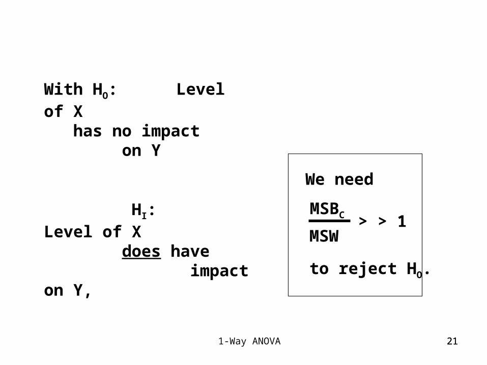
With HO: Level of X has no impact on Y

HI: Level of X does have impact on Y,

We need

MSBC

MSW> > 1

to reject HO.

1-Way ANOVA 2222

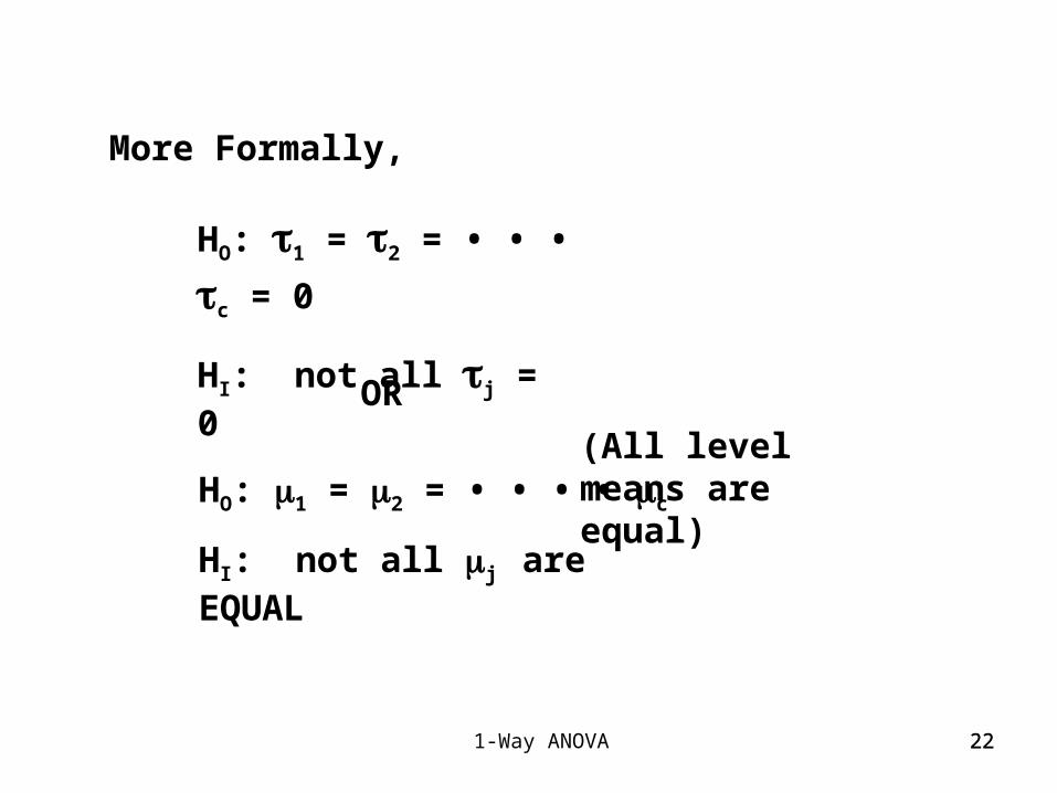
More Formally,

HO: 1 = 2 = • • • c = 0

HI: not all j = 0

OR

HO: 1 = 2 = • • • • c

HI: not all j are EQUAL

(All level means are equal)

1-Way ANOVA 2323

The distribution of

MSB

MSW= “Fcalc” , is

The F - distribution with (C-1, (R-1)C)degrees of freedom

Assuming

HO true.

C = Table Value

1-Way ANOVA 2424

In our problem:

ANOVA TABLE

Source of Variability

SSQ df M.S.

BRAND

ERROR

69.12

46.72

7

16

9.87

2.92 = 9.87 2.92

Fcalc

3.38

1-Way ANOVA 2525

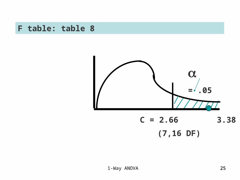
= .05

C = 2.66 3.38

F table: table 8

(7,16 DF)

1-Way ANOVA 2626

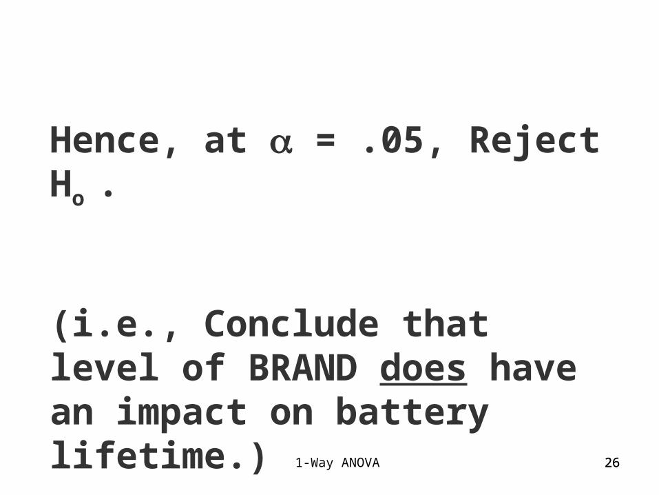
Hence, at = .05, Reject Ho .

(i.e., Conclude that level of BRAND does have an impact on battery lifetime.)

1-Way ANOVA 2727

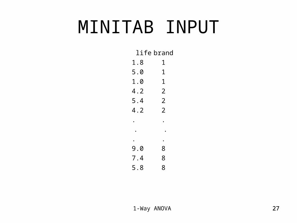
MINITAB INPUT life brand

1.8 1

5.0 1

1.0 1

4.2 2

5.4 2

4.2 2

. .

. .

. .

9.0 8

7.4 8

5.8 8

1-Way ANOVA 2828

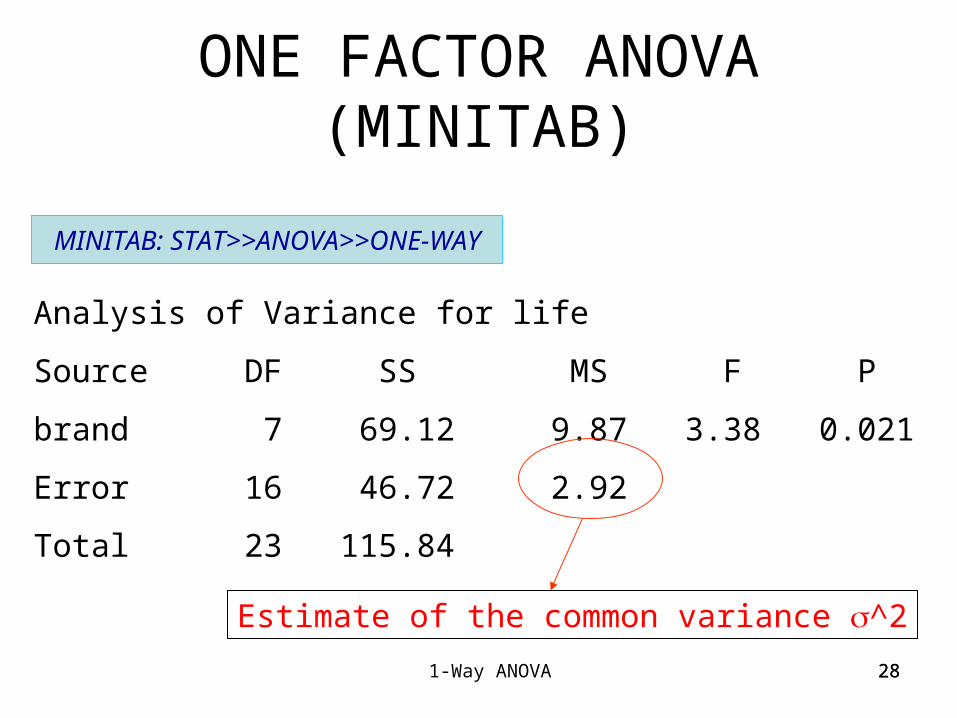
ONE FACTOR ANOVA (MINITAB)

Analysis of Variance for life

Source DF SS MS F P

brand 7 69.12 9.87 3.38 0.021

Error 16 46.72 2.92

Total 23 115.84

MINITAB: STAT>>ANOVA>>ONE-WAY

Estimate of the common variance ^2

1-Way ANOVA 2929

1 2 3 4 5 6 7 8

0

1

2

3

4

5

6

7

8

9

10

brand

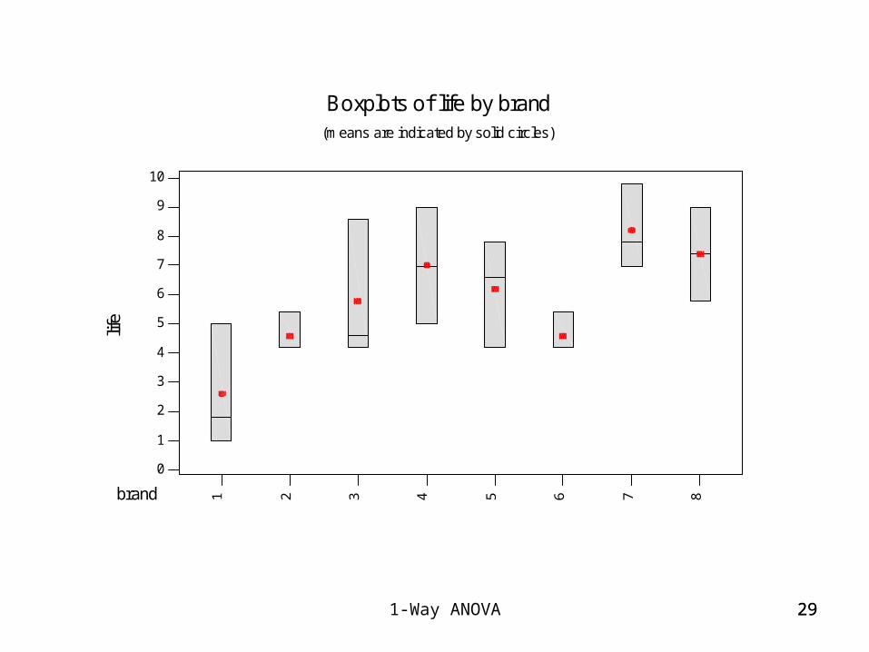
lifeBoxplots of life by brand

(means are indicated by solid circles)

1-Way ANOVA 3030

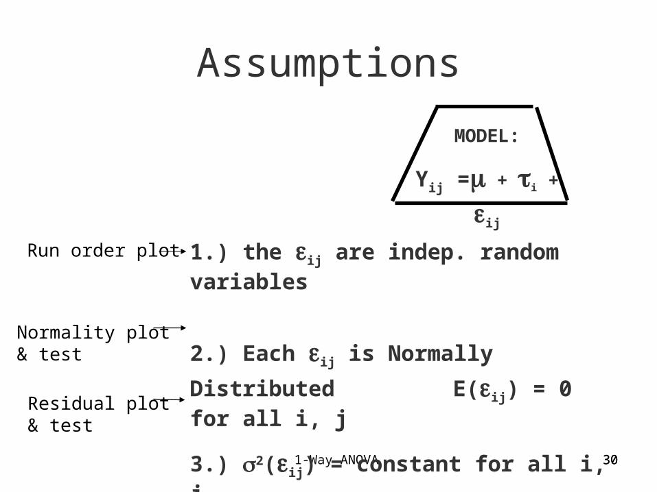
Assumptions

MODEL:

Yij = + i + ij

1.) the ij are indep. random variables

2.) Each ij is Normally Distributed

E(ij) = 0 for all i, j

3.) 2(ij) = constant for all i, j

Normality plot& test

Residual plot& test

Run order plot

1-Way ANOVA 3131

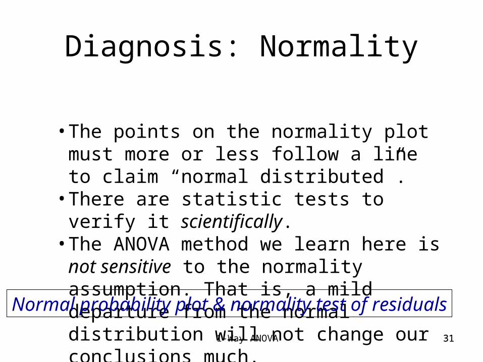
Diagnosis: Normality

• The points on the normality plot must more or less follow a line to claim “normal distributed”.

• There are statistic tests to verify it scientifically. • The ANOVA method we learn here is not

sensitive to the normality assumption. That is, a mild departure from the normal distribution will not change our conclusions much.

Normal probability plot & normality test of residuals

1-Way ANOVA 3232

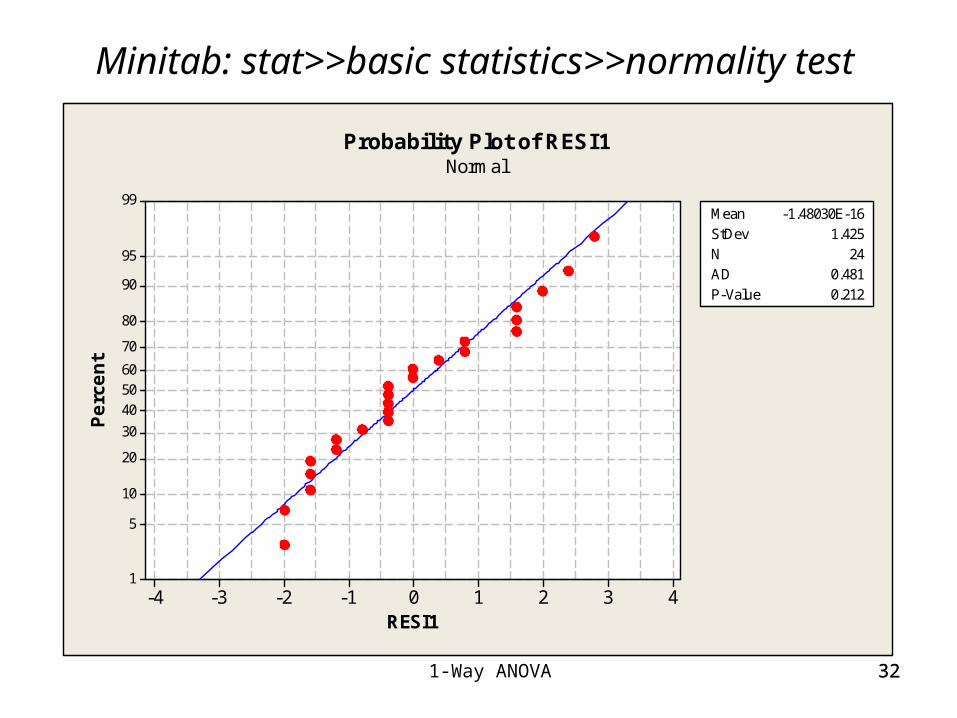
Minitab: stat>>basic statistics>>normality test

RESI1

Perc

ent

43210-1-2-3-4

99

95

90

80

70

605040

30

20

10

5

1

Mean -1.48030E-16StDev 1.425N 24AD 0.481P-Value 0.212

Probability Plot of RESI1Normal

1-Way ANOVA 3333

Diagnosis: Constant Variances

• The points on the residual plot must be more or less within a horizontal band to claim “constant variances”.

• There are statistic tests to verify it scientifically. • The ANOVA method we learn here is not sensitive

to the constant variances assumption. That is, slightly different variances within groups will not change our conclusions much.

Tests and Residual plot: fitted values vs. residuals

1-Way ANOVA 3434

Minitab: Stat >> Anova >> One-way

Fitted Value

Resi

dual

8765432

3

2

1

0

-1

-2

Residuals Versus the Fitted Values(response is life)

1-Way ANOVA 3535

Minitab: Stat>> Anova>> Test for Equal variancesbra

nd

95% Bonferroni Confidence Intervals for StDevs

8

7

6

5

4

3

2

1

403020100

Test Statistic 4.20P-Value 0.757

Test Statistic 0.31P-Value 0.938

Bartlett's Test

Levene's Test

Test for Equal Variances for life

1-Way ANOVA 3636

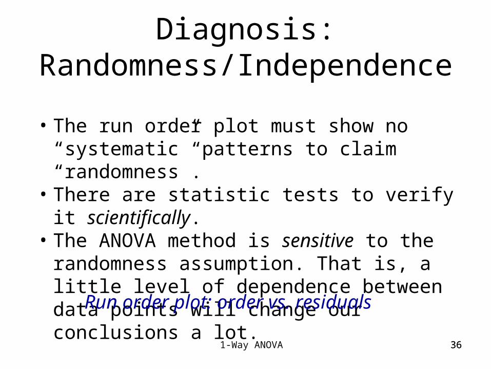
Diagnosis: Randomness/Independence

• The run order plot must show no “systematic” patterns to claim “randomness”.

• There are statistic tests to verify it scientifically. • The ANOVA method is sensitive to the randomness

assumption. That is, a little level of dependence between data points will change our conclusions a lot.

Run order plot: order vs. residuals

1-Way ANOVA 3737

Observation Order

Resi

dual

24222018161412108642

3

2

1

0

-1

-2

Residuals Versus the Order of the Data(response is life)

Minitab: Stat >> Anova >> One-way

1-Way ANOVA 3838

KRUSKAL - WALLIS TEST

(Non - Parametric Alternative)

HO: The probability distributions are identical for each level of the factor

HI: Not all the distributions are the same

1-Way ANOVA 3939

Brand

A B C

32 32 28

30 32 21

30 26 15

29 26 15

26 22 14

23 20 14

20 19 14

19 16 11

18 14 9

12 14 8

BATTERY LIFETIME (hours)

(each column rank ordered, for simplicity)

Mean: 23.9 22.1 14.9 (here, irrelevant!!)

1-Way ANOVA 4040

HO: no difference in distribution among the three brands with

respect to battery lifetime

HI: At least one of the 3 brands differs in distribution from the others with respect to lifetime

1-Way ANOVA 4141

Brand

A B C

32 (29) 32 (29) 28 (24)

30 (26.5) 32 (29) 21 (18)

30 (26.5) 26 (22) 15 (10.5)

29 (25) 26 (22) 15 (10.5)

26 (22) 22 (19) 14 (7)

23 (20) 20 (16.5) 14 (7)

20 (16.5) 19 (14.5) 14 (7)

19 (14.5) 16 (12) 11 (3)

18 (13) 14 (7) 9 (2)

12 (4) 14 (7) 8 (1)T1 = 197 T2 = 178 T3 = 90

n1 = 10 n2 = 10 n3 = 10

Ranks in ( )

1-Way ANOVA 4242

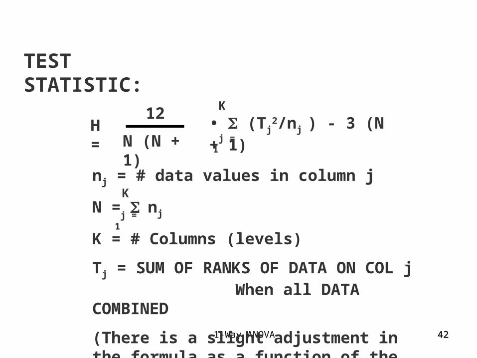
TEST STATISTIC:

H =12

N (N + 1)• (Tj

2/nj ) - 3 (N + 1)

nj = # data values in column j

N = nj

K = # Columns (levels)

Tj = SUM OF RANKS OF DATA ON COL j When all DATA COMBINED

(There is a slight adjustment in the formula as a function of the number of ties in rank.)

K

j = 1

K

j = 1

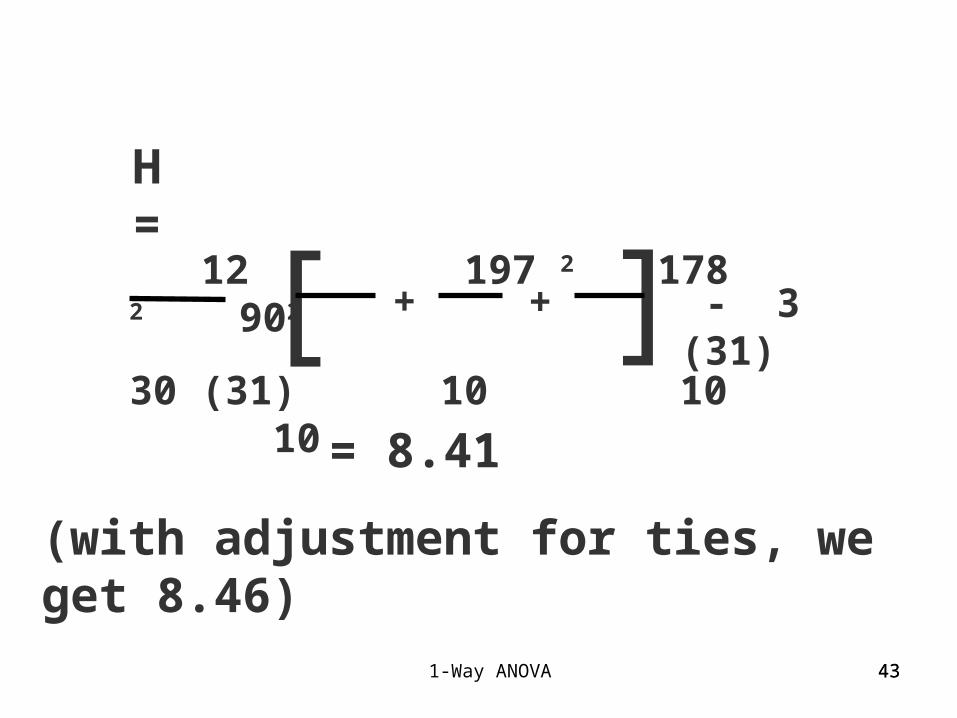
1-Way ANOVA 4343

H =

[ 12 197 2 178 2 902

30 (31) 10 10 10+ +

[ - 3 (31)

= 8.41

(with adjustment for ties, we get 8.46)

1-Way ANOVA 4444

We can show that, under HO , H is well

approximated by a 2 distribution with df = K - 1.

What do we do with H?

Here, df = 2, and at = .05, the critical value = 5.99

2

df

dfFdf,=

5.99 8.41 = H

= .05

Reject HO; conclude that mean lifetime NOT the same for all 3 BRANDS

8

1-Way ANOVA 4545

• Kruskal-Wallis Test: life versus brand

• Kruskal-Wallis Test on life

• brand N Median AveRank Z• 1 3 1.800 4.5 -2.09• 2 3 4.200 7.8 -1.22• 3 3 4.600 11.8 -0.17• 4 3 7.000 16.5 1.05• 5 3 6.600 13.3 0.22• 6 3 4.200 7.8 -1.22• 7 3 7.800 20.0 1.96• 8 3 7.400 18.2 1.48• Overall 24 12.5

• H = 12.78 DF = 7 P = 0.078• H = 13.01 DF = 7 P = 0.072 (adjusted for ties)

Minitab: Stat >> Nonparametrics >> Kruskal-Wallis