1

UAV Routing and Coordination inStochastic, Dynamic Environments

John J. Enright Emilio FrazzoliMarco Pavone Ketan Savla

Abstract

Recent years have witnessed great advancements in the science and technology for unmanned aerial vehicles(UAVs), e.g., in terms of autonomy, sensing, and networking capabilities. This chapter surveys algorithms on taskassignment and scheduling for one or multiple UAVs in a dynamic environment, in which targets arrive at randomlocations at random times, and remain active until one of the UAVs flies to the target’s location and performs anon-site task. The objective is to minimize some measure of the targets’ activity, e.g., the average amount of timeduring which a target remains active. The chapter focuses on a technical approach that relies upon methods fromqueueing theory, combinatorial optimization, and stochastic geometry. The main advantage of this approach is itsability to provide analytical estimates of the performance of the UAV system on a given problem, thus providinginsight into how performance is affected by design and environmental parameters, such as the number of UAVsand the target distribution. In addition, the approach provides provable guarantees on the system’s performancewith respect to an ideal optimum. To illustrate this approach, a variety of scenarios are considered, ranging fromthe simplest case where one UAV moves along continuous paths and has unlimited sensing capabilities, to the casewhere the motion of the UAV is subject to curvature constraints, and finally to the case where the UAV has a finitesensor footprint. Finally, the problem of cooperative routing algorithms for multiple UAVs is considered, withinthe same queueing-theoretical framework, and with a focus on control decentralization.

I. INTRODUCTION

This chapter discusses current solution approaches for the design of cooperative control and taskallocation strategies for networks of unmanned aerial vehicles (UAVs). The focus is on uncertain anddynamically changing environments, in which new task requests are generated in real time, and on routingalgorithms with performance guarantees, as opposed to heuristic algorithms.

As a motivating example, consider the following scenario: a team of Unmanned Aerial Vehicles (UAVs)is responsible to investigate possible threats over a region of interest. As possible threats are detected,by intelligence, high-altitude or orbiting platforms, or by ground sensor networks, one of the UAVs mustvisit its location and investigate the cause of the alarm, in order to enable an appropriate response ifnecessary. Performing this task may require the UAV not only to fly to the possible threat’s location, butalso to spend additional time on site. The objective is, in general, to minimize the average time betweenthe appearance of a possible threat and the time one of the UAVs completes the close-range inspectiontask. In a variation of this problem, which will be referred to as persistent patrolling, the UAVs mustdetect possible threats using limited-range on-board sensors. Other variations may include priority levelsor time windows during which the inspection task must be completed.

In order to perform the required mission, the UAVs (or, more in general, mission control) need torepeatedly solve three coupled decision-making problems:

1) Task allocation among the UAVs: Which UAV shall pursue each task? What policy is used toassign tasks to UAVs?,

Senior Research Scientist, Kiva Systems jenright@kivasystems.com.Associate Professor, Laboratory for Information and Decision Systems, Aeronautics and Astronautics Department, Massachusetts Institute

of Technology frazzoli@mit.edu.Assistant Professor, Aeronautics and Astronautics Department, Stanford University pavone@stanford.edu

Assistant Professor, Sonny Astani Department of Civil and Environmental Engineering, University of Southern Californiaksavla@usc.edu.

2

2) Service scheduling for each UAV: Given the list of tasks to be pursued, what is the most efficientordering of these tasks?

3) Loitering paths: What should UAVs without pending assignments do?In general, the combined problem, which one can refer to as Dynamic Vehicle Routing, falls within

the class of heterogeneous, stochastic (possibly distributed) decision-making problems with uncertaininformation, with additional complexity stemming from the differential and algebraic constraints on theUAV motion and the local sensing of the environment. This problem is generally intractable, and solutionapproaches have been devised that look either at heuristics algorithms or at approximation algorithmswith some guarantee on their performance.

The chapter is structured as follows. Section II presents an overview of current solution approaches forUAV routing in uncertain and dynamic environments. First, the differences and commonalities betweenstatic and dynamic UAV routing problems are discussed. Then, some of the main classes of algorithms usedin the relevant literature are introduced, namely, heuristic algorithms (without performance guarantees),as well as online algorithms and spatial queueing theory (which provide guaranteed approximations tooptimal performance). Section III considers in some detail the application of spatial queueing theory tosome prototypical scenarios, involving a single UAV. The main motivation is to show how to model aspecific UAV routing problem within this framework and how to solve it. Section IV considers the samescenarios, extending the theory to the case of multiple UAVs. Finally, Section V summarizes the chapter.

II. APPROACHES FOR UAV ROUTING IN DYNAMIC ENVIRONMENTS

The objective of this section is to first discuss the differences between static and dynamic environments,and then to present a broad overview of current solution approaches. Broadly speaking, there are threemain approaches available in the literature to tackle such Dynamic Vehicle Routing problems. The firstapproach relies on heuristic algorithms. In the second approach, called “online algorithms,” routing policiesare designed to minimize the worst-case ratio between their performance and the performance of an optimaloffline algorithm which has a priori knowledge of the entire input sequence. In the third approach, therouting problem is embedded within the framework of queueing theory, and routing policies are designedto minimize typical queueing-theoretical cost functions such as the expected time the tasks remain in thequeue. Since the generation of tasks and motion of the vehicles is within an Euclidean space, one canrefer to this third approach as spatial queueing theory.

A. Static and Dynamic Vehicle RoutingIn the recent past, considerable efforts have been devoted to the problem of how to cooperatively

assign and schedule tasks that are defined over an extended geographical area (Alighanbari and How,2008; Arslan et al., 2007; Beard et al., 2002; Moore and Passino, 2007; Smith and Bullo, 2009). In thesepapers, the main focus is in developing distributed algorithms that operate with knowledge about the tasklocations and with limited communication between robots. However, the underlying mathematical modelis static, in that no new tasks arrive over time, and fits within the framework of the static vehicle routingproblem, whereby: (i) a team of m vehicles is required to service a set of n tasks in a 2-dimensionalspace; (ii) each task requires a certain amount of on-site service; (iii) the goal is to compute a set of routesthat minimizes the cost of servicing the tasks; see Toth and Vigo (2001) for a thorough introduction tothis problem. In general, most of the available literature on routing for robotic networks focuses on staticenvironments and does not properly account for scenarios in which dynamic, stochastic and adversarialevents take place.

The problem of planning routes through service tasks that arrive during a mission execution is knownas the “dynamic vehicle routing problem” (abbreviated as the DVR problem in the operations researchliterature). There are two key differences between static and dynamic vehicle routing problems. First,planning algorithms should actually provide policies (in contrast to pre-planned routes) that prescribe howthe routes should evolve as a function of those inputs that evolve in real time. Second, dynamic tasks

3

Fig. 1. An illustration of dynamic routing problems for a robotic system. From left to right: (i) tasks are generated, (ii) vehicles are assignedto tasks and select routes, (iii) new tasks appear, requiring an update to assignments and routes.

(i.e., tasks that arrive and vary over time) add queueing phenomena to the combinatorial nature of vehiclerouting. In such a dynamic setting, it is natural to focus on steady-state performance instead of optimizingthe performance for a single task. Additionally, system stability in terms of the number of waiting tasksis an issue to be addressed.

B. Heuristic AlgorithmsA naıve, yet reasonable approach to devise an heuristic algorithm (i.e., an algorithm without performance

guarantees) would be to adapt classic queueing policies to spatial queueing systems. However, perhapssurprisingly, this adaptation is not at all straightforward. For example, policies based on a First-Come First-Served discipline, whereby tasks are fulfilled in the order in which they arrive, are unable to stabilizethe system for all stabilizable task arrival rates, in the sense that under such policies the average numberof tasks grows over time without bound, even though there exist other policies that would maintain thenumber of tasks uniformly bounded (Bertsimas and van Ryzin, 1991).

The most widely applied approach is to combine static routing methods (e.g., VRP-like methods orheuristic methods such as nearest neighbor or genetic algorithms) and sequential re-optimization, wherethe re-optimization horizon is chosen heuristically. (A similar approach, incidentally, is at the core also ofthe approximation algorithms presented in the following sections.) However, the joint selection of a staticrouting method and of the re-optimization horizon in presence of UAV and task constraints (e.g., differentialmotion constraints, or task priorities) makes the application of this approach far from trivial. First, one canshow that an erroneous selection of the re-optimization horizon can lead to pathological scenarios whereno task ever receives service (Pavone, 2010). Second, direct application of VRP-like methods might leadto infeasible paths for vehicles with differential motion constraints. Additionally, performance criteria indynamic settings commonly differ from those of the corresponding static problems. For example, in adynamic setting, the time needed to complete a task may be a more important factor than the total vehicletravel cost.

C. Online AlgorithmsAn online algorithm is one that operates based on input information available up to the current time.

Thus, these algorithms are designed to operate in scenarios where the entire input is not known at theoutset, and new pieces of the input should be incorporated as they become available. The distinctivefeature of the online algorithm approach is the method used to evaluate an algorithm’s performance,which is called competitive analysis (Sleator and Tarjan, 1985). In competitive analysis, the performanceof an online algorithm is compared to the performance of a corresponding offline algorithm (i.e., analgorithm that has a priori knowledge of the entire input) in the worst-case scenario. Specifically, anonline algorithm is c-competitive if its cost on any problem instance is at most c times the cost of anoptimal offline algorithm:

Costonline(I) c Costoptimal offline(I), 8 problem instances I.

4

In the recent past, several dynamic vehicle routing problems have been successfully studied in thisframework, under the name of the online traveling repairman problem (Irani et al., 2004; Jaillet andWagner, 2006; Krumke et al., 2003), and many interesting insights have been obtained. However, the onlinealgorithm approach has some disadvantages. First, competitive analysis is a worst-case analysis, hence, theresults are often overly pessimistic for normal problem instances. Moreover, in many applications thereis some probabilistic problem structure (e.g., distribution of the inter-arrival times, spatial distributionof future tasks, distribution of on-site service times etc.), that can be advantageously exploited by thevehicles. In online algorithms, this additional information is not taken into account. Second, competitiveanalysis is used to bound the performance relative to the optimal offline algorithm, and thus it does notgive an absolute measure of performance. In other words, an optimal online algorithm is an algorithm withminimum “cost of causality” in the worst-case scenario, but not necessarily with the minimum worst-casecost. Finally, many important real-world constraints for DVR, such as time windows, priorities, differentialconstraints on vehicle’s motion and the requirement of teams to fulfill a task “have so far proved to betoo complex to be considered in the online framework” (Golden et al., 2008, page 206). Some of thesedrawbacks have been recently addressed by Van Hentenryck et al. (2009) where a combined stochastic andonline approach is proposed for a general class of combinatorial optimization problems and is analyzedunder some technical assumptions.

D. Spatial Queueing TheorySpatial queueing theory embeds the dynamic vehicle routing problem within the framework of queueing

theory and overcomes some of the limitations of the online algorithm approach; in particular, it allowsto take into account several real-world constraints, such as time constraints and priorities. The namespatial queueing theory stems from the fact that the generation of the tasks and the motion of the servers(i.e., UAVs) happens in a metric space. This chapter concentrates on an algorithmic approach to spatialqueueing theory whose objective is to synthesize an efficient control policy, whereas in standard queueingtheory the objective is usually to analyze the performance of a specific policy. Within this context, anefficient policy is one whose expected performance is either optimal or within a constant factor of theoptimum. Specifically, the expected performance of a policy is the expected value of the performanceover all possible inputs (i.e., task arrival sequences). A policy performs within a constant factor of theoptimum if the ratio between the policy’s expected performance and the optimal expected performance isupper bounded by .

In order to make the model tractable, tasks are usually considered “statistically independent” and theirarrival process is assumed stationary (with possibly unknown parameters). These assumptions, however,can be unrealistic in some scenarios, in which case the online algorithms approach may represent a betteralternative. Pioneering work in this context is that of Bertsimas and van Ryzin (1991, 1993a,b), whointroduced queueing methods to solve the simplest DVR problem (a vehicle moves along straight linesand visits tasks whose time of arrival, location and on-site service are stochastic; information about tasklocation is communicated to the vehicle upon task arrival); see also the earlier related work (Psaraftis,1980). Recently, by integrating ideas from dynamics, combinatorial optimization, teaming, and distributedalgorithms, this approach has been applied to scenarios with complex models for the tasks such as timeconstraints, service priorities and translating tasks, problems concerning robotic implementation such asadaptive and decentralized algorithms, complex vehicle dynamics, limited sensing range, and team forming,and even integration of humans in the design space, see Bullo et al. (2011) and references therein.

An interesting feature of this approach is that the performance analysis of these algorithms usuallyyields scaling laws for quality of performance in terms of mission parameters. These scaling laws canserve as useful guidelines for operators to select mission parameters when feasible (e.g., number of UAVs,sensing range, etc.) to provide a desired quality of service.

5

III. SPATIAL QUEUEING THEORY: THE SINGLE-SERVER CASE

This section presents the basic ideas and tools for an algorithmic approach to spatial queuing theory(more details can be found in, e.g., Bullo et al. (2011)). This approach consists of three main steps, namelydevelopment of a spatial queueing model, establishment of fundamental limitations of performance, anddesign of algorithms with performance guarantees. More specifically, the formulation of a model entailsdetailing four main aspects:

1) A model for the dynamic component of the environment: this is usually achieved by assuming thatnew events are generated (either adversarially or stochastically) by an exogenous process.

2) A model for targets/tasks: tasks are usually modeled as points in a physical environment distributedaccording to some (possibly unknown) distribution, might require a certain level of on-site servicetime, and can be subject to a variety of constraints, e.g., time windows, priorities, etc.

3) A model for the UAVs and their motion: besides their number, one needs to specify whetherthe UAVs are subject to algebraic (e.g., obstacles) or differential (e.g., minimum turning radius)constraints, sensing constraints, and fuel constraints. Also, UAVs might be able to communicatedirectly only with other UAVs (or static nodes) that lie within a certain radius, or might not haveany communication capability (e.g., when cheap micro-UAVs are used, or stealthiness is required).Finally, the control could be centralized (i.e., coordinated by a central station) or decentralized.

4) Performance criterion: examples include the minimization of the waiting time before service, lossprobabilities, expectation-variance analysis, etc.

Once the model is formulated, one seeks to characterize fundamental limitations of performance (in theform of lower bounds for the best achievable cost); the purpose of this step is essentially twofold: itallows to quantify the degree of optimality of a routing algorithm and provides structural insights into theproblem. As for the last step, the design of a routing algorithm usually relies on a careful combination ofstatic routing methods with sequential re-optimization. Desirable properties for the static methods are: (i)the static problem can be solved (at least approximately) in polynomial time, and (ii) the static methodis amenable to a statistical characterization (this is essential for the computation of performance bounds).Formal performance guarantees on a routing algorithm are then obtained by quantifying the ratio betweenan upper bound on the cost delivered by that algorithm and a lower bound for the best achievable cost.Such a ratio, being an estimate of the degree of optimality of the algorithm, should be close to one andpossibly independent of systems’s parameters (i.e., a constant factor guarantee, as defined in Section II).

In the remainder of this section, three problems will be considered, all involving only one UAV (theserver in the queueing model: in the remainder of this chapter the terms “server” and “UAV,” as well as“task” and “target,” will be used interchangeably). In the first problem the UAV moves along continuouspaths and visits targets whose time of arrival, location and on-site service are stochastic; information abouttarget location is communicated to the UAV upon target arrival. In the second problem, the motion of theUAV is subject to differential constraints, but still the UAV has full knowledge of newly arrived targets.Finally, in the third problem, the information available to the UAV is limited, i.e., the UAV is not awareof a target’s existence or location upon its arrival time, but must first detect it using on-board sensors.

The purpose of these examples is twofold: on the one hand, to provide some concrete examples abouthow to apply spatial queuing theory to devise UAV routing algorithms in dynamic settings, on the otherhand to provide guidelines for UAV routing in a variety of scenarios of interest. The case of multi-UAVcoordination will be addressed in the next section.

A. UAV routing with no motion constraints and unlimited sensingConsider a basic scenario where one UAV moves along continuous paths (with no differential constraints,

e.g., on the curvature) and visits spatially-localized targets whose time of arrival, location and on-siteservice are stochastic; information about target location is communicated to each UAV upon target arrival.This problem has been studied in the literature as the Dynamic Traveling Repairman Problem (DTRP) inBertsimas and van Ryzin (1991), and can be summarized as follows:

6

The single-server DTRP problem: In a geographical region Q of area A, a dynamic process generatesspatially localized tasks. The process generating tasks is modeled as a spatio-temporal Poisson process,i.e., (i) the time between each pair of consecutive events has an exponential distribution with intensity� > 0 and (ii) upon arrival, the locations of tasks are independently and uniformly distributed in Q.The location of the new tasks is assumed to be immediately available to the UAV. The UAV providesservice in Q, flying at constant speed v; the UAV is assumed to have unlimited fuel and task-servicingcapabilities. Each task requires an independent and identically distributed amount of on-site service withfinite mean duration s > 0. A task is completed when the UAV moves to its location and performs itson-site service. The objective is to design a routing policy that maximizes the Quality of Service deliveredby the UAV in terms of the average steady-state time delay T between the generation of a task and thetime it is completed (in general, in a dynamic setting, the focus is on the quality of service as perceivedby the “end user,” rather than, for example, fuel economies achieved by the UAV). Other quantities ofinterests are the average number N of tasks waiting to be completed and the waiting time W of a taskbefore its location is reached by a UAV. These quantities, however, are related according to T = W + s(by definition) and by Little’s law, stating that N = �W , for stable queues (Little, 1961).

One comment is in order: the queueing models used to model UAV routing problems are inherentlydifferent from traditional, non-spatial queuing models. In particular, one might be tempted to considerthe queuing model for the single-server DTRP as a standard M/G/1 queue (where M stands for Poissonarrival process, G indicates that the service times are identically and independently distributed accordingto a general distribution, and 1 is the number of servers). The main reason is that in UAV routing the“service time” has both a travel and an on-site component. Although the on-site service requirements are“statistically” independent (by assumption), the travel times generally are not.

Stability: Before proceeding further, it is necessary to ensure the stability of the system. The system isconsidered stable if the expected number of waiting tasks is uniformly bounded at all times, or equivalently,that tasks are removed from the system at least at the same rate at which they are generated. In the caseat hand, the time to complete a task is the sum of the time to reach its location (which depends onthe routing policy) plus the time spent at that location in on-site service (which is independent of therouting policy). Since, by definition, the service time is no shorter than the on-site service time s, then aweaker necessary condition for stability is % := �s < 1; the quantity % measures the fraction of time theUAV is performing on-site service. Remarkably, it turns out that this is also a sufficient condition for thesingle-server DTRP; note that this stability condition is independent of the size and shape of Q, and ofthe speed of the vehicle.

Lower bounds: To derive lower bounds, the main difficulty usually consists in bounding (possibly ina statistical sense) the amount of time spent to reach a target location. The derivation of these boundsbecomes simpler in asymptotic regimes, i.e., looking at cases when % ! 0

+ and % ! 1

�, which are oftencalled “light load” and “heavy load” conditions, respectively.

For example, consider first the case in which % ! 0

+ (light load regime). The median of Q is definedas the point that minimizes the expected distance to a random point sampled uniformly from Q; thisdistance can be written as H⇤

1

pA, where H⇤

1

is a constant that only depends on the shape of Q (see alsoAppendix A). Assuming that the UAV would have enough time to return to the median location beforethe appearance of each new task (in other words, assuming light load conditions), the expected systemtime can be lower bounded as

T � H⇤1

pA

v+ s (as % ! 0

+

).

Consider now the case in which % ! 1

� (heavy load). Let D be the average travel distance per taskfor some routing policy. By using arguments from geometrical probability (independent of algorithms),one can show that D � �

2

pA/

p2N as % ! 1

�, where �2

is a constant that will be specified later. Asdiscussed, for stability one needs s +D/v < 1/�. Combining the stability condition with the bound onthe average travel distance per task, one obtains

7

s+�2

pA

vp2N

1

�.

Since, by Little’s law, N = �W and T = W + s, one finally obtains (recall that % = �s):

T � �2

2

2

A

v2�

(1 � %)2+ s, (as % ! 1

�).

This lower bound allows to draw the following conclusions for the single-server DTRP: (i) the condition% < 1 is also sufficient for stability, and (ii) the Quality of Service, which is proportional to 1/(1 � %)2,degrades much faster as the target load increases than in a non-spatial queueing systems (where the growthrate is proportional to 1/(1 � %)).

Routing for the single-server DTRP: Consider the following routing policy for the single-server DTRP,based on a partition of Q into p � 1 sub-regions {Q

1

, Q2

, . . . , Qp} of equal area A/p. Such a partitioncan be obtained, e.g., as sectors centered at the median of Q. Define a cyclic ordering for the sub-region,such that, e.g., if the vehicle is in region Qi the “next” region is Qj , where j follows i in the cyclicordering (in other words, j = (i+ 1)modp).

1) If there are no outstanding targets, move to the median of the region Q.2) Otherwise, visit the “next” sub-region; subregions with no tasks are skipped. Compute a

minimum-length path from the UAV’s current position through all the outstanding tasks inthat subregion. Complete all tasks on this path, ignoring new tasks generated in the meantime.

3) Repeat.

In the above policy, two static optimization methods are applied, depending on whether or not thereare outstanding tasks. Computing the median of Q is a standard problem in geometric optimization (seeAppendix A). The problem of computing the shortest path through a number of points is related to thewell-known Traveling Salesman Problem (TSP). While the TSP is a prototypically hard combinatorialproblem, it is well known that the Euclidean version of the problem is very easy to approximate; seeAppendix B for more details. Furthermore, the length ETSP(n) of a Euclidean TSP through n pointsindependently and uniformly sampled in Q is known to satisfy the following property:

lim

n!1ETSP(n)/

pn = �

2

·pA, almost surely,

where �2

⇡ 0.712 is a constant; this is the same constant that appears in the lower bound. The convergenceto this limit is very fast: Larson and Odoni (1981) report that for “fairly compact and fairly convex” regions,the estimate ETSP(n) ⇡ �

2

pnA is within a few percent from the true value for as few as 15 points.

It can be shown (see, e.g., Bertsimas and van Ryzin (1993a)) that, using the above routing policy, theaverage system time T satisfies

T =

H⇤1

pA

v+ s, (as % ! 0

+

),

T �(p)A

v2�

(1 � %)2+ s, (as % ! 1

�),

where �(1) = �2

2

, and �(p) ! �2

2

/2 for large p. These results critically exploit the statistical characteri-zation of the length of an optimal TSP tour. Hence, the proposed policy achieves a quality of service thatis arbitrarily close to the optimal one, in the asymptotic regimes of light or heavy load.

While the simple policy stated above is provably optimal in light and heavy load, in the sense that nopolicy can provide a strictly lower system time, several variations have been proposed that improve the

8

performance in other scenarios or operating conditions, at the expense of some additional complexity inimplementation and analysis. The interested reader can find more information in Bullo et al. (2011) andreferences therein.

B. UAV routing with motion constraints and unlimited sensingIn this section, the complexity of the single-server DTRP problem is increased, by imposing differential

constraints on the trajectories that the UAV can follow.The single-server Dubins DTRP problem: In this version of the problem, the task generation process

and performance metrics are assumed to be the same as in the standard DTRP problem. On the other hand,the UAV is modeled as a non-holonomic vehicle, constrained to move on the plane at constant speed v,along paths of bounded curvature. In particular, the instantaneous radius of curvature is constrained to beno less than ⇢. This model is often referred to as the Dubins vehicle, in recognition of Dubins’ work incomputing minimum-length paths for such model (Dubins, 1957), and is typically considered appropriateto model the kinematics of UAVs (Beard et al., 2002; Chandler et al., 2000). The UAVs are assumed tobe identical, and have unlimited range. In the course of this chapter, the term Dubins frame shall be usedto refer to a coordinate frame with the origin attached to the Dubins vehicle and its first axis aligned withthe vehicle’s velocity vector. For simplicity, the region Q will be assumed to be a rectangle of height Hand width W , with H < W , and WH = A. The on-site service time will be assumed to be identicallyzero, e.g., as in fly-by requests. This version of the DTRP will be henceforth called the Dubins DTRP.

Lower bounds: The lower bounds from the basic case still hold. Note that in this case, since s = 0,the load is entirely determined by �: in the light-load case � ! 0

+, and in the heavy-load case � ! +1.So, for example, the light-load lower bound is

T � H⇤1

/v, (as � ! 0

+

).

For the heavy-load case, it is possible to derive a lower bound specific to the Dubins DTRP. Let D⇢(n)be the expected distance along a Dubins path, between a UAV situated in the interior of Q and the closestamong n points independently and uniformly sampled from Q. Reachability arguments show that, forlarge n,

D⇢(n) � �D

✓

⇢A

n

◆

1/3

,

where �D

=

3

4

3p3. In the case s = 0, stability requires D⇢(N)/v 1/�, and Little’s condition states that

N = �T . Hence, for large �,1

�� D⇢(N)

v� �

D

✓

⇢A

�T

◆

1/31

v,

and finallyT � �3

D

⇢A

v3�2, (as � ! +1).

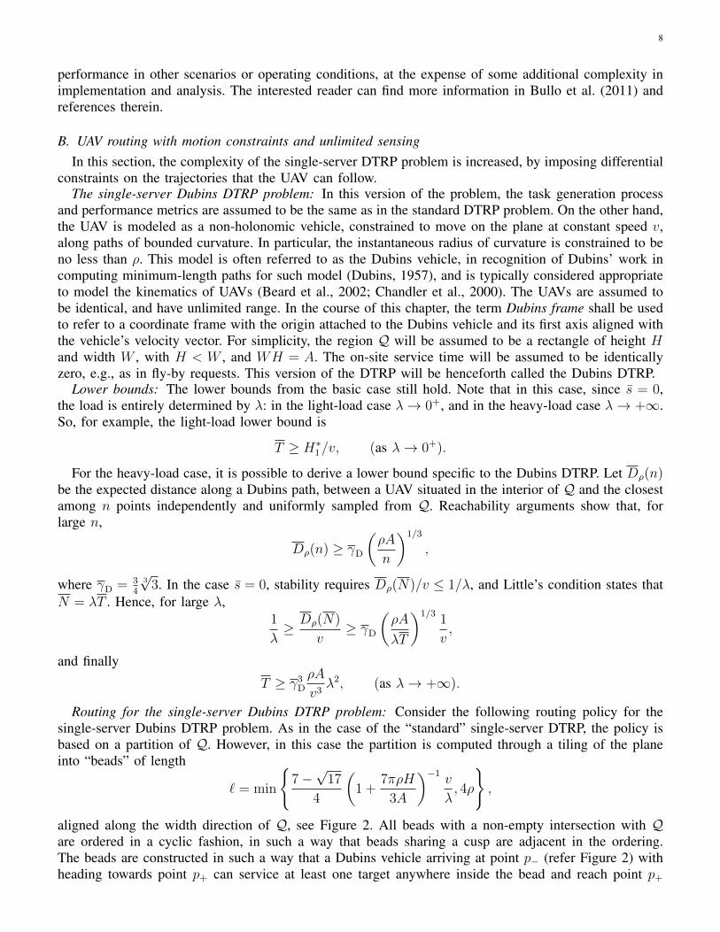
Routing for the single-server Dubins DTRP problem: Consider the following routing policy for thesingle-server Dubins DTRP problem. As in the case of the “standard” single-server DTRP, the policy isbased on a partition of Q. However, in this case the partition is computed through a tiling of the planeinto “beads” of length

` = min

(

7 �p17

4

✓

1 +

7⇡⇢H

3A

◆�1

v

�, 4⇢

)

,

aligned along the width direction of Q, see Figure 2. All beads with a non-empty intersection with Qare ordered in a cyclic fashion, in such a way that beads sharing a cusp are adjacent in the ordering.The beads are constructed in such a way that a Dubins vehicle arriving at point p� (refer Figure 2) withheading towards point p

+

can service at least one target anywhere inside the bead and reach point p+

9

with the same heading as it had when it arrived at point p�. This feature allows the Dubins vehicle toservice at least one target per bead in a cyclic fashion.

⇢

p� p+B�(�)

�

(a) (b)

Fig. 2. (a) Construction of the “bead”. The figure shows how the upper half of the boundary is constructed, the bottom half is symmetric.(b) Bead tiling of the plane, with the beads aligned with the width of Q.

1) If there are no outstanding targets, loiter on a circular trajectory of radius ⇢ about the medianof the region Q. The direction of loitering is irrelevant, and can be chosen in such a way thatthe loitering circle is returned to in minimum time after servicing the target.

2) Otherwise, visit beads in order, servicing at least one target per non-empty bead. Shortcutsskipping empty beads can be taken, as long as the cyclic ordering of the beads is preserved.

3) Repeat.

In the light-load case, in which most of the time there are no outstanding tasks, it is clear that theabove policy attempts to replicate the policy used in the basic case, with no differential constraints. Inthe heavy-load case, the construction of the beads and their cyclic ordering ensure that: (i) the numberof beads in Q is proportional to �3, and hence the rate at which tasks are generated within a single beadis proportional to ��2, and (ii) the length of the cycle is proportional to �2, hence the rate at whichthe UAV is able to complete tasks within a single bead (at least once per cycle), is proportional to ��2.Indeed, the proposed policy is able to stabilize the system, and in fact provides a provable constant-factorapproximation to the optimal system time.

Summarizing, it can be shown that, using the stated policy, the average system time T satisfies

T H⇤1

pA+ 7/3⇡⇢

v, (as � ! 0

+

),

and

T 71

⇢A

v3

✓

1 +

7

3

⇡⇢

W

◆

3

�2, (as � ! +1).

In other words, the performance of the stated policy is approximately optimal in light load if the minimumturning radius ⇢ is negligible with respect to

pA. In the heavy-load case, the policy is provably stabilizing,

and is within a constant factor of the optimum.

C. UAV Routing with Limited Sensing CapabilitiesIn some applications, UAVs are not aware of new tasks upon their arrival; rather, the UAVs must search

for and detect the tasks with limited-range on-board sensors before being able to complete them. Thissection is devoted to this problem, which can be called Persistent Patrolling problem.

10

The Persistent Patrolling Problem (PPP): In this version of the problem, the task generation processand performance metrics are the same as in the DTRP problem, as well as the model for the motion ofthe UAVs, which can fly at constant speed along any continuous path, with no differential constraintsimposed. However, the UAVs are not aware of the location of new tasks until they detect them usinglimited-range on-board sensor. For the sake of simplicity, the sensing region of a UAV is modeled as adisk of radius � centered at the position of the UAV. Other shapes of the sensor footprint can be consideredwith minor modifications to specifics of the algorithms, without affecting their performance significantly.The analysis will focus on the case in which � is small when compared to the region Q (or, moreprecisely, to a characteristic length, e.g.,

pA). Also, in order to highlight some interesting aspects of the

problem, the task generation process will be modeled with a non-uniform spatial distribution, describedby a probability density function ' supported on Q.

This problem is related to the well-studied problem of optimal search (Stone, 1975). However, thefact that tasks are dynamically generated changes the problem in a fundamental way. In particular, newtasks may be generated in areas that have already been explored, hence requiring the UAV to returnto previously visited locations. Problems of this nature have been studied, e.g., in Song et al. (2010),considering uniform distribution of tasks; however, standard sweep methods do not work well if ' isnot uniform. Motivated by search, patrolling, or foraging applications, other works such as (Cannataand Sgorbissa, 2011; Mathew and Mezic, 2009; Mesquita, 2010) give algorithms that ensure that thedistribution of the UAV (over time) asymptotically matches a given distribution, often taken to be thedistribution of an underlying stochastic process. However, as discussed in the following, for the case athand the desired spatial distribution of the UAV’s position is dependent on, but not equivalent to, thespatial distribution ' of tasks.

Lower Bounds: The problem will be discussed with a focus on the case in which � ! 0

+, i.e., thesensing range is very small, and hence search time is the main factor determining the system time. It canbe shown that in this case

T � 1

4v�

✓

Z

Q

p

'(q) dq

◆

2

+ s.

Since⇣

R

Q

p

'(q) dq⌘

2

R

Q '(q) dq = 1 (e.g., by Jensen’s inequality), any non-uniformity in the taskdistribution is beneficial in terms of detection time, and should be exploited by the patrolling UAV.

Routing for the single-server PPP: In the case in which the density ' is uniform the optimal patrollingstrategy consists of following a “lawnmower pattern,” i.e., a cyclic path that allows the vehicle’s footprintto cover all of Q. For small � (i.e., ignoring boundary effects), and uniform ', this achieves the lowerbound on the system time, and is hence optimal.

The case in which ' is not uniform, the design of a good patrolling strategy is more involved. As inprevious cases, a routing policy can be designed based on an appropriate partition of the environment.For simplicity of exposition, assume that the distribution ' is piecewise constant, i.e., there is a partition{Q

1

,Q2

, . . . ,Ql} of Q such that '(q) = 'i for all q 2 Qi, i = 1, . . . , l. Further partition each sub-regionQi into pi = dp/p'ie tiles of equal area, i = 1, . . . , l, where p is a number that is large enough that thevalues p/p'i are well approximated by integers. Define a cyclic ordering of the subregions Qi, and cyclicorderings of the pi tiles within each subregion, i = 1, . . . , l. Each of these ordering defines uniquely the“next” sub-region (or tile), given the current sub-region (or tile).

1) If any outstanding tasks have been revealed, use the single-server DTRP routing policy tocomplete these tasks.

2) Otherwise, move to the “next” tile in the “next” subregion, and sweep this tile using a lawnmowerpattern. (The initial tile and subregion can be chosen arbitrarily.)

3) Repeat.

11

The idea in the above policy is to ensure that the time-averaged “density” of the UAV matches p'. As

� ! 0

+, the system time using this patrolling strategy matches the lower bound, and is hence optimal.Interestingly, in the case in which � is given, and % ! 1

�, it turns out that the sensing-rangelimitation does not constrain the system’s performance. In other words, in heavy-load conditions, therate at which new tasks will be detected while servicing previously-detected targets is high enough thatsensing limitations do not make a difference, and the performance for the “standard” single-server DTRPis recovered.

IV. SPATIAL QUEUEING THEORY: THE MULTI-SERVER CASE

The previous section presented an algorithmic approach to spatial queueing theory for single-serverproblems; this section extends such an approach to the multi-server case. The focus is on control decen-tralization: in fact, a decentralized architecture can provide robustness to failures of single servers, andcan guarantee better time efficiency; also, it might reduce the total implementation and operation cost,increase reactivity and system reliability, and add flexibility and modularity with respect to the centralizedcounterpart.

The extension to the multi-server case coupled with the constraint of control decentralization addsignificant challenges with respect to the single-server case. Fortunately, there are a number of caseswhere a simple, yet systematic approach allows to lift single-server routing policies to decentralized multi-server routing policies with provable performance guarantees. The idea is to have the servers partitionthe workspace into regions of dominance via a decentralized partitioning algorithm, and then have eachserver follow a single-server policy within its own region. Specifically, one defines an m-partition ofQ as a collection of m closed subsets {Qi}m

i=1

with disjoint interiors, and whose union is Q. Given asingle-server policy ⇡ and an m-partition of Q, a ⇡-partitioning policy is a multi-server policy such that(i) one server is assigned to each subregion (thus, there is a one-to-one correspondence between serversand subregions), and (ii) each server executes the single-server policy ⇡ to service demands that fall withinits own subregion. Note that a partitioning policy is parametrized by the single-server policy ⇡ and bythe m-partition of Q, possibly computed with a decentralized partitioning algorithm. Which partitionsshould one consider, and to what extent this decoupling strategy affects optimality? These questions arediscussed in detail in Pavone et al. (2009), where the authors illustrate a number of scenarios, partitioningschemes, and decentralized partitioning algorithms whereby one can retain optimality, or at least somedegree of optimality, under this (systematic) decomposition.

In the following, paralleling the structure of the previous section, the multi-server dynamic routingproblem will be studied for three problems: (1) the simplest case of teams of UAVs without motionconstraints and with unlimited sensing, (2) the case of teams of UAVs with differential motion constraintsand with unlimited sensing, and (3) the case of teams of UAVs without motion constraints but with limitedinformation about the environment. In all three cases the aforementioned partitioning procedure will bepivotal for the design of provably-efficient multi-UAV routing strategies.

A. Multi-UAV routing with no motion constraints and unlimited sensingThe problem has the same definition of the DTRP problem, with the exception that m UAVs are

available to provide service to the targets.Lower bounds: The lower bounds (and the techniques to derive them) are similar to the ones for the

single-server case. Consider first the light load case (i.e., % ! 0

+). The m-median of Q is defined asthe set of m points that minimizes the expected distance between a random point sampled uniformlyfrom Q and the closest point in such set (in other words, the m-median of Q is the global minimizerP ⇤m := argmin

(p1,...,pm)2Qm E⇥

mink2{1,...,m} kpk � qk⇤

). This distance can be written as H⇤m(Q)

p

A/m,where H⇤

m(Q) lies in the interval [0.3761, c(Q)] where c(Q) is a constant that depends only on the shapeof Q. The m-median of Q induces a Voronoi partition that is called Median Voronoi Tessellation. Recall

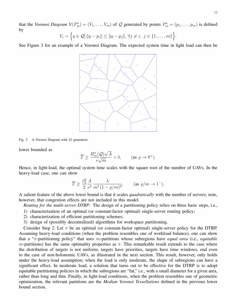
12

that the Voronoi Diagram V(P ⇤m) = (V

1

, . . . , Vm) of Q generated by points P ⇤m = (p

1

, . . . , pm) is definedby

Vi =

n

q 2 Q| kq � pik kq � pjk, 8j 6= i, j 2 {1, . . . ,m}o

.

See Figure 3 for an example of a Voronoi Diagram. The expected system time in light load can then be

Fig. 3. A Voronoi Diagram with 25 generators.

lower bounded as

T � H⇤m(Q)

pA

vpm

+ s, (as % ! 0

+

).

Hence, in light-load, the optimal system time scales with the square root of the number of UAVs. In theheavy-load case, one can show

T � �2

2

2

A

v2�

m2

(1 � %/m)

2

, (as %/m ! 1

�).

A salient feature of the above lower bound is that it scales quadratically with the number of servers; note,however, that congestion effects are not included in this model.

Routing for the multi-server DTRP: The design of a partitioning policy relies on three basic steps, i.e.,1) characterization of an optimal (or constant-factor optimal) single-server routing policy;2) characterization of efficient partitioning schemes;3) design of (possibly decentralized) algorithms for workspace partitioning.Consider Step 2. Let ⇡ be an optimal (or constant-factor optimal) single-server policy for the DTRP.

Assuming heavy-load conditions (when the problem resembles one of workload balance), one can showthat a “⇡-partitioning policy” that uses m-partitions whose subregions have equal area (i.e., equitablem-partitions) has the same optimality properties as ⇡. This remarkable result extends to the case wherethe distribution of targets is not uniform, targets have priorities, targets have time windows, end evento the case of non-holonomic UAVs, as illustrated in the next section. This result, however, only holdsunder the heavy-load assumption; when the load is only moderate, the shape of subregions can have asignificant effect. In moderate load, a solution that turns out to be effective for the DTRP is to adoptequitable partitioning policies in which the subregions are “fat,” i.e., with a small diameter for a given area,rather than long and thin. Finally, in light-load conditions, when the problem resembles one of geometricoptimization, the relevant partitions are the Median Voronoi Tessellations defined in the previous lowerbound section.

13

This discussion leads to the following (centralized) routing policy for the multi-server DTRP:

1) Compute an m median of Q, and the corresponding Voronoi partition.2) Assign one vehicle to each Voronoi region,3) Each UAV executes the single-server DTRP policy in its own subregion.

Using the above routing policy, the average system time T satisfies

T =

H⇤m(Q)

pAp

mv+ s, (as % ! 0

+

),

T �A

v2�

m2

(1 � %/m)

2

, (as m ! +1 and %/m ! 1

�).

where � is the optimality factor of the single-server routing policy.Note that the heavy-load result above relies on the fact that for large m each Voronoi region in a

Median Voronoi Tesselation has the same area (see Appendix A). For general m, this may not be thecase; furthermore, one might wonder whether equitable partitions can be computed in a decentralizedfashion (this corresponds to the third step in the aforementioned policy design procedure).

In the solution proposed in Pavone et al. (2011), Power Diagrams are the key geometric concept toobtain, in a decentralized fashion, equitable and median Voronoi partitions (or “good” approximationswhen they do not exist). Define

PW :=

⇣

(p1

, w1

), . . . , (pm, wm)

⌘

2 (Q ⇥ R)m.

The pair (pi, wi) is called a power point. The Power Diagram V(PW ) = (V1

, . . . , Vm) of Q generated bypower points PW is defined by

Vi(PW ) =

n

q 2 Q| kq � pik2 � wi kq � pjk2 � wj, 8j 6= i, j 2 {1, . . . ,m}o

.

The set PW is the set of power generators of V(PW ), and Vi is the power cell of the i-th power generator.When all weights are the same, the Power Diagram coincides with the Voronoi Diagram. One can showthat given m � 1 distinct points (p

1

, . . . , pm) in Q, there exist weights wi, i 2 {1, . . . ,m}, such that theset of power points

⇣

(p1

, w1

), . . . , (pm, wm)

⌘

generates a Power Diagram that is equitable, i.e., where allpower regions have the same area. The basic idea, then, is to associate to each UAV i a virtual powergenerator (virtual generator for short) (pi, wi); then, the power cell Vi becomes the region of dominancefor UAV i (see Figure 4). A virtual generator (pi, wi) is simply an artificial (or logical) variable whosevalue is locally controlled by the ith UAV. In general, the position of an UAV and the position of its virtualgenerator are distinct, i.e., the position of an UAV inside its own region of dominance Vi is independentfrom the position of its virtual generator (see Figure 4). Note that an equitable power diagram can beobtained by just changing the values of the weights (while keeping the generators’s positions fixed).Thus, the degrees of freedom given by the positions of the generators can be used to “steer” the partitiontoward an equitable and median Voronoi partition. Specifically, the idea is to construct an energy functionwith the properties that (1) it depends on the weights and positions of the virtual generators, and (2) allits critical points correspond to vectors of weights and positions yielding an equitable power diagram.Then, each UAV updates its own virtual generator by updating the weight according to a decentralizedgradient-descent law (with respect to the energy function) and by updating the virtual generator’s positionso as to steer the partition toward a median Voronoi diagram, when this motion does not increase thedisagreement between the areas of the neighboring regions (see Pavone et al. (2011) for details). Underthis decentralized partitioning algorithm an equitable partition is always achieved, hence the resulting

14

d2

d 1

�ta

rget

poin

tof

depa

rtur

e

�

d2

d1

�target

pointofdeparture

�

d2

d1

�targ

et

point of

depa

rture

�

d2d1

�

targetpointof departure

�

d2

d1

�target

pointofdeparture

�

Demand

Vehicle

Virtual generator(weight)

Virtual generator(position)

Region of Dominance

Fig. 4. Vehicles, virtual generators, tasks/demands and regions of dominance. A positive weight w is represented by a yellow circle withradius

pw; a negative weight w is represented by a blue circle with radius

p|w|. Note that the position of a UAV and the position of its

virtual generator are, in general, distinct.

partitioning policy is optimal in heavy load. Furthermore, if an m-median of Q that induces a Voronoipartition that is equitable exists, this partitioning algorithm will locally converge to it, thus the resultingdecentralized partitioning policy is locally optimal in light-load.

B. Multi-UAV routing with motion constraints and unlimited sensingThe definition of the problem is the same as the one for the single-server Dubins DTRP problem, but

now there are m UAVs providing service. In the following, for brevity, this problem is referred to as them-Dubins DTRP.

Lower Bounds: In contrast to the standard DTRP, the lower bound for the m-Dubins DTRP does notfollow easily from the results for the single-server Dubins DTRP. Consider first the light load case. Inthis case, the lower bound is a function of a dimensional parameter called nonholonomic vehicle density:

d⇢ :=⇢2m

A,

which is proportional to the ratio of disk whose radius is the turning radius, and the area of Q availableper vehicle. Hence, d⇢ is representative of the significance of the turning radius with respect to the typicaldistance that an individual vehicle travels. One can give the following lower bounds for the m-DubinsDTRP:

T � H⇤m(Q)

v

✓

A

m

◆

1/2

, (as � ! 0

+ and d⇢ ! 0

+

),

T � 3

3p3

4v

✓

⇢A

m

◆

1/3

, (as � ! 0

+ and d⇢ ! +1).

The first bound is obtained by approximating the Dubins distance (i.e., the length of the shortest feasiblepath for a Dubins vehicle) with the Euclidean distance. The second lower bound is obtained by explicitlytaking into account the Dubins turning cost. Note that when the motion constraint becomes “active” asd⇢ ! +1, the lower bound scales with m�1/3.

Reachability arguments show that when � is large (i.e., in heavy load), a lower bound for the heavy-load

15

Q

Fig. 5. Illustration of the the light-load policy for low values of non-holonomic density. The squares represent elements of P ⇤m(Q), the

m-median of Q. Each vehicle loiters about its respective generator at a radius ⇢. The regions of dominance are the Voronoi partition generatedby P ⇤

m(Q). In this figure, a task has appeared in the subregion roughly in the upper-right quarter of the domain. The vehicle responsiblefor this subregion has left its loitering orbit and is en route to service the demand.

case is as follows:T � 81

64

⇢A

v3�2

m3

, (as �/m ! +1).

Hence, for the m-Dubins DTRP the lower bound scales with the inverse of the cube of the number ofUAVs (in contrast to the standard DTRP where the scaling is inverse of the square); note, again, that themodel does not include congestion effects.

Routing Policies for the m-Dubins DTRP: Consider, first, the case when � is small (i.e., light load)and the non-holonomic density is low; in this case the problem resembles the standard multi-server DTRPproblem. Accordingly, the relevant partition scheme is a Median Voronoi Tesselation, and the followingpartitioning policy is efficient in this case.

1) Compute a m-median of Q,2) Assign one UAV to each Voronoi region,3) Each UAV visits the demands in the Voronoi region in the order in which they arrive. When

no demands are available, the UAV returns to the median and loiters on a circular trajectory ofradius ⇢ centered at the median of the subregion.

This policy is illustrated in Figure 5. The performance of this policy is given by

T H⇤m(Q)

v

✓

A

m

◆

1/2

, (as � ! 0

+ and d⇢ ! 0

+

),

i.e., this policy is optimal. Hence, in this asymptotic regime the system time scales as 1/(vpm).

In light-load, when the non-holonomic density is large, one should instead consider dynamic partitions;in particular, an effective policy is as follows:

1) Bound the environment Q with a rectangle of minimum height, where height denotes the smallerof the two side lengths of a rectangle. Let W and H be the width and height of this boundingrectangle, respectively. Divide Q into strips of width w, where

w = min

n⇣

4

3

p⇢

WH + 10.38⇢H

m

⌘

2/3

, 2⇢o

.

16

2) Orient the strips along the side of length W .3) Construct a closed Dubins path which runs along the longitudinal bisector of each strip, visiting

all strips in top-to-bottom sequence, making U-turns between strips at the edges of Q, and finallyreturning to the initial configuration. The m UAVs loiter on this path, equally spaced, in termsof path length.

A depiction of this policy is shown in Figure 6. At the instant a target arrives, one constructs a circle ofradius ⇢ which is tangent to the loitering path and intersects the target. The UAV responsible for visitingthe target is the one closest in terms of loitering path length to the point of departure, at the time oftarget-arrival. After a UAV has serviced a target, it must return to its place in the loitering pattern.

Q

Fig. 6. Illustration of the the light-load policy for large non-holonomic densities. The segment providing closure of the loitering path(returning the UAVs from the end of the last strip to the beginning of the first strip) is not shown here for clarity of the drawing.

Note that the dynamic partition associated with a particular UAV is in fact fixed in the reference frameof that UAV and that in the global frame these partitions could be regarded as a dynamic version of anequitable partition of Q, modulo the boundary effects. The reason for using dynamic equitable partitionsis as follows. For large values of non-holonomic density, the area per vehicle is small in comparison to thedisk of radius ⇢, and hence the efficient regions of responsibility for the UAVs in such a regime coincidewith their small-time reachable sets. Since the UAVs modeled as a Dubins vehicle can not stall, a simpleway to ensure that the regions of responsibility are contained inside the small-time reachable sets all thetime is to have the regions of responsibility fixed in the reference frame of the UAVs.

The system time of the above policy that uses dynamic partitions satisfies

T

8

<

:

1.238v

⇣

⇢WH+10.38⇢2Hm

⌘

1/3

+

W+H+6.19⇢mv

for m � 0.471⇣

WH⇢2

+

10.38H⇢

⌘

,WH+10.38⇢H

4⇢mv+

W+H+6.19⇢mv

+

1.06⇢v

otherwise.

Hence this policy is within a constant factor of the optimal in the asymptotic regime where �/m ! 0

+

and d⇢ ! +1. Moreover, in such asymptotic regime the optimal system time scales as 1/(v 3pm).

Finally, for the heavy load, the relevant partitions are additively-weighted equitable partitions, as follows:

1) Divide the environment into regions of dominance with lines parallel to the bead rows. Let thearea and height of the ith vehicle’s region be denoted with Ai and Hi. Place the subregiondividers in such a way that

Ai +7

3

⇡⇢Hi =1

m

✓

A+

7

3

⇡⇢H

◆

, for all i 2 {1, . . . ,m}.

2) Allocate one subregion to every vehicle.

17

3) Each vehicle executes the single vehicle policy in its own region, where the size of bead inregion i is chosen to be `i = min{C

BT,iv/�i, 4⇢}, with �i = �Ai/A being the arrival rate in

region i, and CBT,i =

7�p17

4

⇣

1 +

7⇡⇢Hi

3Ai

⌘�1

.

The system time for this policy satisfies

T 71

⇢A

v3

✓

1 +

7⇡⇢H

3A

◆

3

�2

m3

, (as �/m ! +1).

Hence this policy is within a constant factor of the optimal in heavy-load, and that the optimal systemtime in this case scales as �2/(mv)3.

Note that all the three above policies are partitioning policies; the partitions used are, however, quite dif-ferent, ranging from Median Voronoi Tesselations, to dynamic partitions, to additively-weighted equitablepartitions. Median Voronoi Tesselations and additively-weighted equitable partitions can be computed ina decentralized fashion with the partitioning algorithm discussed for the multi-DTRP problem (indeed, aMedian Voronoi Tesselation can be computed even without inter-agent communication). No decentralizedalgorithms have been developed so far for dynamic partitions.

It is instructive to compare the scaling of the optimal system time with respect to �, m and v forthe m-DTRP and for the m-Dubins DTRP. Such comparison is shown in Table I. One can observe that

TABLE IA COMPARISON BETWEEN THE SCALING OF THE OPTIMAL SYSTEM TIME FOR THE MULTI-SERVER DTRP AND FOR THE m-DUBINS

DTRP.

T⇤, m-DTRP T

⇤, m-Dubins DTRP

Heavy load(�/m ! +1)

⇥

✓

�

m2v2

◆

⇥

✓

�2

m3v3

◆

Light load(�/m ! 0

+)⇥

✓

1

vpm

◆

⇥

✓

1

vpm

◆

if d⇢ ! 0

+

⇥

✓

1

v 3pm

◆

if d⇢ ! +1

in heavy-load the optimal system time for the m-Dubins DTRP is of the order �2/(mv)3, whereas forthe m-DTRP it is of the order �/(mv)2. This analysis rigorously establishes the following intuitive fact:bounded-curvature constraints make the optimal system much more sensitive to increases in the demandgeneration rate. Perhaps less intuitive is the fact that the optimal system time is also more sensitive withrespect to the number of vehicles and the vehicle speed in the m-Dubins DTRP as compared to them-DTRP. In the light load, the optimal system time for the m-DTRP is of the order 1/(v

pm), which is

the same for the m-DTRP but only when the non-holonomic density is small. When the non-holonomicdensity is high, the optimal system time is of the order 1/(v 3

pm), i.e., it is more sensitive to the number

of vehicles than in the low non-holonomic density case. This suggests the existence of a critical value ofd⇢ below which the partitioning policy using Median Voronoi partitions is efficient, and above which the

18

partitioning policy that uses dynamic partitions is efficient. The details of such phase transitions can befound in Enright et al. (2009).

C. Multi-UAV Routing with Limited Sensing CapabilitiesThe definition of the problem is the same as in the single-server Persistent Patrolling Problem, with

the only difference being the number of UAVs providing service.Lower Bounds: As in the single-server case, the discussion will focus on the case in which � ! 0

+.In this case the system time is bounded by

T � 1

4mv�

✓

Z

Q

p

'(q) dq

◆

2

+ s.

Routing policies for the m-server PPP: Optimal static partitioning policies can be designed usingpartitions that are simultaneously equitable with respect to ' and to p

'. (Such partitions can always befound.) However, a simpler strategy is based on a “dynamic” partition, as follows:

1) If any outstanding tasks have been revealed, use the multi-server DTRP routing policy tocomplete these tasks.

2) Otherwise, move to the “next” tile in the “next” subregion, and sweep this tile using a lawnmowerpattern. (The initial tile and subregion for each vehicle are chosen in such a way that vehiclesare uniformly spaced along the sub-region/tile cycle.)

3) Repeat.

The above policy matches the lower bound, and is hence optimal as � ! 0

+. In the case in which� is finite, and % ! 1

�, the sensing-range limitation does not constrain the system’s performance, andthe performance for the “standard” multi-server DTRP is recovered. As discussed above, no decentralizedalgorithms have been developed so far for dynamic partitions.

V. CONCLUSIONS

In this chapter, we presented a dynamic vehicle routing framework for coordination of UAVs performingspatially distributed tasks in uncertain and dynamic environments. The technical approach relies onusing algorithmic spatial queueing theory for designing efficient algorithms for single vehicles, andthen augmenting it with spatial partitioning policies to extend it to multiple vehicles. To illustrate thisapproach, a variety of problems were considered, ranging from the simplest case with no motion orsensing constraints, to the cases with motion differential constraints and with limited sensing constraints.Additionally, multi-UAV versions for each of these cases were considered. For each scenario, UAV routingpolicies have been provided, which are provably optimal or approximately optimal in the asymptoticregimes of light and heavy load. The dependence of the performance of these algorithms on missionparameters such as the number, speed, sensor footprint and turning radius of the UAVs, and the dimensionof the workspace was discussed. A system designer could interpolate between such scaling laws for theextreme cases as established in this chapter, to choose a policy that best fits given problem specifications.Moreover, the algorithms and their underlying principles presented in this chapter for canonical scenarioscould also provide guidelines to design algorithms for other scenarios not explicitly considered in thischapter.

REFERENCESP. K. Agarwal and M. Sharir. Efficient algorithms for geometric optimization. ACM Computing Surveys, 30(4):412–458, 1998.M. Alighanbari and J. P. How. A robust approach to the UAV task assignment problem. International Journal on Robust and

Nonlinear Control, 18(2):118–134, 2008.

19

D. Applegate, R. Bixby, V. Chvatal, and W. Cook. On the solution of traveling salesman problems. In Documenta Mathematica,Journal der Deutschen Mathematiker-Vereinigung, pages 645–656, Berlin, Germany, 1998. Proceedings of the InternationalCongress of Mathematicians, Extra Volume ICM III.

S. Arora. Nearly linear time approximation scheme for Euclidean TSP and other geometric problems. In Proc. 38th IEEEAnnual Symposium on Foundations of Computer Science, pages 554–563, 1997.

G. Arslan, J. R. Marden, and J. S. Shamma. Autonomous vehicle-target assignment: A game theoretic formulation. ASMEJournal on Dynamic Systems, Measurement, and Control, 129(5):584–596, 2007.

R. W. Beard, T. W. McLain, M. A. Goodrich, and E. P. Anderson. Coordinated target assignment and intercept for unmannedair vehicles. IEEE Trans. on Robotics and Automation, 18(6):911–922, 2002.

J. Beardwood, J. Halton, and J. Hammersley. The shortest path through many points. Proceedings of the Cambridge PhiloshopySociety (Mathematical and Physical Sciences), 55(4):299–327, 1959.

D. J. Bertsimas and G. J. van Ryzin. A stochastic and dynamic vehicle routing problem in the Euclidean plane. OperationsResearch, 39:601–615, 1991.

D. J. Bertsimas and G. J. van Ryzin. Stochastic and dynamic vehicle routing in the Euclidean plane with multiple capacitatedvehicles. Operations Research, 41(1):60–76, 1993a.

D. J. Bertsimas and G. J. van Ryzin. Stochastic and dynamic vehicle routing with general interarrival and service timedistributions. Advances in Applied Probability, 25:947–978, 1993b.

F. Bullo, E. Frazzoli, M. Pavone, K. Savla, and S.L. Smith. Dynamic vehicle routing for robotic systems. Proceedings of theIEEE, 99(9):1482 –1504, 2011.

G. Cannata and A. Sgorbissa. A minimalist algorithm for multirobot continuous coverage. IEEE Trans. on Robotics, 27(2),2011.

P. Chandler, S. Rasmussen, and M. Pachter. UAV cooperative path planning. In AIAA Conf. on Guidance, Navigation, andControl, 2000.

N. Christofides. Bounds for the travelling-salesman problem. Operations Research, 20:1044–1056, 1972.Z. Drezner, editor. Facility Location: A Survey of Applications and Methods. Series in Operations Research. Springer, 1995.

ISBN 0-387-94545-8.L.E. Dubins. On curves of minimal length with a constraint on average curvature and with prescribed initial and terminal

positions and tangents. American Journal of Mathematics, 79:497–516, 1957.J. J. Enright, K. Savla, E. Frazzoli, and F. Bullo. Stochastic and dynamic routing problems for multiple UAVs. AIAA J. of

Guidance, Control, and Dynamics, 32(4):1152–1166, 2009.B. Golden, S. Raghavan, and E. Wasil. The Vehicle Routing Problem: Latest Advances and New Challenges, volume 43 of

Operations Research/Computer Science Interfaces. Springer, 2008. ISBN 0387777776.S. Irani, X. Lu, and A. Regan. On-line algorithms for the dynamic traveling repair problem. Journal of Scheduling, 7(3):

243–258, 2004.P. Jaillet and M. R. Wagner. Online routing problems: Value of advanced information and improved competitive ratios.

Transportation Science, 40(2):200–210, 2006.D. S. Johnson, L. A. McGeoch, and E. E. Rothberg. Asymptotic experimental analysis for the held-karp traveling salesman

bound. In Proc. 7th Annual ACM-SIAM Symposium on Discrete Algorithms, pages 341–350, 1996.S. O. Krumke, W. E. de Paepe, D. Poensgen, and L. Stougie. News from the online traveling repairman. Theoretical Computer

Science, 295(1-3):279–294, 2003.R. Larson and A. Odoni. Urban Operations Research. Prentice Hall, Englewood Cliffs, NJ, 1981.S. Lin and B. W. Kernighan. An effective heuristic algorithm for the traveling-salesman problem. Operations Research, 21:

498–516, 1973.J. D. C. Little. A Proof for the Queuing Formula: L= �W. Operations Research, 9(3):pp. 383–387, 1961. ISSN 0030364X.

URL http://www.jstor.org/stable/167570.G. Mathew and I. Mezic. Spectral multiscale coverage: A uniform coverage algorithm for mobile sensor networks. In

Proceedings of the 48th IEEE Control and Decision Conference, pages 7872–7877, Shanghai, China, December 2009.N. Megiddo and K. J. Supowit. On the complexity of some common geometric location problems. SIAM Journal on Computing,

13(1):182–196, 1984. ISSN 0097-5397.A.R. Mesquita. Exploiting Stochasticity in Multi-agent Systems. PhD thesis, University of California at Santa Barbara, Santa

Barbara, CA, 2010.B. J. Moore and K. M. Passino. Distributed task assignment for mobile agents. IEEE Transactions on Automatic Control, 52

(4):749–753, 2007.C. H. Papadimitriou. Worst-case and probabilistic analysis of a geometric location problem. SIAM Journal on Computing, 10

(3), August 1981.M. Pavone. Dynamic Vehicle Routing for Robotic Networks. PhD thesis, Department of Aeronautics and Astronautics,

Massachusetts Institute of Technology, June 2010.

20

M. Pavone, K. Savla, and E. Frazzoli. Sharing the load. IEEE Robotics and Automation Magazine, 16(2):52–61, 2009.M. Pavone, A. Arsie, E. Frazzoli, and F. Bullo. Distributed algorithms for environment partitioning in mobile robotic networks.

IEEE Trans. on Automatic Control, 56(8):1834–1848, 2011.G. Percus and O. C. Martin. Finite size and dimensional dependence of the Euclidean traveling salesman problem. Physical

Review Letters, 76(8):1188–1191, 1996.H. N. Psaraftis. Dynamic programming solution to the single vehicle many-to-many immediate request dial-a-ride problem.

Transportation Science, 14(2):130–154, 1980.D. D. Sleator and R. E. Tarjan. Amortized efficiency of list update and paging rules. Communications of the ACM, 28(2):

202–208, 1985.S. L. Smith and F. Bullo. Monotonic target assignment for robotic networks. IEEE Trans. on Automatic Control, 54(9):

2042–2057, 2009.D. Song, C. Y. Kim, and J. Yi. Stochastic modeling of the expected time to search for an intermittent signal source under a

limited sensing range. In Proceedings of Robotics: Science and Systems, Zaragoza, Spain, June 2010.J. M. Steele. Probabilistic and worst case analyses of classical problems of combinatorial optimization in Euclidean space.

Mathematics of Operations Research, 15(4):749, 1990.L.D. Stone. Theory of Optimal Search. Academic Press, New York, NY, 1975.P. Toth and D. Vigo, editors. The Vehicle Routing Problem. Monographs on Discrete Mathematics and Applications. SIAM,

2001. ISBN 0898715792.P. Van Hentenryck, R. Bent, and E. Upfal. Online stochastic optimization under time constraints. Annals of Operations

Research, 177(1):151–183, 2009.Eitan Zemel. Probabilistic analysis of geometric location problems. Annals of Operations Research, 1(3), October 1984.

APPENDIX

A. The continuous multi-median problemGiven a set Q ⇢ Rd and a vector P = (p

1

, . . . , pm) of m distinct points in Q, the expected distancebetween a random point q, generated according to a probability density function ', and the closest pointin P is given by

Hm(P,Q) := E

min

i2{1,...,m}kpi � qk

�

=

mX

i=1

Z

Vi(P,Q)

kpi � qk'(q)dq,

where V(P,Q) = (V1

(P,Q), . . . ,Vm(P,Q) is the Voronoi partition of the set Q generated by the pointsP . In other words, q 2 Vi(P,Q) if kq�pik kq�pkk, for all k 2 {1, . . . ,m}. The set Vi is referred to asthe Voronoi cell of the generator pi. The function Hm is known in the locational optimization literature asthe continuous Weber function or the continuous multi-median function; see (Agarwal and Sharir, 1998;Drezner, 1995) and references therein.

The m-median of the set Q, with respect to the measure induced by ', is the global minimizer

P ⇤m(Q) = argmin

P2QmHm(P,Q).

Let H⇤m(Q) = Hm(P

⇤m(Q),Q) be the global minimum of Hm. It is straightforward to show that the map

P 7! H1

(P,Q) is differentiable and strictly convex on Q. Therefore, it is a simple computational taskto compute P ⇤

1

(Q). It is convenient to refer to P ⇤1

(Q) as the median of Q. On the other hand, the mapP 7! Hm(P,Q) is differentiable (whenever (p

1

, . . . , pm) are distinct) but not convex, thus making thesolution of the continuous m-median problem hard in the general case. It is known (Agarwal and Sharir,1998; Megiddo and Supowit, 1984) that the discrete version of the m-median problem is NP-hard ford � 2. Gradient algorithms for the continuous m-median problems can be designed by means of theequality

@Hm(P,Q)

@pi=

Z

Vi(P,Q)

pi � q

kpi � qk '(q)dq.

21

The set of critical points of Hm contains all configurations (p1

, . . . , pm) with the property that each pi isthe generator of the Voronoi cell Vi(P,Q) as well as the median of Vi(P,Q). We refer to such Voronoidiagrams as median Voronoi diagrams. It is possible to show that a median Voronoi diagram always existsfor any bounded convex domain Q and density '.

The dependence of H⇤m(Q) on m plays a crucial role in the design and analysis of algorithms relying

on geometric optimization. However, finding the exact relationship for the general case is difficult; hence,it is of great interest to provide bounds on H⇤

m(Q). This problem is studied thoroughly in Papadimitriou(1981) for square regions and in Zemel (1984) for more general compact regions. It is known that, in theasymptotic case (m ! +1), H⇤

m(Q) = chex

p

A/m almost surely, where chex

⇡ 0.377 is the first momentof a hexagon of unit area about its center. This optimal asymptotic value is achieved by placing the mpoints at the centers of the hexagons in a regular hexagonal lattice within Q (the honeycomb heuristic).Working towards the above result, it is also known that for any m 2 N:

2

3

r

A

⇡m H⇤

m(Q) c(Q)

r

A

m,

where c(Q) is a constant depending on the shape of Q.

B. The Euclidean Traveling Salesman ProblemThe Euclidean TSP is formulated as follows: given a finite set D of n points in Rd, find the minimum-

length closed curve through all points in D. In graph theoretical language, a tour of the point set D is aspanning cycle of the complete graph with vertex set P ; the length of a tour is the sum of all Euclideandistances between points in the tour.

The asymptotic behavior of stochastic TSP problems for large n exhibits the following interestingproperty. Let ETSP(n) be a random variable returning the length of the Euclidean TSP tour through npoints, independently and uniformly sampled from a compact set Q of unit area; in Beardwood et al.(1959) it is shown that there exists a constant �

2

such that, almost surely,

lim

n!+1

ETSP(n)pn

= �2

.

In other words, the optimal cost of stochastic TSP tours approaches a deterministic limit, and grows asthe square root of the number of points to be visited; the current best estimate of the constant appearingin the limit is �

2

= 0.7120± 0.0002, see Johnson et al. (1996); Percus and Martin (1996). Similar resultshold in higher dimensions, and for non-uniform point distributions: from Steele (1990), the limit (B) takesthe general form

lim

n!+1

ETSP(n)

n1�1/d= �d

Z

Q'(q)1�1/d dq almost surely,

where ' is the density of the absolutely continuous part of the distribution ' from which the n pointsare independently sampled. Notice that the bound holds for all compact sets: the shape of the set onlyaffects the convergence rate to the limit. According to Larson and Odoni (1981), if Q is a “fairly compactand fairly convex” set in the plane, the estimate ETSP(n) ⇡ �

2

pn for values of n as low as 15.

Remarkably, the asymptotic cost of the stochastic TSP for uniform point distributions is an upper boundon the asymptotic cost for general point distributions, i.e.,

lim

n!+1

ETSP(n)

n1�1/d �d.

This follows directly from an application of Jensen’s inequality, i.e.,Z

Q'(q)1�

1d dq

✓

Z

Q'(q) dq

◆

1� 1d

'(Q)

1� 1d= 1.

22

The TSP is known to be NP-hard, which suggests that there is no general algorithm capable of findingthe optimum tour in an amount of time polynomial in the size of the input. Even though the exact optimalsolutions of a large TSP can be very hard to compute, several exact and heuristic algorithms and softwaretools are available for the numerical solution of Euclidean TSPs.

The most advanced TSP solver to date is arguably concorde (Applegate et al., 1998). Heuristicpolynomial-time algorithms are available for constant-factor approximations of TSP solutions, such asChristofides’ algorithm, providing a 3/2 approximation factor (Christofides, 1972). On a more theoreticalside, Arora (1997) proved the existence of polynomial-time approximation schemes, providing a (1 + ")constant-factor approximation for any " > 0.

A modified version of the Lin-Kernighan heuristic (Lin and Kernighan, 1973) is implemented inlinkern; this powerful solver yields approximations in the order of 5% of the optimal tour cost veryquickly for many instances. For example, in numerical experiments on a 2.4 GHz Pentium machine,approximations of random TSPs with 1,000 points typically required about two seconds of CPU time.Both concorde and linkern are written in ANSI C and, at the time of writing, are freely availablefor academic research use at http://www.tsp.gatech.edu/concorde/index.html.

In this chapter, several routing policies were presented requiring on-line solutions of large TSPs. Prac-tical implementations of the algorithms will rely on heuristics, such as Lin-Kernighan’s or Christofides’.If a constant-factor approximation algorithm is used, the effect on the asymptotic performance guaranteesof our algorithms can be simply modeled as a scaling of the constant �d.