
1 Theoretical background - California Institute of...
23
Lecture notes: Auction models 1 Papers to be covered: • Laffont, Ossard, and Vuong (1995) • Guerre, Perrigne, and Vuong (2000) • Haile, Hong, and Shum (2003) In this lecture, focus on empirical of auction models. Auctions are models of asymmetric information which have generated the most interest empirically. We begin by summarizing some relevant theory. 1 Theoretical background An auction is a game of incomplete information. Assume that there are N players, or bidders, indexed by i =1,... ,N . There are two fundamental random elements in any auction model. • Bidders’ private signals X 1 ,... ,X N . We assume that the signals are scalar random variables, although there has been recent interest in models where each signal is multi- dimensional. • Bidders’ utilities: u i (X i ,X −i ), where X −i ≡{X 1 ,... ,X i−1 ,X i+1 ,... ,X N }, the vec- tor of signals excluding bidder i’s signal. Since signals are private, V i ≡ u i (X i ,X −i ) is a random variable from all bidders’ point of view. In what follows, we will also refer to bidder i’s (random) utility as her valuation. Differing assumptions on the form of bidders’ utility function lead to the important dis- tinction between common value and private value models. In the private value case, V i = X i , ∀i: each bidder knows his own valuation, but not that of his rivals. 1 In the (pure) common value case, V i = V, ∀i, where V is in turn a random variable from all bidders’ point of view, and bidders’ signals are to be interpreted as their noisy estimates of the true but known common value V . Therefore, signals will generally not be independent when com- mon values are involved. More generally a common value model arises when u i (X i ,X −i ) is functionally dependent on X −i . 1 More generally, in a private value model, ui (Xi ,X−i ) is restricted to be a function only of Xi . 1
Transcript of 1 Theoretical background - California Institute of...

Lecture notes: Auction models 1
Papers to be covered:
• Laffont, Ossard, and Vuong (1995)
• Guerre, Perrigne, and Vuong (2000)
• Haile, Hong, and Shum (2003)
In this lecture, focus on empirical of auction models. Auctions are models of asymmetric
information which have generated the most interest empirically. We begin by summarizing
some relevant theory.
1 Theoretical background
An auction is a game of incomplete information. Assume that there are N players, or
bidders, indexed by i = 1, . . . , N . There are two fundamental random elements in any
auction model.
• Bidders’ private signals X1, . . . ,XN . We assume that the signals are scalar random
variables, although there has been recent interest in models where each signal is multi-
dimensional.
• Bidders’ utilities: ui (Xi,X−i), where X−i ≡ {X1, . . . ,Xi−1,Xi+1, . . . ,XN}, the vec-
tor of signals excluding bidder i’s signal. Since signals are private, Vi ≡ ui(Xi,X−i) is
a random variable from all bidders’ point of view. In what follows, we will also refer
to bidder i’s (random) utility as her valuation.
Differing assumptions on the form of bidders’ utility function lead to the important dis-
tinction between common value and private value models. In the private value case,
Vi = Xi, ∀i: each bidder knows his own valuation, but not that of his rivals.1 In the (pure)
common value case, Vi = V, ∀i, where V is in turn a random variable from all bidders’ point
of view, and bidders’ signals are to be interpreted as their noisy estimates of the true but
known common value V . Therefore, signals will generally not be independent when com-
mon values are involved. More generally a common value model arises when ui(Xi,X−i) is
functionally dependent on X−i.
1More generally, in a private value model, ui(Xi, X−i) is restricted to be a function only of Xi.
1

Lecture notes: Auction models 2
Before proceeding, we give some examples to illustrate the auction formats discussed above.
• Symmetric independent private values (IPV) model: Xi ∼ F , i.i.d. across all bid-
ders i, and Vi = Xi. Therefore, F (X1, . . . ,XN ) = F (X1) ∗ F (X2) · · · ∗ F (XN ), and
F (V1,X1, . . . , VN ,XN ) =∏
i [F (Xi)]2.
• Conditional independent model: signals are independent, conditional on a common
component V . Vi = V,∀i, but F (V,X1, . . . ,XN ) = F (V )∏
i F (Xi|V ).
Models also differ depending on the auction rules. In a first-price auction, the object
is awarded to the highest bidder, at her bid. A second-price auction also awards the
object to the highest bidder, but she pays a price equal to the bid of the second-highest
bidder. (Sometimes second-price auctions are also called “Vickrey” auctions, after the late
Nobel laureate William Vickrey.) In an English or ascending auction, the price the raised
continuously by the auctioneer, and the winner is the last bidder to remain, and he pays an
amount equal to the price at which all of his rivals have dropped out of the auction. In a
Dutch auction, the price is lowered continuously by the auctioneer, and the winner is the
first bidder to agree to pay any price.
There is a large amount of theory and empirical work. In this lecture, we focus on first-
price auction models. We also discuss a few theoretical concepts that will come up in the
empirical papers discussed later.
1.1 Equilibrium bidding
In discussing equilibrium bidding in the different auction models, we will focus on the general
symmetric affiliated model, used in the seminal paper of Milgrom and Weber (1982). The
assumptions made in this model are:
• Vi = ui(Xi,X−i)
• Symmetry: F (V1,X1, . . . , VN ,XN ) is symmetric (i.e., exchangeable) in the indices i
so that, for example, F (VN ,XN , . . . , V1,X1) = F (V1,X1, . . . , VN ,XN ).
• The random variables V1, . . . , VN ,X1, . . . ,XN are affiliated. Let Z1, . . . , ZM and
Z∗1 , . . . , Z∗
M denote two realizations of a random vector process, and Z and Z de-
note, respectively, the component-wise maximum and minimum. Then we say that
2

Lecture notes: Auction models 3
Z1, . . . , ZM are affiliated if F (Z)F (Z) ≥ F (Z1, . . . , ZM )F (Z∗1 , . . . , Z∗
M ). In other
words, large values for some of the variables make large values for the other variables
most likely. Affiliation implies useful stochastic orderings on the conditional distri-
butions of bidders’ signals and valuations, which is necessary in deriving monotonic
equilibrium bidding strategies.
Let Yi ≡ maxj 6=i Xj , the highest of the signals observed by bidder i’s rivals. Given affiliation,
the conditional expectation E[Vi|Xi, Yi] is increasing in both Xi and Yi.
Winner’s curse Another consequence of affiliation is the winner’s curse, which is just
the fact that
E[Vi|Xi] ≥ E[Vi|Xi > Yi]
where the conditioning event in the second expectation (Xi > Yi) is the event of winning
the auction.
To see this, note that
E[Vi|Xi] = EX−iE [Vi|Xi;X−i] =
∫
· · ·
∫
︸ ︷︷ ︸
N−1
E [Vi|Xi;X−i]F (dX1, . . . , dXN )
≥
∫ Xi
· · ·
∫ Xi
︸ ︷︷ ︸
N−1
E [Vi|Xi;X−i]F (dX1, . . . , dXN )
= E [Vi|Xi > Xj , j 6= i] = E [Vi|Xi > Yi] .
In other words, if bidder i “naively” bids E [Vi|Xi], her expected payoff from a first-price
auction is negative for every Xi. In equilibrium, therefore, rational bidders should “shade
down” their bids by a factor to account for the winner’s curse.
This winner’s curse intuition arises in many non-auction settings also. For example, in
two-sided markets where traders have private signals about unknown fundamental value of
the asset, the ability to consummate a trade is “good news” for sellers, but “bad news” for
buyers, implying that, without ex-ante gains from trade, traders may not be able to settle
on a market-clearing price. The result is the famous “lemons” result by Akerlof (1970), as
well as a version of the “no-trade” theorem in Milgrom and Stokey (1982). Glosten and
Milgrom (1985) apply the same intuition to explain bid-ask spreads in financial markets.
3

Lecture notes: Auction models 4
Next, we cover some specific auction results in some detail, in order to understand method-
ology in the empirical papers.
1.2 First-price auctions
We derive the symmetric monotonic equilibrium bidding strategy b∗(·) for first-price auc-
tions. If bidder i wins the auction, he pays his bid b∗(Xi). His expected profit is
=E [(Vi − b)1 (b∗(Yi) < b) |Xi = x]
=EYiE[
(Vi − b)1(
Yi < b∗−1(b))
|Xi = x, Yi
]
=EYi
[
(V (x, Yi) − b)1(
Yi < b∗−1(b))
|Xi = x]
=
∫ b∗−1(b)
−∞(V (x, Yi) − b)f(Yi|x)dYi.
The first-order conditions are
0 = −
∫ b∗−1(b)
−∞f(Yi|x)dYi +
1
b∗′(x)
[(V (x, x) − b) ∗ fYi|Xi
(x|x)]⇔
0 = − FYi|x(x|x) +1
b∗′(x)
[(V (x, x) − b) ∗ fYi|Xi
(x|x)]⇔
b∗′(x) = (V (x, x) − b∗(x))
[f(x|x)
F (x|x)
]
⇒
b∗(x) = exp
(
−
∫ x
x
f(s|s)
F (s|s)ds
)
b(x) +
∫ x
x
V (α,α)dL(α|x)
where
L(α|x) = exp
(
−
∫ x
α
f(s|s)
F (s|s)
)
.
Initial condition: b(x) = V (x, x).
For the IPV case:
V (α,α) = α
F (s|s) = F (s)N−1
f(s|s) = (n − 1)F (s)N−2f(s)
4

Lecture notes: Auction models 5
An example Xi ∼ U [0, 1], i.i.d. across bidders i. Then F (s) = s, f(s) = 1. Then
b∗(x) = 0 +
∫ x
0α exp
(
−
∫ x
α
(n − 1)f(s)
sF (s)ds
)(n − 1)f(α)
αF (α)dα
=
∫ x
0exp
(
−(n − 1)(logx
α))
(n − 1)dα
=
∫ x
0
(α
x
)N−1(N − 1)dα
= α
(N − 1
N
)(α
x
)N]x
0
=
(N − 1
N
)
x.
1.2.1 Reserve prices
A reserve price just changes the initial condition of the equilibrium bid function. With
reserve price r, initial condition is now b(x∗(r)) = r. Here x∗(r) denotes the screening
value, defined as
x∗(r) ≡ inf {x : E [Vi|Xi = x, Yi < x] ≥ r} . (1)
Conditional expectation in brackets is value of winning to bidder i, who has signal x.
Screening value is lowest signal such that bidder i is willing to pay at least the reserve price
r.
(Note: in PV case, x∗(r) = r. In CV case, with affiliation, generally x∗(r) > r, due to
winners curse.)
Equilibrium bidding strategy is now:
b∗(x)
{
= exp(
−∫ x
x∗(r)f(s|s)F (s|s)ds
)
r +∫ x
x∗(r) V (α,α)dL(α|x) for x ≥ x∗(r)
< r for x < x∗(r)
For IPV, uniform example above:
b∗(x) =
(N − 1
N
)
x +1
N
( r
x
)N−1r.
1.3 Second-price auctions
Assume the existence of a monotonic equilibrium bidding strategy b∗(x). Next we derive
the functional form of this equilibrium strategy.
5

Lecture notes: Auction models 6
Given monotonicity, the price that bidder i will pay (if he wins) is b∗(Yi): the bid submitted
by his closest rivals. He only wins when his bid b < b∗(Yi). Therefore, his expected profit
from participating in the auction with a bid b and a signal Xi = x is:
EYi[(Vi − b∗(Yi))1 (b∗(Yi) < b) |Xi = x]
=EYi[(Vi − b∗(Yi))1 (Yi < Xi) |Xi = x]
=EYi|XiE [(Vi − b∗(Yi))1 (Yi < Xi) |Xi = x, Yi]
=EYi|Xi[(E(Vi|Xi, Yi) − b∗(Yi))1 (Yi < Xi)]
≡EYi|Xi[(v(Xi, Yi) − b∗(Yi))1 (Yi < Xi)]
=
∫ (b∗)−1(b)
−∞(v(x, Yi) − b∗(Yi)) f (Yi|Xi = x) .
(2)
Bidder i chooses his bid b to maximize his profits. The first-order conditions are (using
Leibniz’ rule):
0 = b∗−1′(b) ∗[
v(x, b∗−1(b)) − b∗(b∗−1(b))]
∗ f(b∗−1(b)|Xi) ⇔
0 =1
b∗′(b)[v(x, x) − b∗(x)] ∗ f(b∗−1(b)|Xi) ⇔
b∗(x) = v(x, x) = E [Vi|Xi = x, Yi = x] .
In the PV case, the equilibrium bidding strategy simplifies to
b∗(x) = v(x, x) = x.
With reserve price, equilibrium strategy remains the same, except that bidders with signals
less than the screening value x∗(r) (defined in Eq. (1) above) do not bid.
2 Laffont-Ossard-Vuong (1995): “Econometrics of First-Price
Auctions”
• Structural estimation of 1PA model, in IPV context.
• Example of a parametric approach to estimation.
• Goal of empirical work:
– We observe bids b1, . . . , bn, and we want to recover valuations v1, . . . , vn.
6

Lecture notes: Auction models 7
– Why? Analogously to demand estimation, we can evaluate the “market power”
of bidders, as measured by the margin v − p.
Could be interesting to examine: how fast does margin decrease as n (number
of bidders) increases?
– Useful for the optimal design of auctions:
1. What is auction format which would maximize seller revenue?
2. What value for reserve price would maximize seller revenue?
• Another exercise in simulation estimation
���
MODEL
• I bidders
• Information structure is IPV: valuations vi, i = 1, . . . , I are i.i.d. from F (·|zl, θ) where
l indexes auctions, and zl are characteristics of l-th auctions
• θ is parameter vector of interest, and goal of estimation
• p0 denotes “reserve price”: bid is rejected if < p0.
• Dutch auction: strategically identical to first-price sealed bid auction.
Equilibrium bidding strategy is:
bi = e(vi, I, p0, F
)=
vi −
R vi
p0 F (x)I−1dx
F (vi)I−1 if vi > p0
0 otherwise(3)
Note: (1) bi(vi = p0) = p0; (2) strictly increasing in vi.
���
Dataset: only observe winning bid bwl for each auction l. Because bidders with lower bids
never have a chance to bid in Dutch auction.
Given monotonicity, the winning bid bw = e(v(I), I, p0, F
), where v(I) ≡ maxi vi (the highest
order statistic out of the I valuations).
7

Lecture notes: Auction models 8
Furthermore, the CDF of v(I) is F (·|zl, θ)I , with corresponding density I · F I−1f .
���
Goal is to estimate θ by (roughly speaking) matching the winning bid in each auction l to
its expectation.
Expected winning bid is (for simplicity, drop zl and θ now)
Ev(I)>p0(bw) =
∫ ∞
p0
e(v(I), I, p0, F
)I · F (v|θ)I−1f(v|θ)dv
= I
∫ ∞
p0
(
v −
∫ v
p0 F (x)I−1dx
F (v)I−1
)
F (v|θ)I−1f(v|θ)dv
= I
∫ ∞
p0
(
v · F (v)I−1 −
∫ ∞
p0
F (x)I−1dx
)
f(v)dv. (∗).
���
If we were to estimate by simulated nonlinear least squares, we would proceed by finding
θ to minimize the sum-of-squares between the observed winning bids and the predicted
winning bid, given by expression (*) above. Since (*) involves complicated integrals, we
would simulate (*), for each parameter vector θ.
How would this be done:
• Draw valuations vs, s = 1, . . . , S i.i.d. according to f(v|θ). This can be done by
drawint u1, . . . , uS i.i.d. from the U [0, 1] distribution, then transform each draw:
vs = F−1(us|θ).
• For each simulated valuation vs, compute integrand Vs = vsF (vs|θ)I−1−∫ vs
p0 F (x|θ)I−1dx.
(Second term can also be simulated, but one-dimensional integral is that very hard to
compute.)
• Approximate the expected winning bid as 1S
∑
s Vs.
However, the authors do not do this— they propose a more elegant solution. In particular,
they simplify the simulation procedure for the expected winning bid by appealing to the
Revenue-Equivalence Theorem: an important result for auctions where bidders’ signals
are independent, and the model is symmetric. (This was first derived explicitly in Myerson
(1981), and this statement is due to Klemperer (1999).)
8

Lecture notes: Auction models 9
Theorem 1 (Revenue Equivalence) Assume each of N risk-neutral bidders has a privately-
known signal X independently drawn from a common distribution F that is strictly increas-
ing and atomless on its support [X, X ]. Any auction mechanism which is (i) efficient in
awarding the object to the bidder with the highest signal with probability one; and (ii) leaves
any bidder with the lowest signal X with zero surplus yields the same expected revenue for
the seller, and results in a bidder with signal x making the same expected payment.
From a mechanism design point of view, auctions are complicated because they are multiple-
agent problems, in which a given agent’s payoff can depend on the reports of all the agents.
However, in the independent signal case, there is no gain (in terms of stronger incentives) in
making any given agent’s payoff depend on her rivals’ reports, so that a symmetric auction
with independent signal essentially boils down to independent contracts offered to each of
the agents individually.
Furthermore, in any efficient auction, the probability that a given agent with a signal x
wins is the same (and, in fact, equals F (x)N−1). This implies that each bidder’s expected
surplus function (as a function of his signal) is the same, and therefore that the expected
payment schedule is the same.
���
By RET:
• expected revenue in 1PA same as expected revenue in 2PA
• expected revenue in 2PA is Ev(I−1)
• with reserve price, expected revenue in 2PA is E max(v(I−1), p0). (Note: with IPV
structure, reserve price r screens out same subset of valuations v ≤ r in both 1PA
and 2PA.)
���
In 1PA, expected revenue corresponds to expected winning bid. Hence, expected winning
bid is:
Ev(I)b∗(v(I)) = Ev(I)
E[max
(v(I−1), p
0)|v(I)
]= E
[max
(v(I−1), p
0)]
which is insanely easy to simulate:
For each parameter vector θ, and each auction l
9

Lecture notes: Auction models 10
• For each simulation draw s = 1, . . . , S:
– Draw vs1, . . . , vs
Il: vector of simulated valuations for auction l (which had Il
participants)
– Sort the draws in ascending order: vs1:Il
< · · · < vsIl:Il
– Set bw,sl = vI−1l:Il
(ie. the second-highest valuation)
– If bw,sl < p0
l , set bw,sl = p0
l . (ie. bw,sl = max
(
vsI−1l:Il
, p0l
)
)
• Approximate E (bwl ; θ) = 1
S
∑
s bw,sl .
Estimate θ by simulated nonlinear least squares:
minθ
1
L
L∑
l=1
(bwl − E (bw
l ; θ))2 .
Results.
���
Remarks:
• Problem: bias when number of simulation draws S is fixed (as number of auctions
L → ∞). Propose bias correction estimator, which is consistent and asymptotic
normal under these conditions.
• This clever methodology is useful for independent value models: works for all cases
where revenue equivalence theorem holds.
• Does not work for affiliated value models (including common value models)
���
3 Application: internet used car auctions
• Consider Lewis (2007) paper on used cars sold on eBay (simplified exposition)
• Question: does information revealed by sellers lead to high prices? (Question about
the credibiltiy of information revealed by sellers.)
10

Lecture notes: Auction models 11
• Observe transsactions price in ascending auction. Assume that transaction price is
equal to
v(Xn−1:n,Xn−1:n)
(as in second-price auction).
• Consider pure common value setup with conditionally independent signals. Log-
normality is assumed:
v ≡ log v = µ + σǫv ∼ N(µ, σ2)
xi|v = v + rǫi ∼ N(v, r2)
These are, respectively, the prior distribution of valuations, and the conditional dis-
tribution of signals.
• Allow seller information variables z to affect the mean and variance of the prior
distribution:
µ = α′z
σ = κ(β′z).
κ(·) is just a transformation of the index β′z to ensure that the estimate of σ > 0.
• z includes variables such as: number of photos, how much text is on the website.
(Larger z denotes better information.)
• Question: is α > 0?
• Results.
4 Guerre-Perrigne-Vuong (2000): Nonparametric Identifica-
tion and Estimation in IPV First-price Auction Model
The recent emphasis in the empirical literature is on nonparametric identification and esti-
mation of auction models. Motivation is to estimate bidders’ unobserved valuations, while
avoiding parametric assumption (as in the LOV paper).
• Recall first-order condition for equilibrium bid (general affiliated values case):
b′(x) = (v(x, x) − b(x)) ·fyi|xi
(x|x)
Fyi|xi(x|x)
; yi ≡ maxj 6=i
xi. (4)
11

Lecture notes: Auction models 12
• In IPV case:
v(x, x) = x
Fyi|xi(x|x) = F (x)n−1
fyi|xi(x|x) =
∂
∂xF (x)n−1 = (n − 1)F (x)n−2f(x)
so that first-order condition becomes
b′(x) = (x − b(x)) · (n − 1)F (x)n−2f(x)
F (x)n−1
= (x − b(x)) · (n − 1)f(x)
F (x).
(5)
• Now, note that because equilibrium bidding function b(x) is just a monotone increasing
function of the valuation x, the change of variables formulas yield that (take bi ≡ b(xi))
–
G(bi) = F (xi)
–
g(bi) = f(xi) · 1/b′(xi)
.
Hence, substituting the above into Eq. (5):
1
g(bi)= (n − 1)
xi − bi
G(bi)
⇔ xi = bi +G(bi)
(n − 1)g(bi).
(6)
Everything on the RHS of the preceding equation is observed: the equilibrium bid
CDF G and density g can be estimated directly from the data, in nonparametric
fashion (assuming a dataset consisting of T n-bidder auctions):
g(b) ≈1
T · n
T∑
t=1
n∑
i=1
1
hK
(b − bit
h
)
G(b) ≈1
T · n
T∑
t=1
n∑
i=1
K(
b−bit
h
)
· 1(bit ≤ b)
∑Tt=1
∑ni=1 K
(b−bi′t′
h
) .
(7)
12

Lecture notes: Auction models 13
The first is a kernel density estimate of bid density. The second is a kernel-smoothed
empirical CDF. The bandwidth h is a design variable which should be chosen such
that it → 0 as T → ∞.
• Hence, the IPV first-price auction model is nonparametrically identified. For each
observed bid bi, the corresponding valuation xi = b−1(bi) can be recovered as:
xi = bi +G(bi)
(n − 1)g(bi). (8)
Hence, GPV recommend a two-step approach to estimating the valuation distribution f(x):
1. In first step, estimate G(b) and g(b) nonparametrically, using Eqs. (7).
2. In second step, estimate f(x) by using kernel density estimator of recovered valuations:
f(x) ≈1
T · n
T∑
t=1
n∑
i=1
1
hK
(x − xit
h
)
. (9)
Deriving the asymptotics of the quantity (9) is complicated by the fact that the valuations
xit are estimated. In their paper, GPV derive an upper bound on the rate at which the
function f(x) can be estimated using their procedure, and show how this rate can be
achieved (by the right choice of the bandwidth sequence).
Athey and Haile (2002) shows many nonparametric identification results for a variety of
auction models (first-price, second-price) under a variety of assumption on the information
structure (symmetry, asymmetry). They focus on situations when only a subset of the bids
submitted in an auction are available to a researcher.
As an example of such a result, we see that identification continues to hold, even when only
the highest-bid in each auction is observed. Specifically, if only bn:n is observed, we can
estimate Gn:n, the CDF of the maximum bid, from the data. Note that the relationship
between the CDF of the maximum bid and the marginal CDF of an equilibrium bid is
Gn:n(b) = G(b)n
implying that G(b) can be recovered from knowledge of Gn:n(b). Once G(b) is recovered,
the corresponding density g(b) can also be recovered, and we could solve Eq. (8) for every
b to obtain the inverse bid function.
���
13
Lecture notes: Auction models 14
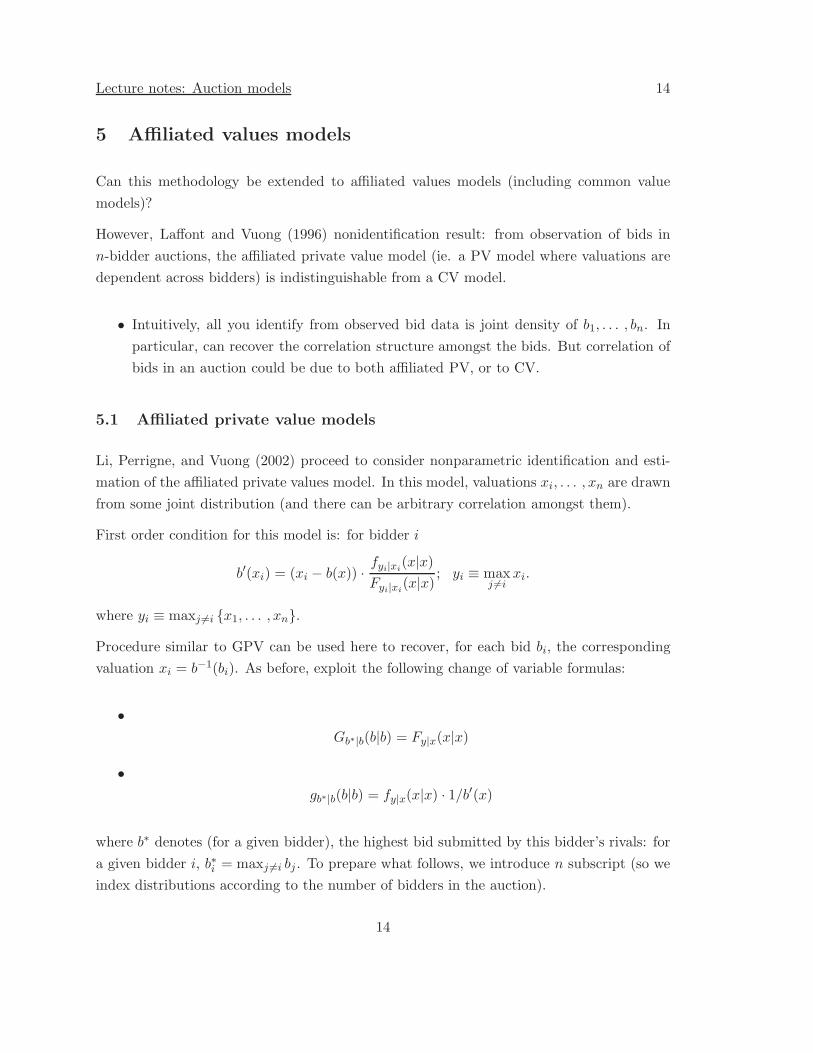
5 Affiliated values models
Can this methodology be extended to affiliated values models (including common value
models)?
However, Laffont and Vuong (1996) nonidentification result: from observation of bids in
n-bidder auctions, the affiliated private value model (ie. a PV model where valuations are
dependent across bidders) is indistinguishable from a CV model.
• Intuitively, all you identify from observed bid data is joint density of b1, . . . , bn. In
particular, can recover the correlation structure amongst the bids. But correlation of
bids in an auction could be due to both affiliated PV, or to CV.
5.1 Affiliated private value models
Li, Perrigne, and Vuong (2002) proceed to consider nonparametric identification and esti-
mation of the affiliated private values model. In this model, valuations xi, . . . , xn are drawn
from some joint distribution (and there can be arbitrary correlation amongst them).
First order condition for this model is: for bidder i
b′(xi) = (xi − b(x)) ·fyi|xi
(x|x)
Fyi|xi(x|x)
; yi ≡ maxj 6=i
xi.
where yi ≡ maxj 6=i {x1, . . . , xn}.
Procedure similar to GPV can be used here to recover, for each bid bi, the corresponding
valuation xi = b−1(bi). As before, exploit the following change of variable formulas:
•
Gb∗|b(b|b) = Fy|x(x|x)
•
gb∗|b(b|b) = fy|x(x|x) · 1/b′(x)
where b∗ denotes (for a given bidder), the highest bid submitted by this bidder’s rivals: for
a given bidder i, b∗i = maxj 6=i bj . To prepare what follows, we introduce n subscript (so we
index distributions according to the number of bidders in the auction).
14

Lecture notes: Auction models 15
Li, Perrigne, and Vuong (2000) suggest nonparametric estimates of the form
Gn(b; b) =1
Tn × h × n
T∑
t=1
n∑
i=1
K
(b − bit
h
)
1 (b∗it < b, nt = n)
gn(b; b) =1
Tn × h2 × n
T∑
t=1
n∑
i=1
1(nt = n)K
(b − bit
h
)
K
(b − b∗it
h
)
.
(10)
Here h and h are bandwidths and K(·) is a kernel. Gn(b; b) and gn(b; b) are nonparametric
estimates of
Gn(b; b) ≡ Gn(b|b)gn (b) =∂
∂bPr(B∗
it ≤ m,Bit ≤ b)|m=b
and
gn(b; b) ≡ gn(b|b)gn (b) =∂2
∂m∂bPr(B∗
it ≤ m,Bit ≤ b)|m=b
respectively, where gn(·) is the marginal density of bids in equilibrium. Because
Gn(b; b)
gn(b; b)=
Gn(b|b)
gn(b|b)(11)
Gn(b;b)gn(b;b) is a consistent estimator of Gn(b|b)
gn(b|b) . Hence, by evaluating Gn(·, ·) and gn(·, ·) at each
observed bid, we can construct a pseudo-sample of consistent estimates of the realizations
of each xit = b−1(bit) using Eq. (4):
xit =Gn(bit; bit)
gn(bit; bit). (12)
Subsequently, joint distribution of x1, . . . , xn can be recovered as sample joint distribution
of x1, . . . , xn.
5.2 Common value models: testing between CV and PV
Laffont-Vuong did not consider variation in n, the number of bidders.
In Haile, Hong, and Shum (2003), we explore how variation in n allows us to test for
existence of CV.
Introduce notation:
v(xi, xi, n) = E[Vi|Xi = xi,maxj 6=i
Xj = xi, n].
Recall the winner’s curse: it implies that v(x, x, n) is invariant to n for all x in a PV model
but strictly decreasing in n for all x in a CV model.
15
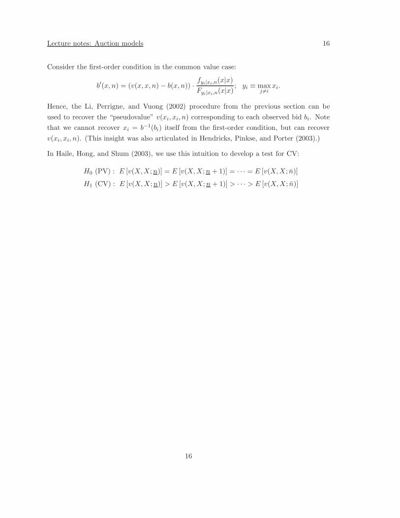
Lecture notes: Auction models 16
Consider the first-order condition in the common value case:
b′(x, n) = (v(x, x, n) − b(x, n)) ·fyi|xi,n(x|x)
Fyi|xi,n(x|x); yi ≡ max
j 6=ixi.
Hence, the Li, Perrigne, and Vuong (2002) procedure from the previous section can be
used to recover the “pseudovalue” v(xi, xi, n) corresponding to each observed bid bi. Note
that we cannot recover xi = b−1(bi) itself from the first-order condition, but can recover
v(xi, xi, n). (This insight was also articulated in Hendricks, Pinkse, and Porter (2003).)
In Haile, Hong, and Shum (2003), we use this intuition to develop a test for CV:
H0 (PV) : E [v(X,X;n)] = E [v(X,X;n + 1)] = · · · = E [v(X,X; n)]
H1 (CV) : E [v(X,X;n)] > E [v(X,X;n + 1)] > · · · > E [v(X,X; n)]
16

Lecture notes: Auction models 17
6 Revenue Equivalence, Optimal Auctions, and Linkage Prin-
ciple
6.1 Revenue Equivalence
Consider the auction as an example of a mechanism, which is a general scheme whereby
agents with private types v give a report v of their type (where possibly v 6= v). The auction
mechanism consists of two functions:
• T (v): payment agent must make if his report is v
• P (v): probability of winning the object if his report is v.
The surplus of an agent with type v, who reports that his type is v, is “quasilinear”:
S(v; v) ≡ vP (v) − T (v).
The seller’s mechanism design problem is to choose the functions P (·) and T (·) to maximize
his expected profits. By the “revelation principle” (for which the 2007 Nobel Laureate
Roger Myerson is most well known for), we can restrict attention to mechanisms which
satisfy an incentive compatibility condition, which requires that agents find it in their
best interest to report the truth.
The revenue equivalence result falls out as an implication of quasilinearity and incentive
compatibility. Assuming differentiability, incentive compatibility implies the following first-
order condition:
∂S(v; v)
∂v
∣∣∣∣v=v
= vP ′(v) − T ′(v) = 0. (13)
Hence, under an IC mechanism, the surplus of an agent with type v is just equal to
S(v) ≡ S(v; v) = vP (v) − T (v).
Given quasilinearity, instead of viewing the seller as setting P and T functions, can view
him as setting P and S functions, and T (v) = S(v) − vP (v).
By Eq. (13), we see that IC places restrictions on the S function that seller can choose.
Namely, the derivative of the S function must obey:
S′(v) = P (v) + vP ′(v) − T ′(v)
= P (v) + 0(14)
17

Lecture notes: Auction models 18
where the second line follows from Eq. (13). This operation is the “envelope condition”.
Hence, integrating up, the S function obeys
S(v) = S(v) +
∫ v
v
P (v)dv (15)
where v denotes the lowest type. From the above, we see that any IC-auction mechanism
with quasilinear preferences is completely characterized by (i) the quantity S(v), the surplus
gained by the lowest type; and (ii) P (·), the probability of winning.
Now note that, under independence of types, the monotonic equilibrium in the standard
auction forms (including first-price and second-price auctions) have the same P (v) function.
This is because the object is always awarded to the bidder with the highest type, so that
for any v, P (v) is just the probability that a bidder with type v has the highest type;
that is, with N bidders, and each type v distributed i.i.d. from distribution F (v), we have
P (v) = [F (v)]N−1. Furthermore, the standard auction forms also have the condition that
b(v) = v, so that S(v) = 0.
Hence, by quasilinearity, the standard auction forms also have the same T function, given
by T (v) = S(v) − vP (v). Since the T function is the revenue function for the seller, for
each type, we conclude that the standard auction forms give the seller the same expected
revenue.
6.2 Optimal auctions
Now consider the seller’s optimal choice of mechanism. As the discussion above showed,
we can just focus on the seller’s choice of S(v) and P (·). These are chosen to maximize
expected revenue from selling to each bidder, which is equal to
ER =
∫ v
v
T (v)f(v)dv
=
∫ v
v
[vP (v) − S(v)]f(v)dv
=
∫ v
v
vP (v)f(v)dv −
∫ v
v
f(v)[
∫ v
v
P (x)dx]dv −
∫ v
v
S(v)f(v)dv
=
∫ v
v
P (v)f(v)
[
v −1 − F (v)
f(v)
]
dv − S(v)
≡
∫ v
v
P (v)f(v)v∗dv.
(16)
18

Lecture notes: Auction models 19
The third equality follows by substituting in the IC constraint (15). The fourth equality
uses integration by parts to simplify the second term, with the substitution u =∫ v
vP (x)dx
and dv = f(v)dv. In the above, V ∗ is called the “virtual type” corresponding to a type v.
The interpretation is that the revenue that the seller makes from a bidder with type v is
v∗ ≤ v, so that the deviation 1−F (v)f(v) is the bidder’s “information rent” which arises because
only the bidder knows his type.
Under the additional assumption:
(∗)1 − F (v)
f(v)is decreasing in v
then v∗ is increasing in v.2 In this case, given a set of N bidders, the seller just wants
to award the object to the bidder with the highest report. To implement this, he will
set P (v) = Pr(v is highest out of N signals) = F (v)N−1. This is just like in the standard
auction forms.
However, because of the information rent, he will not be willing to sell to all bidders, but
only those with non-negative v∗. Thus he will set a reserve price, such that all bidders with
v∗ ≤ 0 are excluded. Let r∗ denote this optimal reserve price. Recall that, with a reserve
price r and IPV, the lower bound on bids is given by the condition b(r) = r, that is, the
reserve price r screens out bidders with valuations v ≤ r. Hence, the optimal reserve price
r∗ satisfies
r∗ −1 − F (r∗)
f(r∗)= 0.
r∗ depends on the distribution of types f(v). For example, if v ∼ U [0, 1], then
0 = r∗ −1 − F (r∗)
f(r∗)= r∗ −
1 − r∗
1= 2r∗ − 1 ⇒ r∗ =
1
2.
6.3 Linkage principle
See handout from Krishna (2002).
6.4 Important results under non-independence
The crucial assumption for the RET is independence of bidder types. This turns a compli-
cated multi-agent mechanism design problem to the single-agent problem, which was how
2In statistics, the quantity f(v)/[1 = F (v)] is called the hazard function, so that assumption (*) is
equivalently that the hazard function of v is increasing.
19
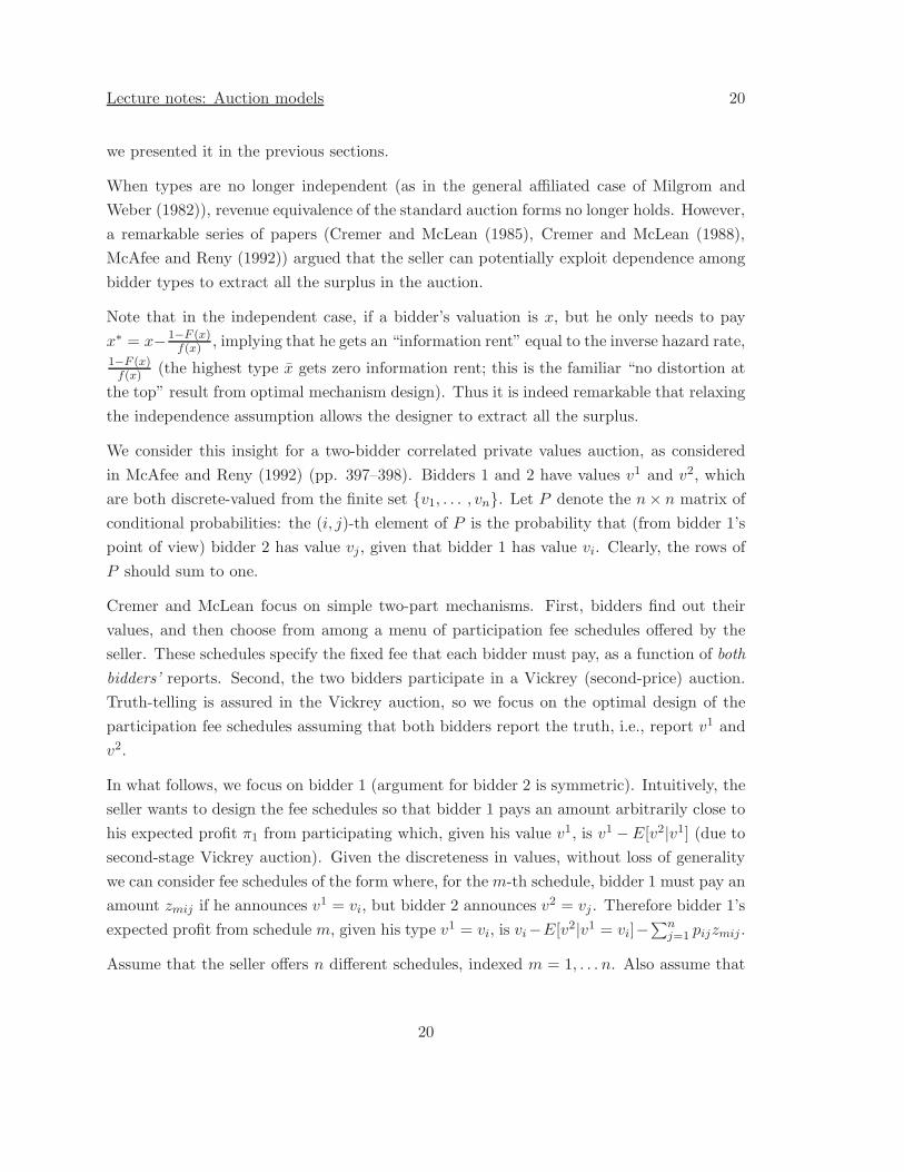
Lecture notes: Auction models 20
we presented it in the previous sections.
When types are no longer independent (as in the general affiliated case of Milgrom and
Weber (1982)), revenue equivalence of the standard auction forms no longer holds. However,
a remarkable series of papers (Cremer and McLean (1985), Cremer and McLean (1988),
McAfee and Reny (1992)) argued that the seller can potentially exploit dependence among
bidder types to extract all the surplus in the auction.
Note that in the independent case, if a bidder’s valuation is x, but he only needs to pay
x∗ = x− 1−F (x)f(x) , implying that he gets an “information rent” equal to the inverse hazard rate,
1−F (x)f(x) (the highest type x gets zero information rent; this is the familiar “no distortion at
the top” result from optimal mechanism design). Thus it is indeed remarkable that relaxing
the independence assumption allows the designer to extract all the surplus.
We consider this insight for a two-bidder correlated private values auction, as considered
in McAfee and Reny (1992) (pp. 397–398). Bidders 1 and 2 have values v1 and v2, which
are both discrete-valued from the finite set {v1, . . . , vn}. Let P denote the n× n matrix of
conditional probabilities: the (i, j)-th element of P is the probability that (from bidder 1’s
point of view) bidder 2 has value vj, given that bidder 1 has value vi. Clearly, the rows of
P should sum to one.
Cremer and McLean focus on simple two-part mechanisms. First, bidders find out their
values, and then choose from among a menu of participation fee schedules offered by the
seller. These schedules specify the fixed fee that each bidder must pay, as a function of both
bidders’ reports. Second, the two bidders participate in a Vickrey (second-price) auction.
Truth-telling is assured in the Vickrey auction, so we focus on the optimal design of the
participation fee schedules assuming that both bidders report the truth, i.e., report v1 and
v2.
In what follows, we focus on bidder 1 (argument for bidder 2 is symmetric). Intuitively, the
seller wants to design the fee schedules so that bidder 1 pays an amount arbitrarily close to
his expected profit π1 from participating which, given his value v1, is v1 −E[v2|v1] (due to
second-stage Vickrey auction). Given the discreteness in values, without loss of generality
we can consider fee schedules of the form where, for the m-th schedule, bidder 1 must pay an
amount zmij if he announces v1 = vi, but bidder 2 announces v2 = vj . Therefore bidder 1’s
expected profit from schedule m, given his type v1 = vi, is vi−E[v2|v1 = vi]−∑n
j=1 pijzmij .
Assume that the seller offers n different schedules, indexed m = 1, . . . n. Also assume that
20

Lecture notes: Auction models 21
zmij = vm − E[v2|v1 = vm] + αm ∗ xmj . Hence, the net expected payoff to bidder 1, who
has valuation vi, chooses schedule m, and then the bidders announce (vi, vj), are:
v1 − E[v2|v1 = vi] − (vm − E[v2|v1 = vm]) − αm
n∑
j=1
pijxmj .
It turns out that the parameter α will be the same across all schedules, and so we eliminate
the m subscript from these quantities.
In order for the seller to design schedules which extract all of bidder 1’s surplus, we require
that:
1. For each i = 1, . . . , n, there exists a vector ~xi ≡ (xi1, . . . , xin)′ such that
n∑
j=1
pijxij = 0,
n∑
j=1
pi′jxij ≤ 0, ∀i′ 6= i :
that is, the vector ~xi “separates” the i-th row of P from the other rows, at 0.
2. α must be set sufficiently large so that, for all i = 1, . . . , n, if bidder 1 has value v1 = vi
he will choose schedule i. This implies that his expected profit from choosing schedule
i exceeds that from choosing any schedule i′ 6= i. These incentive compatibility
conditions pin down α:
− α ∗
n∑
j=1
pijxij ≥ vi − E[v2|v1 = vi] − (vi′ − E[v2|v1 = vi′ ]) − α ∗
n∑
j=1
pijxi′j , ∀i′ 6= i
⇔0 ≥ vi − E[v2|v1 = vi] − (vi′ − E[v2|v1 = vi′ ]) − αi ∗n∑
j=1
pijxi′j, ∀i′ 6= i
⇔α > maxi′ 6=i
(vi − E[v2|v1 = vi]
)−(vi′ − E[v2|v1 = vi′ ]
)
∑nj=1 pijxi′j
.
A sufficient condition for the first point above is that, for all i = 1, . . . , n, the i-th row
of P is not in the (n-dimensional) convex set spanned by all the other rows of P .3 Then
we can apply the separating hyperplane theorem to say that there always exists a vector
(xi1, . . . , xin)′ which separates the i-th row of P from the convex set composed of convex
combinations of the other n − 1 rows of P .
3Or, using terminology in McAfee and Reny (1992), the i-th row of P is not in the convex hull of the
other n − 1 rows of P .
21

Lecture notes: Auction models 22
In order for the i-th row of P is not in the (n-dimensional) convex set spanned by all the
other rows of P , we require that the i-th row of P cannot be written as a linear combination
of the other n − 1 rows, i.e., that all the rows of P are linear independent. As Cremer and
McLean (1988) note, this is a full rank condition on P .
As an example, consider the case where the P matrix is diagonal (that is, pii = 1 for all
i = 1, . . . , n). This is the case of “Stalin’s food taster”. In this case, the vector ~xi with
element xii = 0 and xij = −1 for j 6= i satisfies point 1. The numerator of the expression
for α is equal to 0. Thus any arbitrarily small participation fee will lead to full surplus
extraction!
References
Akerlof, G. (1970): “The Market for ”Lemons”: Quality Uncertainty and the Market Mechanism,”
Quarterly Journal of Economics, 84, 488–500.
Athey, S., and P. Haile (2002): “Identification of Standard Auction Models,” Econometrica, 70,
2107–2140.
Cremer, J., and R. McLean (1985): “Optimal Selling Strategies under Uncertainty for a Dis-
criminating Monopolist when Demands are Interdependent Strategy Auctions,” Econometrica,
53, 345–361.
(1988): “Full Extraction of the Surplus in Bayesian and Dominant Strategy Auctions,”
Econometrica, 56, 1247–1257.
Glosten, L., and P. Milgrom (1985): “Bid, ask, and transactions prices in a specialist market
with heterogeneiously informed traders,” Journal of Financial Economics, 14.
Guerre, E., I. Perrigne, and Q. Vuong (2000): “Optimal Nonparametric Estimation of First-
Price Auctions,” Econometrica, 68, 525–74.
Haile, P., H. Hong, and M. Shum (2003): “Nonparametric Tests for Common Values in First-
Price Auctions,” NBER working paper #10105.
Hendricks, K., J. Pinkse, and R. Porter (2003): “Empirical Implications of Equilibrium
Bidding in First-Price, Symmetric, Common-Value Auctions,” Review of Economic Studies, 70,
115–145.
Klemperer, P. (1999): “Auction Theory: A Guide to the Literature,” Journal of Economic Sur-
veys, 13, 227–286.
Krishna, V. (2002): Auction Theory. Academic Press.
22

Lecture notes: Auction models 23
Laffont, J. J., H. Ossard, and Q. Vuong (1995): “Econometrics of First-Price Auctions,”
Econometrica, 63, 953–980.
Laffont, J. J., and Q. Vuong (1996): “Structural Analysis of Auction Data,” American Eco-
nomic Review, Papers and Proceedings, 86, 414–420.
Lewis, G. (2007): “Asymmetric Information, Adverse Selection and Seller Revelation on eBay
Motors,” Harvard University, mimeo.
Li, T., I. Perrigne, and Q. Vuong (2000): “Conditionally Independent Private Information in
OCS Wildcat Auctions,” Journal of Econometrics, 98, 129–161.
(2002): “Structural Estimation of the Affiliated Private Value Acution Model,” RAND
Journal of Economics, 33, 171–193.
McAfee, P., and P. Reny (1992): “Correlated Information and Mechanism Design,” Economet-
rica, 60, 395–421.
Milgrom, P., and N. Stokey (1982): “Information, Trade and Common Knowledge,” Journal
of Economic Theory, 26, 17–27.
Milgrom, P., and R. Weber (1982): “A Theory of Auctions and Competitive Bidding,” Econo-
metrica, 50, 1089–1122.
Myerson, R. (1981): “Optimal Auction Design,” Mathematics of Operation Research, 6, 58–73.
23


![Home [] · From May to June 2019, the MDB held further education and awareness ... EC102 EC104 EC105 EC106 EC108 EC109 EC121 EC122 EC123 EC124 EC126 Categöry Category A (Metro) Category](https://static.fdocuments.us/doc/165x107/5f7698f0fa2929366d3fbe14/home-from-may-to-june-2019-the-mdb-held-further-education-and-awareness-.jpg)