1

The Solar MURI Effort: Recent Results, Directions for the Future

George Fisher

SSL, UC Berkeley

2

Overall vision of our MURI effort

• Develop a time dependent, physics-based forward model of the Sun and heliosphere that takes as input time sequences of real vector magnetic field observations from the solar atmosphere.

Required components:

• Understanding CME eruption mechanisms• State-of-the-art solar magnetic data and

analysis techniques• A formalism that can incorporate magnetic

data into MHD models• MHD techniques that can cope with greatly

varying temporal and spatial scales

3

The Solar MURI project involves team members from 9 Universities:

• UC Berkeley• University of Colorado• Stanford University• Drexel University• University of New

Hampshire• Montana State University• UC San Diego • Big Bear Solar Observatory

(NJIT)• University of Hawaii

4

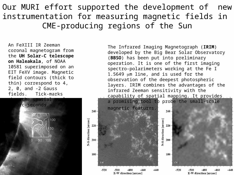
Our MURI effort supported the development of new instrumentation for measuring magnetic fields in

CME-producing regions of the Sun

An FeXIII IR Zeeman coronal magnetogram from the UH Solar-C telescope on Haleakala, of NOAA 10581 superimposed on an EIT FeXV image. Magnetic field contours (thick to thin) correspond to 4, 2, 0, and -2 Gauss fields. Tick-marks show the spatial scale in arc-seconds.

The Infrared Imaging Magnetograph (IRIM) developed by the Big Bear Solar Observatory (BBSO) has been put into preliminary operation. It is one of the first imaging spectro-polarimeters working at the Fe I 1.5649 m line, and is used for the observation of the deepest photospheric layers. IRIM combines the advantages of the infrared Zeeman sensitivity with the capability of spatial mapping. It provides a promising tool to probe the small-scale

magnetic features.

5

CME initiation physics

Research by team member Terry Forbes (UNH) studying the physics of line-tied twisted flux ropes, was able to show that such initial configurations can explain (1) eruption without escape, (2) out-of-plane twisting motion, and (3) formation of aneurism-like structures

Alfven Mach No.

Density

‘Breakout’ model eruptions carried out by Gimin Gao and Peter MacNeice (Drexel University) of asymmetric configurations – high resolution study of shock structures with potential for particle acceleration.

6

Numerical Simulation of Interplanetary CME Propagation

Remote observations of the photospheric magnetic field

Remote observations of the coronal mass ejection (CME)

Plasma cloud is ejected into interplanetary space

Interplanetary shock and ejecta are approaching Earth

APPROACH

• Use available remote observations of solar activity for WSA (Arge et al.) and cone (Zhao et al.) models (Stanford)

• Use outputs from the above models for 3-D magneto-hydrodynamic model (U. Colorado - Odstrcil et al.)

FOLLOW-ON USE OF BASIC RESEARCH RESULTS FROM MURI

• NSF/Center for Integrated Space Weather Modeling (CISM) has incorporated the system for development of their solar-energetic-particle models

• NOAA/Space Environment Center is incorporating the system for prediction of solar wind parameters at EarthPI: Dusan Odstrcil, University of Colorado & NOAA/SEC

contours = density in equatorial planecolor = velocity at boundary and ejecta

7

Observe how CMEs propagate to through the interplanetary medium to 1AU

SMEI observations of the January 20, 2005 CME, shown in a remote-view presentation for the same time. The view is from 30˚ above the ecliptic plane and about 30˚ west of the Sun-Earth line. There is little or no evidence that the bulk of the CME mass reached Earth (shown as a blue dot) even though the solar energetic particles associated with the event arrived within 20 minutes of the event onset, and the shock associated with the CME event reached the Earth on about 18 UT January 21.

8

Conclusions about the most critical research that will follow from this project:

• We must resolve the basic physics of the “CME Initiation” problem before comprehensive Sun-heliosphere system models will have any real predictive capability. This will be accomplished with the analysis of better data of the pre-CME coronal and chromospheric evolution to be taken with upcoming NASA missions (Solar-B, Stereo, and SDO), new high-resolution ground-based data, and by careful comparisons of this data with existing and future theoretical models. This focus-topic was one of those recommended by the steering committee for LWS-TR&T, because of its importance for the future of space weather models.

• We must continue the development of techniques that allow the incorporation of vector magnetic field data into time dependent models of flare and CME producing regions of the Sun. This capability is required by any realistic Sun-heliosphere model with predictive capability.

• The remainder of this talk is an outline for carrying out this research by members of our group at UC Berkeley and collaborators.

9

Developing the techniques for determining the dynamics of magnetic fields at the photosphere,

needed for dynamic models of the corona:Data Driving --- The Strategy:

Observational Data / MEF, ILCT

“Active” Boundary Layer

Model Corona

10

The objective:

• To directly incorporate observations of the vector magnetic field at the photosphere (or chromosphere) into physics-based dynamic models of the solar atmosphere

The requirements:

(1) Sequences of reduced, ambiguity-resolved vector magnetograms of sufficient quality to incorporate into an MHD code

(2) A robust method of determining the electric field consistent with boththe observed evolution of the photospheric field and Faraday’s Law

(3) An MHD code (or set of coupled codes) capable of modeling a regionencompassing the photosphere (where relatively reliable measurements of the magnetic field are available), chromosphere, transition region andcorona

(4) A physically self-consistent means of incorporating (1) and (2) into (3)

11

(1) Understand sequences of reduced, high-quality, ambiguity-resolved vector magnetograms well enough to incorporate them into a numerical simulation

• What magnetic field data provide the most important information about the state of the solar atmosphere, and how do we prepare the data and make best use of it?

• What is the best way to generate the initial atmosphere of a time-dependent calculation; one that is both physically meaningful, and consistent with the relevant observations of the corona? (current method: the “optimization technique”, e.g., Wheatland et al. 2000)

• How do we best describe the evolution of a model photosphere given the evolution of, and noise in, the observed data and our best understanding of the most important physics?

We currently rely on our colleagues from our SHINE-funded collaboration with CoRA and MSU to obtain quality measurements of active region vector magnetic fields, and to address each of these questions prior to attempting to incorporate a given dataset into a numerical calculation. (e.g., IVM data: AR8210, May 1998; AR9046, June 2000; AR10030, July 2002; AR10725, Feb 2005)

12

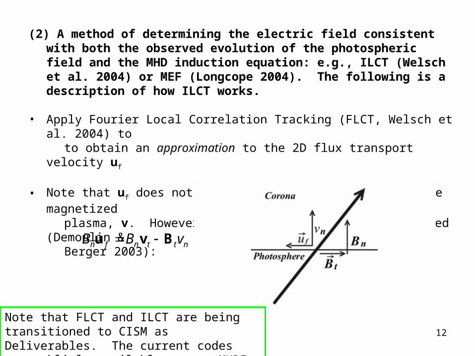
(2) A method of determining the electric field consistent with both the observed evolution of the photospheric field and the MHD induction equation: e.g., ILCT (Welsch et al. 2004) or MEF (Longcope 2004). The following is a description of how ILCT works.

• Apply Fourier Local Correlation Tracking (FLCT, Welsch et al. 2004) to to obtain an approximation to the 2D flux transport velocity uf

• Note that uf does not represent the 3D flow field of the magnetized plasma, v. However, the two are geometrically related (Demoulin & Berger 2003):

nttnfn vBB Bvu

Note that FLCT and ILCT are being transitioned to CISM as Deliverables. The current codes are publicly available on our MURI website.

13

0

tntntn vBt

BBv

0

fnnn Bt

Bu

To demonstrate how ILCT relates the MHD induction equation to the fluxtransport velocity, consider the vertical component of the ideal MHD induction equation (here, for clarity, we neglect the resistive term --- in general, it can be included):

nu ttfnB

Substituting the geometric relation of the previous slide, we have:

Now, simply define Bnuf in the following way:

Substituting this expression into (1) yields

(1)

2tn

t

B

Since the LHS is known, we

have a Poisson equation for φthat can be easily solved.

(2)

14

Note that to obtain v, we must appeal to the fact that field-aligned flowsare unconstrained by the induction equation (one way of closing the systemis to simply assume ).

Taking the curl of (2), we have

If we assume that u(FLCT) (our LCT approximation of uf) represents a trueflux transport velocity, we again have a solvable Poisson equation. Withboth scalar potentials known, we can determine a flux transport velocity thatis both consistent with the observed evolution of the photospheric field and the MHD induction equation:

Up to this point, the analysis only requires the normal component ofthe magnetic field! The vector field is necessary only when extractingthe 3D flow field from

2tfnt B nu

nu ttfnB

n

nttf B

vBvu

0Bv

15

Brian Welsch has recently implemented a preliminary, automated“Magnetic Evolution Pipeline” (MEP):

• New MDI magnetograms are automatically downloaded (cron checks for new magnetograms using wget), de-projected, and tracked using FLCT

• The output stream includes de-projected magnetograms, FLCT flows (.png graphics files and ASCII data files), and tracking parameters

• Full documentation and all codes (including possible bugs!) are currently online

http://solarmuri.ssl.berkeley.edu/~welsch/public/data/Pipeline/

16

Validation of ILCT, MEF and other similar methods: Use artificial magnetograms from MHD

simulations where the solutions are known

(Note that the MHD code used for this purpose, ANMHD, is publicly available from our MURI website, and is slated to be assimilated by CCMC)

17

Validation of velocity inversion techniques:

FLCT

MEF

ILCT

zE)(

18

Validation of velocity inversion techniques: vx, vy, vz

FLCT

MEF

ILCT

19

(3) An MHD code (or set of coupled codes) capable of modeling a region encompassing the photosphere, chromosphere, transition region and corona

Some realities:

Extreme spatial and temporal disparities• small-scale, active region, and global features are fundamentally inter-

connected • magnetic features at the photosphere are long-lived (relative to the

convective turnover time) while features in the magnetized corona can evolve rapidly (e.g., topological changes following reconnection events)

Vastly different physical regimes• photosphere and below: relatively dense, turbulent (high-β) plasma with

strong magnetic fields organized in isolated structures • corona: field-filled, low-density, magnetically dominated plasma (at least

around strong concentrations of magnetic flux!)• flow speeds in CZ below the surface are typically below the characteristic

sound and Alfven speeds, while the chromosphere, transition region and corona are often shock-dominated

20

…different physical regimes (cont’d)

• corona: energetics dominated by optically thin radiative cooling, anisotropic thermal conduction, and some form of coronal heating consistent with the empirical relationship of Pevtsov et al. 2003 (energy dissipation as measured by soft X-rays proportional to the measured unsigned magnetic flux at the photosphere)

• photosphere/chromosphere: energetics dominated by optically thick radiative transitions

Additional computational challenges:

A dynamic model atmosphere extending from at or below the photosphere to the corona must:

• span a ~10 order of magnitude change in gas density and a thermodynamic transition from the 1MK corona to the optically thick, cooler layers of the low atmosphere, visible surface, and below

• resolve a ~100km photospheric pressure scale height (energy scale height in the transition region can be as small as 1km!) while following large-scale evolution

21

Toward more realistic AR models:

We must solve the following system:

Energy source terms (Q) include:

• Optically thin radiative cooling

• Anisotropic thermal conduction

• An option for an empirically-based coronal heating mechanism --- must maintain a corona consistent with the empirical constraint of Pevtsov (2003)

• LTE optically thick cooling (options: solve the grey transfer equation in the 3D Eddington approximation, or use a simple parameterization that maintains the super-adiabatic gradient necessary to initiate and maintain convective turbulence)

22

Surmounting practical computational challenges

• The MHD system is solved semi-implicitly on a block adaptive mesh.

• The non-linear portion of the system is treated explicitly using the semi-discrete central method of Kurganov-Levy (2000) using a 3rd-order CWENO polynomial reconstruction

– Provides an efficient shock capture scheme, AMR is not required to resolve shocks

• The implicit portion of the system, the contributions of the energy source terms, and the resistive and viscous contributions to the induction and momentum equations respectively, is solved via a “Jacobian-free” Newton-Krylov technique

– Makes it possible to treat the system implicitly (thereby providing a means to deal with temporal disparities) without prohibitive memory constraints

23

Quiet Sun relaxation run (serial test):

12

24

Toward AR scale: MPI-AMR relaxation run (test)

The near-term plan:

• Dynamically and energetically relax a 30Mm square Cartesian domain extending to ~2.5Mm below the surface.

• Introduce a highly-twisted AR-scale magnetic flux rope (from the top of a sub-surface calculation) through the bottom boundary of the domain

• Reproduce (hopefully!) a highly sheared, δ-spot type AR at the surface, and follow the evolution of the model corona as AR flux emerges into, reconnects and reconfigures coronal fields

The long term plan:

• global scales / spherical geometry

25

(4) Towards a physically self-consistent means of incorporating (1) and (2) into (3): The “Active Boundary Layer”

Use AMPS as essentially two, fully coupled codes: a thin, dynamic photospheric layer actively coupled (internally; i.e., not via a framework) to the AMPS domain

• Within the thin, photospheric boundary layer, the continuity, induction, and energy equations are solved given an ILCT flow field (assumed to permeate the entirety of the thin layer). • This active boundary is dynamically coupled to AMPS, which solves the full MHD system in a domain that extends from the top of the model photosphere into the transition region and low corona

Inherent physical assumption: Coronal forces do not affect the photosphere

This internally-coupled system could instead extend to the lowtransition region, and then be externally coupled to existing Coronal models whose lower boundaries necessarily reside in the transition region.

26

Observational Data / ILCT

“Active” Boundary Layer

Model Corona

Summary Picture of the Overall System

27

Summary (where we’re at):

(1) Sequences of reduced, ambiguity-resolved vector magnetograms of sufficient quality to incorporate into an MHD code

--- we look forward to the increasing availability of sequences of quality vector magnetograms

(2) A robust method of determining the electric field consistent with both the observed evolution of the photospheric magnetic field and Faraday’s Law

--- complete

(3) An MHD code (or set of coupled codes) capable of modeling a region encompassing the photosphere (where relatively reliable measurements of the magnetic field are available), chromosphere, transition region and low corona

--- almost there….

(4) A physically self-consistent means of incorporating (1) and (2) into (3)

--- still working on it! Hope to have something to present at SHINE…