1 © The McGraw-Hill Companies, Inc., 2004 Chapter 12 Forecasting and Demand Management.

1

©The McGraw-Hill Companies, Inc., 2004

Chapter 12

Forecasting and Demand

Management

2


• Educated Guessing Game

• Demand Management

• Qualitative Forecasting Methods

• Simple & Weighted Moving Average Forecasts

• Exponential Smoothing

• Simple Linear Regression

• Web-Based Forecasting

OBJECTIVES

3


• Guessing at the future

• Seldom correct

— No perfect forecast

— Objective is to minimize forecast errors

• It is only a tool used to set:

— Production plan and budgets

— Work schedules

Characteristics of Forecasts

4


• Forecasts are more accurate in aggregation

• Long-term forecasts are less accurate than short-term forecasts

• Forecasts are means to an end

Characteristics of Forecasts

5


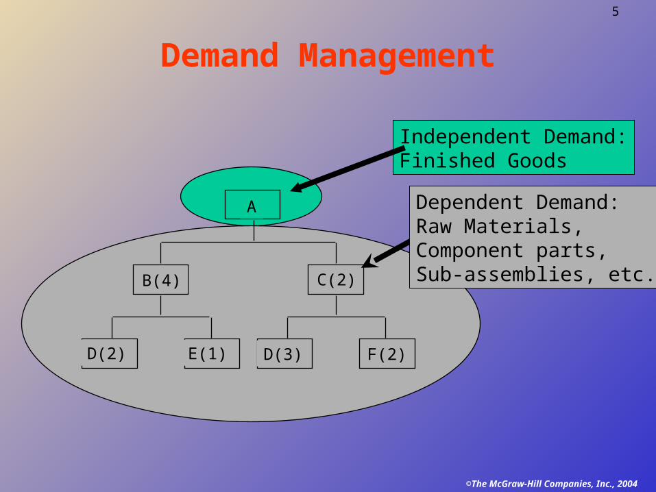
Demand Management

A

B(4) C(2)

D(2) E(1) D(3) F(2)

Dependent Demand:Raw Materials, Component parts,Sub-assemblies, etc.

Independent Demand:Finished Goods

6


Independent Demand: What a firm can do to manage it?

• Can take an active role to influence demand— Offer incentive to customers— Wage campaigns to sell products

• Can take a passive role and simply respond to demand — Especially if at full capacity— High cost of advertisement

7


Types of Forecasts

• Qualitative (Judgmental)— Forecasts based on subjective estimates and

opinions

• Quantitative— Time Series Analysis— Causal Relationships

— Simulation

8


Components of Demand

• Average demand for a period of time

• Trend• Seasonal element• Cyclical elements• Random variation• Autocorrelation

9


Finding Components of Demand

1 2 3 4

x

x xx

xx

x xx

xx x x x

xxxxxx x x

xx

x x xx

xx

xx

x

xx

xx

xx

xx

xx

xx

x

x

Year

Sal

es

Seasonal variationSeasonal variation

Linear

Trend

Linear

Trend

10


Qualitative Methods

Grass Roots

Market Research

Panel Consensus

Executive Judgment

Historical analogy

Delphi Method

Qualitative

Methods

11


Qualitative Methods

• Grass roots— Builds forecast by adding successively from

bottom— Those closest to customer know better

• Market research — Consumer surveys and interviews— Used to improve existing products

• Panel consensus — Open meetings with free exchange of ideas— Power play possibilities

12


Qualitative Methods

• Executive Judgment— Used for new products introduction— Decisions are broader and at a higher level

• Historical Analogy — Existing product used as a model for another— Example: buying CDs on Internet put you in

mailing list for related products

• Delphi Method

13


Delphi Method

l. Choose the experts to participate representing a variety of knowledgeable people in different areas

2. Through a questionnaire (or E-mail), obtain forecasts (and any premises or qualifications for the forecasts) from all participants

3. Summarize the results and redistribute them to the participants along with appropriate new questions

4. Summarize again, refining forecasts and conditions, and again develop new questions

5. Repeat Step 4 as necessary and distribute the final results to all participants

14


Time Series Analysis

• Time series forecasting models try to predict the future based on past data

• You can pick models based on:

1. Time horizon to forecast

2. Data availability

3. Accuracy required

4. Size of forecasting budget

5. Availability of qualified personnel

15


Simple Moving Average

• Assumes steady market demand

• Average of known demand series, n (order)

• Longer periods tend to be more reliable

• Longer periods tend to be less sensitive to demand shifts

• Maintains large database

• Equal weights given to all data

• Masks effect demand signals

16


Simple Moving Average Formula

F = A + A + A +...+A

ntt-1 t-2 t-3 t-nF =

A + A + A +...+A

ntt-1 t-2 t-3 t-n

• The simple moving average model assumes an average is a good estimator of future behavior

• The formula for the simple moving average is:

Ft = Forecast for the coming period n = Number of periods to be averagedA t-1 = Actual occurrence in the past

period for up to “n” periods

17


Simple Moving Average Problem (1)

Week Demand1 6502 6783 7204 7855 8596 9207 8508 7589 892

10 92011 78912 844

F = A + A + A +...+A

ntt-1 t-2 t-3 t-nF =

A + A + A +...+A

ntt-1 t-2 t-3 t-n

Question: What are the 3-week and 6-week moving average forecasts for demand? Assume you only have 3 weeks and 6 weeks of actual demand data for the respective forecasts

Question: What are the 3-week and 6-week moving average forecasts for demand? Assume you only have 3 weeks and 6 weeks of actual demand data for the respective forecasts

Week Demand 3-Week 6-Week1 6502 6783 7204 785 682.675 859 727.676 920 788.007 850 854.67 768.678 758 876.33 802.009 892 842.67 815.33

10 920 833.33 844.0011 789 856.67 866.5012 844 867.00 854.83

F4=(650+678+720)/3

=682.67F7=(650+678+720 +785+859+920)/6

=768.67

Calculating the moving averages gives us:


18

19


500

600

700

800

900

1000

1 2 3 4 5 6 7 8 9 10 11 12

Week

Dem

and

Demand

3-Week

6-Week

Plotting the moving averages and comparing them shows how the lines smooth out to reveal the overall upward trend in this example

Plotting the moving averages and comparing them shows how the lines smooth out to reveal the overall upward trend in this example

Note how the 3-Week is smoother than the Demand, and 6-Week is even smoother

Note how the 3-Week is smoother than the Demand, and 6-Week is even smoother

20


Simple Moving Average Problem (2) Data

Week Demand1 8202 7753 6804 6555 6206 6007 575

Question: What is the 3 week moving average forecast for this data?

Assume you only have 3 weeks and 5 weeks of actual demand data for the respective forecasts

Question: What is the 3 week moving average forecast for this data?

Assume you only have 3 weeks and 5 weeks of actual demand data for the respective forecasts

21


Simple Moving Average Problem (2) Solution

Week Demand 3-Week 5-Week1 8202 7753 6804 655 758.335 620 703.336 600 651.67 710.007 575 625.00 666.00

F4=(820+775+680)/3

=758.33F6=(820+775+680 +655+620)/5 =710.00

22


Weighted Moving Average

• More flexible than simple moving average

• Weights each data differently to vary their effect on the forecast

• Sum of weights must be = 1 if fractions

• Otherwise, weights can be real numbers. If so divide by sum of weights:

• Removes masking effect of moving average

- Ft = iti wDw /1

23


Weighted Moving Average Formula

F = w A + w A + w A +...+w At 1 t-1 2 t-2 3 t-3 n t-nF = w A + w A + w A +...+w At 1 t-1 2 t-2 3 t-3 n t-n

w = 1ii=1

n

w = 1ii=1

n

While the moving average formula implies an equal weight being placed on each value that is being averaged, the weighted moving average permits an unequal weighting on prior time periods

While the moving average formula implies an equal weight being placed on each value that is being averaged, the weighted moving average permits an unequal weighting on prior time periods

wt = weight given to time period “t” occurrence (weights must add to one)

wt = weight given to time period “t” occurrence (weights must add to one)

The formula for the moving average is:The formula for the moving average is:

24


Weighted Moving Average Problem (1) Data

Weights: t-1 .5t-2 .3t-3 .2

Week Demand1 6502 6783 7204

Question: Given the weekly demand and weights, what is the forecast for the 4th period or Week 4?

Question: Given the weekly demand and weights, what is the forecast for the 4th period or Week 4?

Note that the weights place more emphasis on the most recent data, that is time period “t-1”

Note that the weights place more emphasis on the most recent data, that is time period “t-1”

25


Weighted Moving Average Problem (1) Solution

Week Demand Forecast1 6502 6783 7204 693.4

F4 = 0.5(720)+0.3(678)+0.2(650)=693.4

26


Weighted Moving Average Problem (2)

Data

Weights: t-1 .7t-2 .2t-3 .1

Week Demand1 8202 7753 6804 655

Question: Given the weekly demand information and weights, what is the weighted moving average forecast of the 5th period or week?

Question: Given the weekly demand information and weights, what is the weighted moving average forecast of the 5th period or week?

27


Weighted Moving Average Problem (2) Solution

Week Demand Forecast1 8202 7753 6804 6555 672

F5 = (0.1)(755)+(0.2)(680)+(0.7)(655)= 672

28


Exponential Smoothing

• This is a form of moving average

• Relatively easy to use

• Requires minimal amount of data storage— Most recent forecast— Most recent demand— A smoothing constant

• One of most widely used forecasting method

• They are relatively accurate

29


Exponential Smoothing Model

• Premise: The most recent observations might have the highest predictive value

• Therefore, we should give more weight to the more recent time periods when forecasting

Ft = Ft-1 + a(At-1 - Ft-1)Ft = Ft-1 + a(At-1 - Ft-1)

constant smoothing Alpha

period epast t tim in the occurance ActualA

period past time 1in alueForecast vF

period t timecoming for the lueForcast vaF

:Where

1-t

1-t

t

30


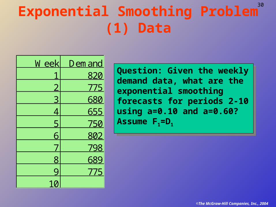
Exponential Smoothing Problem (1) Data

Week Demand1 8202 7753 6804 6555 7506 8027 7988 6899 775

10

Question: Given the weekly demand data, what are the exponential smoothing forecasts for periods 2-10 using a=0.10 and a=0.60?Assume F1=D1

Question: Given the weekly demand data, what are the exponential smoothing forecasts for periods 2-10 using a=0.10 and a=0.60?Assume F1=D1

31


Week Demand 0.1 0.61 820 820.00 820.002 775 820.00 820.003 680 815.50 793.004 655 801.95 725.205 750 787.26 683.086 802 783.53 723.237 798 785.38 770.498 689 786.64 787.009 775 776.88 728.20

10 776.69 756.28

Answer: The respective alphas columns denote the forecast values. Note that you can only forecast one time period into the future.

Answer: The respective alphas columns denote the forecast values. Note that you can only forecast one time period into the future.

32


Exponential Smoothing Problem (1) Plotting

500

600

700

800

900

1 2 3 4 5 6 7 8 9 10

Week

Dem

and

Demand

0.1

0.6

Note how that the smaller alpha results in a smoother line in this example

Note how that the smaller alpha results in a smoother line in this example

33


Exponential Smoothing Problem (2) Data

Question: What are the exponential smoothing forecasts for periods 2-5 using a =0.5?

Assume F1=D1

Question: What are the exponential smoothing forecasts for periods 2-5 using a =0.5?

Assume F1=D1

Week Demand1 8202 7753 6804 6555

34


Exponential Smoothing Problem (2) Solution

Week Demand 0.51 820 820.002 775 820.003 680 797.504 655 738.755 696.88

F1=820+(0.5)(820-820)=820 F3=820+(0.5)(775-820)=797.75

35


Simple Linear Regression Model

0 1 2 3 4 5 x (Time)

YThe simple linear regression model seeks to fit a line through various data over time

The simple linear regression model seeks to fit a line through various data over time

Is the linear regression modelIs the linear regression model

a

Yt = a + bxYt is the regressed forecast value or dependent variable in the model,a is the y-intercept value of the the regression line, andb is similar to the slope of the regression line. However, since it is calculated with the variability of the data in mind, its formulation is not as straight forward as our usual notion of slope.

36


Simple Linear Regression Formulas for Calculating “a” and “b”

a = y - bx

b =xy - n(y)(x)

x - n(x2 2

)

a = y - bx

b =xy - n(y)(x)

x - n(x2 2

)

37


Simple Linear Regression Problem Data

Week Sales1 1502 1573 1624 1665 177

Question: Given the data below, what is the simple linear regression model that can be used to predict sales in future weeks?

Question: Given the data below, what is the simple linear regression model that can be used to predict sales in future weeks?

Week Week*Week Sales Week*Sales1 1 150 1502 4 157 3143 9 162 4864 16 166 6645 25 177 8853 55 162.4 2499

Average Sum Average Sum

b =xy - n(y)(x)

x - n(x=

2499 - 5(162.4)(3)=

a = y - bx = 162.4 - (6.3)(3) =

2 2

) ( )55 5 9

63

106.3

143.5

b =xy - n(y)(x)

x - n(x=

2499 - 5(162.4)(3)=

a = y - bx = 162.4 - (6.3)(3) =

2 2

) ( )55 5 9

63

106.3

143.5

Answer: First, using the linear regression formulas, we can compute “a” and “b”

Answer: First, using the linear regression formulas, we can compute “a” and “b”

38

Yt = 143.5 + 6.3x

180

Period

135140145150155

160165170175

1 2 3 4 5

Sal

es

Sales

Forecast

The resulting regression model is:

Now if we plot the regression generated forecasts against the actual sales we obtain the following chart:

39

40


Forecast Errors

• Sources of errors

— Projecting the past into the future

— Wrong relationships

— Wrong information (data)

— Errors outside of our control

• Goal is to minimize the errors

41


The MAD Statistic to Determine Forecasting Error

MAD = A - F

n

t tt=1

n

MAD =

A - F

n

t tt=1

n

1 MAD 0.8 standard deviation

1 standard deviation 1.25 MAD

• The ideal MAD is zero which would mean there is no forecasting error

• The larger the MAD, the less accurate the resulting model

42


MAD Problem Data

Month Sales Forecast1 220 n/a2 250 2553 210 2054 300 3205 325 315

Question: What is the MAD value given the forecast values in the table below?

Question: What is the MAD value given the forecast values in the table below?

43


MAD Problem Solution

MAD = A - F

n=

40

4= 10

t tt=1

n

MAD =

A - F

n=

40

4= 10

t tt=1

n

Month Sales Forecast Abs Error

1 220 n/a

2 250 255 5

3 210 205 5

4 300 320 20

5 325 315 10

40

Note that by itself, the MAD only lets us know the mean error in a set of forecasts

Note that by itself, the MAD only lets us know the mean error in a set of forecasts

44


Tracking Signal Formula

• The Tracking Signal or TS is a measure that indicates whether the forecast average is keeping pace with any genuine upward or downward changes in demand.

• Depending on the number of MAD’s selected, the TS can be used like a quality control chart indicating when the model is generating too much error in its forecasts.

• The TS formula is:

TS =RSFE

MAD=

Running sum of forecast errors

Mean absolute deviationTS =

RSFE

MAD=

Running sum of forecast errors

Mean absolute deviation

45


Web-Based Forecasting: CPFR Defined

• Collaborative Planning, Forecasting, and Replenishment (CPFR) a Web-based tool used to coordinate demand forecasting, production and purchase planning, and inventory replenishment between supply chain trading partners.

• Used to integrate the multi-tier or n-Tier supply chain, including manufacturers, distributors and retailers.

• CPFR’s objective is to exchange selected internal information to provide for a reliable, longer term future views of demand in the supply chain.

• CPFR uses a cyclic and iterative approach to derive consensus forecasts.

46


Web-Based Forecasting: Steps in CPFR

• 1. Creation of a front-end partnership

agreement

• 2. Joint business planning

• 3. Development of demand forecasts

• 4. Sharing forecasts

• 5. Inventory replenishment

1 © The McGraw-Hill Companies, Inc., 2004 Chapter 12 Forecasting and Demand Management.

Documents

Transcript of 1 © The McGraw-Hill Companies, Inc., 2004 Chapter 12 Forecasting and Demand Management.