1

The Impacts of Dust on Regional Tropospheric Chemistry During the ACE-ASIA 1 Experiment: A Model Study with Observations 2

3 Youhua Tang1, Gregory R. Carmichael1, Gakuji Kurata2, Itsushi Uno3, Rodney J. Weber4, Chul-4

Han Song4, Sarath K. Guttikunda1, Jung-Hun Woo1, David G. Streets5, Cao Wei1, Antony D. 5

Clarke6, Barry Huebert6, and Theodore L. Anderson7 6 7 1 Center for Global and Regional Environmental Research, University of Iowa, Iowa, USA 8 2 Department of Ecological Engineering, Toyohashi University of Technology, Toyohashi, Japan 9 3 Research Institute for Applied Mechanics, Kyushu University, Fukuoka, Japan 10 4 School of Earth and Atmospheric Sciences, Georgia Institute of Technology, Georgia, USA 11 5 Decision and Information Sciences Division, Argonne National Laboratory, Illinois, USA 12 6 School of Ocean and Earth Science and Technology, University of Hawaii, Hawaii, USA 13 7 Department of Atmospheric Science, University of Washington, Seattle, WA, USA 14

15 16 Abstract: 17 18 A comprehensive regional-scale chemical transport model, STEM-2K1, is employed to study dust 19

outflows and their influence on regional chemistry in the high dust ACE-ASIA period, from April 4 to 14, 20

2001. In this period, dust storms are initialized in the Taklamagan and Gobi deserts due to cold air 21

outbreaks, are transported eastward, and often intensified by dust emitted from exposed soils as the front 22

moves off the continent. Simulated dust agrees well with surface weather observations, satellite images, 23

and the measurements of the C-130 aircraft. The C-130 aircraft observations of chemical constituents of 24

the aerosol are analyzed for dust-rich and low dust periods. In the sub-micron aerosol, dust-rich air 25

masses have elevated ratios of ∆Ca/∆Mg, −+ ∆∆ 244 / SONH , ∆NO3

-/∆CO (∆ represents the difference 26

between observed and background concentrations). The impacts of heterogeneous reactions on dust 27

involving O3, NO2, SO2 and HNO3 are studied by incorporating these reactions into the analysis. These 28

reactions have significant influence on regional chemistry. For example, the low O3 concentrations in the 29

C-130 flight 6 can be explained only by the influence of heterogeneous reactions. In the near-surface 30

layer, the modeled heterogeneous reactions indicated that O3, SO2, NO2 and HNO3 are decreased by up to 31

20%, 55%, 20% and 95%, respectively when averaged over this period. In addition, NO, HONO and 32

daytime OH can increase by 20%, 30%, and 4%, respectively, over polluted regions. When dust 33

2

encounters fresh pollutants, these heterogeneous reactions can lead to a series of complex responses of the 1

photochemical system. In addition, these reactions can alter the chemical-size distribution of the aerosol. 2

Under heavy dust loadings, these reactions can lead to > 20% of the sulfate and >70% of the nitrate being 3

associated with the coarse fraction. The radiative influence of dust can also affect the photochemical 4

system. For example, OH levels can decrease by 20% near surface. The dust radiative influence is shown 5

to be weaker than the heterogeneous influence for most species. 6

7

1. Introduction 8

9

The Aerosol Characterization Experiment in Asia (ACE-ASIA) field campaign was performed in East 10

Asia from late March to early May, 2001. This experiment, together with the TRACE-P (TRAnsport & 11

Chemical Evolution over the Pacific) experiment conducted from mid-February to mid-April, 2001, 12

produced detailed observational data sets on aerosols and trace gases in this region. In this season, strong 13

dust storms occurred and were sampled by both TRACE-P (Jordan et al., 2003) and ACE-ASIA (Huebert 14

et al., this issue) experiments. The TRACE-P measurements mainly focused on gas-phase species and 15

other associated physical variables. In ACE-ASIA, measurements were focused on aerosol properties and 16

radiation. 17

18

Data from these experiments provide valuable insights into the impact of aerosols on atmospheric 19

chemistry. Aerosols can impact atmospheric chemistry in several ways. They can affect the actinic flux 20

and thus alter photolysis rates (Tang et al., 2003a). They can also provide surfaces upon which chemical 21

reactions can occur (Dentener et al., 1996). In addition, through radiative forcing effects, they can change 22

the regional temperature and cloud fields, which in turn may perturb the photochemical processes (Tang 23

et al., 2003a; Conant et al., this issue). These impacts of aerosols on tropospheric chemistry remain poorly 24

characterized. Because of the high aerosol loadings in Asia during spring, Asia is an excellent location to 25

3

investigate these effects. The comprehensive measurements obtained by ACE-ASIA and TRACE-P 1

provide an excellent dataset to investigate and quantify these interactions. 2

3

Tang et al (2003a) investigated the impacts of aerosols on the photochemical oxidant cycle in Asia during 4

TRACE-P using a modeling system that explicitly considered aerosol and cloud radiative influences. 5

They compared measured photochemical species (O3, OH, PAN, etc.), and measured photolysis rates, 6

with calculated values. They found that Asian aerosols (which contain large amounts of carbonaceous 7

material, inorganic components such as sulfates, and mineral oxides) significantly impacted photolysis 8

frequencies (J-values) and photochemical processes. When averaged over all TRACE-P DC-8 and P-3B 9

flights, the aerosol influence via affecting J-values was found to reduce OH by ~ 40% below 1km, and by 10

~ 24% from 1km to 10km. Furthermore, aerosols were shown to have a stronger impact on longer-lived 11

chemical species than that due to clouds, because anthropogenic aerosols tend to be co-emitted with 12

precursors and have a longer contact time with the polluted air masses. In megacity (population > 10 13

million) plumes, aerosols were found to increase NOx concentrations by 40% via reducing its photolytic 14

loss. This analysis did not investigate the contributions of individual aerosols types such as dust, nor did it 15

consider aerosol impacts associated with heterogeneous reactions. 16

17

In this paper, we focus on the impacts of mineral aerosol on regional chemistry during the dust storm 18

periods of ACE-ASIA. We evaluate the effects of dust on photolysis rates, and chemical interactions via 19

heterogeneous reactions involving SO2, NO2, HNO3 and O3 using a three-dimensional chemical transport 20

model, STEM 2K1, (Tang et al, 2003a). The period of 4-14 April, which contained several large dusts 21

events, is the focus of this study, and provides an excellent opportunity to look for the impacts of dust. 22

Data from three C-130 flights that measured various stages of this dust/pollution outbreak are compared 23

with model calculations, and used to evaluate the influence of dust on the photochemical oxidant cycle, 24

4

and on sulfate and nitrate production. The model is then used to assess the impacts of the dust over the 1

entire East Asia region during this period. 2

3

2. Simulation description 4

2.1 The STEM-2K1 Model 5

The three-dimensional model, STEM 2K1, (Tang et al, 2003a) was employed for this study. This model is 6

a comprehensive regional-scale chemical transport model, with a detailed photochemical mechanism 7

SAPRC 99 (Carter, 2000) and an explicit photolysis solver TUV (NCAR Tropospheric Ultraviolet-Visible 8

radiation model) (Madronich and Flocke, 1999). This model system was also used in the analysis of the 9

TRACE-P observations (Carmichael et al., 2003), and was shown to accurately represent many of the 10

important observed features. A schematic of the processes treated in the analysis of the aerosol impacts 11

are shown in Figure 1. To study the aerosol impacts on photolysis rates, TUV was implemented on-line 12

with the transport and chemical processes. Thirty different photolysis rates were calculated. Photolysis 13

rates were calculated column-wise, considering the influences of clouds, aerosols and gas-phase 14

absorptions due to O3, SO2 and NO2, for each horizontal grid point (on an 80 km grid spacing). The 15

effects of clouds on photolysis rates were included, and cloud fields were calculated by the RAMS 16

mesoscale meteorological model (as were all the meteorological fields used in this analysis). The optical 17

properties of water clouds were calculated with a simple scheme (Madronich, 1987). Aerosols fields 18

(black carbon (BC), organic carbon (OC), sulfate, sea salt, and wind blown dust) were calculated within 19

the STEM-2K1 model. At each integrating time step, aerosol concentrations from the STEM main module 20

were converted from mass concentrations to aerosol optical properties according to Hess et al. (1998). 21

For this study the RAMS model was driven by ECMWF 1ºx1º reanalysis data. Since the TUV has a 22

higher top (80km) than that of the chemical-transport domain (~15 km), ozone absorption in the model’s 23

overtop layers were accounted for by using the observed TOMS (Total Ozone Mapping Spectrometer) 24

5

total columns subtract modeled tropospheric ozone column. Further details regarding the STEM-2K1 and 1

meteorological fields used in this analysis are available in Tang et al. (2003a) and Uno et al. (this issue). 2

3

In addition to the radiative influences, dust can be involved in heterogeneous reactions. Recent laboratory 4

studies have measured a variety of chemical reactions involving metal oxide surfaces (Grassian, 2002). 5

These studies indicate that dust surfaces can provide heterogeneous pathways for a variety of reactions 6

including those involving SO2, NO2, HNO3, and O3. The mechanism and reaction rates vary by species 7

and by surface. For example, reactions with nitric acid with calcium carbonate are not restricted to the 8

surface, but rather can access the entire mass of the particle (Kruger et al., 2003). In contrast, reactions of 9

NO2 with dust at low relative humidity are limited to the surface, and slow down as products accumulate 10

on the surface (Underwood et al., 2001). Reactions involving ozone appear to be catalytic and do not 11

show such saturation effects (Michel et al., 2003). In this paper, we consider the following heterogeneous 12

reactions on dust: 13

NitrateDustHNO

NitrateNitriteDustNO

SulfateDustSO

ODustO

→

+ →

→

→

3

2

2

23

5.05.0

5.1

14

We treat these reactions in a simplified manner; i.e., the effects of relative humidity and saturation are not 15

explicitly considered (Zhang and Carmichael, 1999). The uptake coefficients were assumed to be 16

constant, with values for γ(O3), γ(SO2), γ(NO2) and γ(HNO3) of 5×10-5 (Michel et al., 2002, Dentener et 17

al., 1996; Jacob 2000), 1×10-4 (Usher et al., 2002; Zhang and Carmichael, 1999; Phadnis and Carmichael, 18

2000; Goodman et al., 2001), 1×10-4 (Underwood et al. 2001) and 0.01 (Prince et al., 2002; Goodman et 19

al., 2000; Hanisch and Crowley, 2001), respectively. In this paper, STEM-2K1 explicitly considers the 20

transport of gas-phase and aerosol species, along with their chemical and radiative interactions. 21

22

6

2.2 Emission Estimates 1

The aerosol species considered in the analysis include dust, sea salt, black carbon (BC), organic carbon 2

(OC), sulfate, other PM2.5 (non-carbonaceous, non wind-blown dust) and other PM10. Sea salt emissions 3

were calculated on-line following Monahan et al (1986) and Song and Carmichael (2001). The energy-4

related primary aerosol and gaseous emissions used are as described in Streets et al. (2003), and the 5

biomass burning emissions are presented in Woo et al. (2003). Tang et al. (2003a) described the detailed 6

information about emissions used for TRACE-P and ACE-ASIA simulations. 7

8

Dust emissions were estimated using a modified form of the method of Liu and Westphal (2001). Total 9

dust emissions were calculated using: 10

3*)*( UUUAE thdust −= when U* > Uth 11

where Edust is the dust emission flux in g/m2/s, A is dimensional emission factor (equal to 4.5×10-4 in this 12

study), U* is surface friction speed in m/s, and Uth is the threshold U* , values above which dusts can be 13

emitted. In this study, a Uth value of 0.4 m/s is applied to Taklamagan desert and Loess plateau, and a 14

value of 0.6 m/s is used for other arid and semi-arid regions. The emission factor A is determined by the 15

upper limit of the dust particle diameter. Here we only consider the dust particles whose diameters are 16

smaller than 10 µm, since these dust particles can be transported over sufficiently long distances to reach 17

the ACE-ASIA observation locations. The USGS 25-category land-use data were used as the basis to 18

locate the desert and semi-arid areas. During springtime in this region, additional land-cover regions such 19

as grasslands can be seasonal dust sources (i.e., when they are not snow covered and before the grass 20

emerges). These aspects were included in this study. In this analysis dust was modeled in two bins: sub-21

micron (diameter < 1µm) and super-micron (diameter > 1µm). In the dust source regions, dust was 22

assumed to be uniformly distributed within the boundary layer. 23

24

2.3 Sensitivity studies 25

7

To investigate the dust influences, three sensitivity simulations were performed: a simulation without dust 1

(NODUST); a simulation with dust but only considering radiative influences (NORMAL); and a 2

simulation considering dust radiative influences and the four heterogeneous reactions (FULL). The 3

NORMAL simulation was compared with the TRACE-P observed photolysis rates, and identified (Tang 4

et al, 2003a). The difference between the NORMAL and NODUST cases isolates the dust influence via 5

changing J-values. The dust influence through heterogeneous reactions is represented by the difference 6

between the FULL and NORMAL simulations. 7

8

3. Dust distributions during the “Perfect Storm” period 9

10

During 4-14 April, a series of large dust out-breaks occurred, which were named the ACE-ASIA “perfect 11

storm” by some researchers. Model results for this period are compared with surface weather observations 12

and satellite images in Figure 2. The dust storm that appears in Figure 2A was initialized on April 5th in 13

Northwestern China in association with a cold air outbreak and corresponding strong surface winds. Dust 14

emitted in this event was transported to the east along the cold conveyor belt of this front, and arrived in 15

the region of Eastern Mongolia - Northeastern China on April 7th. During this period, the dust storm 16

intensified, as dust was continuously emitted along the cold front. This large dust storm was clearly 17

recorded by both the GMS-5 satellite and surface weather observations. Generally the model simulation 18

accurately captured the observed dust distribution on this day. 19

20

On April 9th (Figure 2B), this dust storm arrived over the Japan Sea and was moving to the northeast. 21

Observed surface wind speeds reached 55km/h near the dust storm center. This dust-rich airmass kept 22

moving to the east until it reached North America 4 days later. At the same time, another dust storm 23

formed in Mongolia, also due to strong frontal winds, and moved eastward along a similar route. It should 24

be noted that the satellite images were partially obstructed by clouds. On April 11th, the cloud and dust 25

8

distributions (Figure 2C) clearly reflected a warm conveyor belt of the front extending from Shanghai to 1

Northern Japan. Again the simulated dust distribution captured the general features of this storm. The 2

second dust-rich airmass also headed east, but its route was about 10 degree south of the previous dust 3

storm. 4

5

The dust storms presented for these three days represent the typical situation of dust emission, transport 6

and outflow in East Asia. Sun et al. (2001) performed a statistical analysis of Chinese dust events, and 7

found that most dust storms are initialized due to cold air outbreaks, in association with strong frontal 8

winds, and that the primary transport routes are usually east or southeast. The dust storms described here 9

match this pattern. 10

11

4. Simulated dusts compared to observations 12

Neither the satellite nor the surface weather stations can provide quantitative information on the mass 13

loadings associated with the dust storms. During this monsoon season, satellite observations are strongly 14

affected by clouds. As shown in Figure 2B, the dust-enhanced image takes on a blue color under cloud 15

cover situations, and the dust intensity estimation becomes vague. In this region, other events, such as 16

volcanic eruption and the haze weather caused by biomass burning, may also affect the satellite’s sensing 17

capability for dust. The weather reports issued by the surface observatories are highly dependent on the 18

observer’s personal experiences, and by the spatial distribution of the observation sites. The difference 19

between nighttime and daytime observations also affects the observer’s judgments. 20

21

The ACE-ASIA field experiment provided measurements that allow a quantitative examination of the 22

quality of our dust simulations. The group at the University of Hawaii (Clarke et al., this issue) on-board 23

the NCAR C-130 aircraft measured coarse (supermicron) particles with thermo-optic aerosol 24

discriminator (TOAD) whose evaporative temperature is higher than 300°C. These particles mainly 25

9

compose the coarse dust fraction. A density of 2.5 g/cm3 was used to convert these particles from volume 1

concentration to mass concentration while considering a reducing factor of 1.7 due to non-spherical 2

particles (Clarke et al., this issue), and the results are compared with simulated coarse dust amounts for C-3

130 flights 4, 6 and 7 in Figure 3. These three flights had nearly the same flight path; i.e., the Yellow-Sea 4

flight path as shown in Figure 2C. This flight path is typical of the C-130 ACE-ASIA flight routes, and 5

comprised more than 1/3rd of the C-130 flights. Mid-visible light extinction and its components were 6

measured at low relative humidity using nephelometers and absorption photometers (Anderson et al., this 7

issue). These instruments operated downstream of a low-turbulence inlet on the C-130 aircraft which 8

proved very efficient at sampling coarse-mode particles. The uncertainty of the extinction measurement 9

during dust events is estimated to be about +/-20% (Anderson et al., this issue) and this has been 10

confirmed by independent extinction measurements with an on-board sun-photometer (Redemann et al., 11

2003, this issue) 12

13

The aerosol optical extinction coefficients (AOE) for the wavelength 550nm were calculated based on 14

Hess et al. (1998), and are also compared to the observations in Figure 3. To reflect uncertainties in the 15

calculated AOE due to dust particle shape and size effects, error bars equal to 50% of modeled dust AOE 16

are applied to Figure 3. For the C-130 flight 4, dust was not the main contributor to the AOE; dust 17

accounted for less than 40% of the total AOE when the aircraft flew over Yellow Sea. On April 6th, the 18

big dust storm existed in Eastern Mongolia - Northeastern China, and was headed to the northeast. The C-19

130 flight 4 encountered a remnant of an elevated dust layer from a previous dust event, which was not 20

directly associated with the big dust storm. Under this situation, the maximum mass concentration of 21

coarse dust (Figure 3) was about 90 µg/m3 (all mass concentrations are given at standard temperature and 22

pressure). On April 11th, the C-130 flight 6 flew in the Yellow Sea following the similar route, and 23

encountered very high dust loadings (Figure 2C), identified by satellite, surface weather stations and the 24

aircraft measurements. The coarse particle concentrations reached 2000 µg/m3 (Figure 3), and the AOE 25

10

was among the highest values. For this flight, dust was the dominant contributor to the total AOE while 1

flying over Yellow Sea. On April 12th, the 7th C-130 flight went to Yellow Sea, again following the same 2

route. This flight encountered the remaining portion of the big dust storm. The observed coarse particle 3

concentration and AOE were about half the values observed on the previous flight. In these three flights, 4

the aircraft observations and simulations showed that the dust was found at altitudes lower than 4km, with 5

the bulk of the dust concentrated at the altitudes lower than 2km. 6

7

5. Observed Aerosol Composition in Dusty and non-Dust Conditions 8

The model simulation provides a 4-dimensional representation of the dust distributions. The simulated 9

dust distribution were used to classify the observation periods into non-dust and dusty categories. The 10

model fields were used to classify the data instead of using the observations themselves, since 11

observations of dust (and related quantities) were often missing for portions of the flights (i.e., for data 12

completion considerations). The observation periods with simulated total dust greater than 100 µg/m3 13

were defined as the dusty periods, and those with simulated total dust lower than 1 µg/m3 as the non-dust 14

cases. Using this classification the C-130 observations were resampled for C-130 flights 2 to 17, and 15

divided into these two groups. Here we exclude the flight segments east of longitude 130E to avoid the 16

disturbance of volcanic SO2 emissions. Since the ACE-ASIA period had very frequent dust encounters, 17

the non-dust events had fewer data points than the dusty events. Figure 4 shows five observed 18

correlations that have significant differences during dust and non-dust events. The aerosol composition 19

data used in Figure 4 are those taken using the PILS instrument (Lee et al., this issue). These data 20

represent ions associated with aerosols less than 1.2 microns in diameter. 21

22

Dust contains relatively abundant amounts of silicon and calcium. There was a strong correlation between 23

silicon and calcium for all observations, and the slope was constant between the two groups (not shown). 24

This implies that the soils in East Asia contain a similar mixing ratio of calcium to silicon. Dust is the 25

11

main contributor to AOE during dust events, so Figure 4A shows a high correlation between AOE and 1

fine calcium for the dusty cases. There is nearly no correlation between AOE and sub-micron Ca during 2

non-dust events, as optical depths are dominated by BC, OC and/or sulfate under these conditions. Figure 3

4B shows the correlations between sub-micron Ca and sub-micron Mg. The dust events have a higher 4

sub-micron ∆Ca/∆Mg ratio than the non-dust events. Here ∆ represents the difference between observed 5

and background concentrations, and the background concentrations tend to be zero for most aerosol ions, 6

but not for CO (Figure 4E, 4F). The value of this ratio for dust events reflects the composition ratio in the 7

soils of the dust source regions. The Ca and Mg in the non-dust events comes from other sources, such as 8

sea salt, which has a much lower amount of Ca relative to Mg. 9

10

A strong correlation between sulfate and ammonium is found in both dust and non-dust events. The slope 11

of 0.34 in Figure 4C suggests that (NH4)2SO4 is the dominant form for of sub-micron sulfate and sub-12

micron ammonium during dust events. During the non-dust events, the −+ ∆∆ 244 / SONH mass ratio was 13

reduced to 0.099. This very low mass ratio was measured when the aircraft encountered the Shanghai 14

plume on April 30th (C-130 flight 16). It should be noted that the observed −+ ∆∆ 244 / SONH ratio in the 15

dust source regions was even higher. Zhang et al. (2002) found this ratio to vary from 0.66 to 1.63 in the 16

south edge of the Loess Plateau during springtime. In fact, some of dust sources, are not deserts, but are 17

fertilized agricultural lands. In China, carbamide, NH4HCO3, NH4NO3, and NH4Cl are the prevailing 18

nitrogenous fertilizers. When the dry weather during springtime converts these lands into seasonal dust 19

sources, these volatile compounds enter the atmosphere along with dust and begin releasing ammonia gas 20

on the dry and alkaline dust surface. During the dust transport journey, this procedure could continue. At 21

the same time, SO2 emitted from various sources can be converted to sulfate, either in the gas phase, or on 22

the particle, leading to an increase in the sulfate ratio. When the dust-laden airmasses arrived at the C-130 23

locations, the sulfate and ammonium were nearly fully neutralized in sub-micron particles. We will 24

discuss the aerosol composition change due to dust in the future. The non-dust events, like the Shanghai 25

12

plume, had lower absolute amounts of ammonium, but high sulfate, reflecting the large anthropogenic 1

sulfur emissions in the region. 2

3

The +− ∆∆ 43 / NHNO ratio reported by Zhang et al (2002) in the south regions of the Loess Plateau ranged 4

from 0.56 to 1.03, which is lower than the corresponding ratios observed on the C-130 flights during dust 5

events. This result implies that nitrate concentrations increased during the dust transport process. This is 6

expected as dust interactions can lead to increased amounts of particulate nitrate by providing 7

heterogeneous reaction pathways for the conversion of NO2 to particulate nitrate, and by providing 8

pathways for nitric acid to partition into particulate nitrate (on calcium rich particles) (Song and 9

Carmichael, 2001). It is interesting to note that this is true for the sub-micron particles shown here, and 10

for the coarse mode particles (not shown). This is discussed in more detail later. 11

12

Most of the dust events encountered by the C-130 were over the Yellow Sea, which is surrounded by 13

heavy populated areas, including 3 cities with population over 10 million: Beijing, Tianjing and Seoul. 14

These regions emit large amounts of pollutants. During dust outflow into the Yellow Sea, dust is mixed 15

with anthropogenic pollutants and ammonium emitted from agricultural lands. Using CO as an indicator 16

of anthropogenic pollutants, a correlation analysis of CO with the ions was performed. The COSO ∆∆ − /24 17

ratio is shown in Figure 4E. The sub-micron sulfate shows 2 distinct groupings with CO. The dusty 18

cases have a lower COSO ∆∆ − /24 slope because some sulfates were deposited on the coarse-dust surfaces, 19

and not captured by the PILS instrument. The non-dust cases show a large number of points with much 20

lower sub-micron sulfate levels. Both dusty and non-dust datasets have points where sulfate values 21

increase independently of CO. Nitrate is more sensitive to dust than sulfate. The dominant final chemical 22

product of SO2 is nearly always sulfate, but the products from NOx are relatively complex, which could be 23

nitrate, HNO3, RNO3, PAN, MPAN and other gas-phase NOy species, depending on the situations. Nitrate 24

is not always the main NOx product. The relationship of sub-micron nitrate versus CO is distinctly 25

13

different for the dusty and non-dust cases (Figure 4F). For dusty conditions nitrate levels are high, and 1

show a strong correlation with CO, implying that nitrate could be the main NOx product in dusty 2

airmasses. The high dust cases tend to be associated with strong continental outflow conditions, and these 3

air masses have often been recently mixed with freshly emitted pollutants (especially for the observations 4

in the Yellow Sea). The non-dust cases have much lower values of nitrate. 5

6

It is important to note that the PILS data does not show a strong correlation between aerosol calcium and 7

nitrate. This is also the case for the calcium and nitrate measured by TAS (total aerosol sampler) and MOI 8

(micro-orifice impactor) . The lack of the correlation in the ACE-ASIA data suggests that calcium does 9

not control the amount of aerosol nitrate. As discussed above, the total amount of nitrate is determined by 10

the amount of anthropogenic nitrate arising from NOx emitted from the industrial regions that mixes with 11

the dust during the transport process. 12

13

6 Dust Influences during the C-130 Flight 6 14

The C-130 flight 6 is an excellent case to look for effects due to dust. As shown in Figure 5, on this day 15

dust concentrations were very high, and the dust-rich air was well mixed with the pollutants. Figure 5A 16

shows the observed aerosol composition in the sub-micron aerosols as measured by the PILS instrument 17

(Lee et al., this issue). Elevated levels of sub-micron ammonium, calcium, sulfate and nitrate extend from 18

the surface to ~3 km. Another important enhancement is the coarse portion of non-sea salt sulfate (NSS) 19

and nitrate measured by the MOI instrument (Barry Huebert, personal communication). The MOI 20

measured aerosols are in two bins. The coarse/fine cut diameter is about 0.8 µm, and the upper limit for 21

coarse particle is 10 µm diameter. The coarse fractions of nitrate and sulfate reached maximum (0.7 for 22

nitrate, 0.5 for sulfate) around 3GMT in this flight, at the time that the dust loading a peaked (Figure 3). 23

This peak dust concentration is also well represented by the MOI coarse calcium concentration, which 24

reached a peak concentration of ~20 ug/std m3 at 3GMT (Figure 5A). When the aircraft left dusty region 25

14

and began its return-to-base leg (after 5:30GMT), the sulfate and nitrate coarse fractions decreased 1

significantly. 2

3

Also shown in Figure 5B are the observed absorption and scattering (Anderson et al., this issue). Below 3 4

km, high values of scattering were measured and this is due predominately to the high levels of dust 5

(Figure 3), with contributions from sulfate and nitrate. This is largely due to the coarse mode dust as 6

shown by the fact that the fine fraction accounts for less than 20% of the total scattering. Absorption is 7

~100 times smaller, and is dominated by absorptive aerosols, like black carbon. Black carbon is both in 8

the fine mode and in the coarse mode (where it is mixed with dust) (Clarke et al., this issue). The 9

contribution of the fine mode aerosol to absorption varies from 40 to 80%. Above 4 km, dust 10

concentrations are significantly lower, and both scattering and absorption are dominated by the sub-11

micron particles. 12

13

6.1 Impacts of dust on ozone 14

In general the STEM-2K1 model predicts ozone with some skill. For example, when compared to all C-15

130 ozone observations taken in ACE-ASIA, the mean observed value below 1 km was 57.3 ppbv, while 16

the model mean sampled along the flight paths was 59.3 ppbv; and the correlation coefficient between the 17

modeled and observed ozone was 0.7. Figure 6 shows the observed and simulated O3, SO2, CO and 18

ethyne concentrations for flight 6. The NODUST and NORMAL simulations significantly overestimated 19

O3 concentrations while the aircraft flew over Yellow Sea at low altitudes (< 500m). The maximum O3 20

overestimation by these two simulations is ~ 20ppbv. The O3 difference between NODUST and 21

NORMAL is relatively small, which suggests that the dust radiative influence is small. 22

23

The observations of CO, SO2 and ethyne show that the outflow into the Yellow Sea at low altitudes 24

during this period was heavily polluted, and composed of various plume like features. The modeled 25

15

values reflect the high concentrations, but do not capture the fine-structure (due in large part to model 1

resolution (i.e., 80 km horizontal and a few hundred meters vertical resolution)). The presence of dust 2

has few impacts on CO and ethyne concentrations, and the three simulations overlapped for the two 3

species. Dust is shown to have a significant impact on SO2. During the period of 3-5 GMT, NORMAL 4

and NODUST simulations (overlapped) overestimated the SO2 concentrations. However, when the dust 5

heterogeneous reactions for SO2 are included, the sulfur dioxide levels are reduced by ~30%, and the 6

predictions are closer to the observations. 7

8

Figure 6 also shows the simulated J[O1D] (photolysis rate for the reaction O3=>O2+O1D) along the flight 9

path. Although this event had a high AOE, it contained large amounts of non-dust particles as well as 10

dust. The results for the normal case include the effects of clouds, as well as the influences due to BC, 11

OC, sulfate, and nitrate. The net effect of all the aerosols on the photolysis rates was large, decreasing 12

J[O1D] by ~25%. Under these conditions, the additional contribution of the dust is small. Tang et al 13

(2003a, 2003b) discussed the aerosol radiative influence on photolysis rates and subsequent 14

photochemical activity during TRACE-P period. Most airmasses encountered by TRACE-P flights 15

contained a significant amount of black carbon; these aerosols were “dark”, and imposed significant 16

impacts on J-values and related chemical species. For example, the averaged single scattering albedo 17

(SSA) measured by TRACE-P was 0.82. The SSA observed by the C-130 flight 6 over Yellow Sea was 18

0.96, reflecting the vast amounts of dust, sulfate and nitrate, which are highly reflective aerosols. Conant 19

et al. (this issue) indicated that the aerosol radiative forcing efficiency at top of the troposphere during the 20

INDOEX was on average higher than that in ACE-ASIA, because the former contained a higher fraction 21

of black carbon. Since the additional effect of dust on photolysis rates was not large, the further radiative 22

influence on O3 was relatively small. These results indicate that in the model world, the heterogeneous 23

reaction with ozone is the key mechanism accounting for the observed low ozone. 24

25

16

The results for OH are also shown in Figure 6. The NORMAL and FULL simulations have nearly the 1

same OH concentrations, and the NODUST simulation has the highest OH. This shows that the OH 2

concentrations are determined mainly by changes in the photolysis rates. Actually in this scenario, the O3 3

concentration difference between NORMAL and FULL had a large influence on OH, but this influence 4

was offset by other effects, mainly that due to the NO2 reaction with dust. The airmasses encountered by 5

the C-130 flight 6 at low altitudes over the Yellow Sea were very polluted. Under these conditions, the 6

OH concentration was strongly affected by the concentrations of other pollutants, not solely by O3. We 7

will discuss this in detail below. 8

9

6.2 Analysis along trajectories 10

The concentrations observed by the C-130 aircraft represent the results of chemical evolution during the 11

journey of these airmasses. To further investigate the evolution, we calculated 3-dimensional trajectories 12

for the two segments of the C-130 flight 6 shown in Figure 7. These two trajectories arrived at the C130 13

aircraft at 2:20GMT and 3:17GMT, respectively, and we refer to these as trajectory A and B. Trajectory A 14

started from the Gobi desert, in Western Mongolia, 3 days earlier (April 8th), and traveled at a relatively 15

low altitude before reaching the C130 aircraft at an altitude of 180m. This path closely follows the route 16

of the dust transport. Trajectory B began at high altitude over the Taklamagan desert, kept at altitudes 17

higher than 2km, and arrived at the aircraft at an altitude of 2500m. The airmass along this trajectory did 18

not encounter any appreciable dust until two days before it arrived at the C-130 aircraft. We focus first on 19

Trajectory A, as it contain large amounts of dust, and its transport path passed at low altitudes over three 20

megacities: Beijing, Tianjing and Qingdao. The interactions between dust and the heavy anthropogenic 21

emissions are discussed below. 22

23

Figure 8 shows calculated concentrations extracted from the three-dimensional model results, for the 24

three simulation cases along trajectory A. In Figure 8A we see that the inclusion of the heterogeneous 25

17

loss of ozone results in a continuous loss of ozone along the trajectory until the airmass reached Beijing 1

on julian day 100 (April 10th). During this early period of trajectory A, the altitude was higher than 1.5km, 2

and the air mass did not pick-up fresh pollutants. When the airmass reached Beijing, NO2, NO, SO2 and 3

HNO3 increased significantly (Figure 8C, 8D, 8E, 8F), driven by local emissions. At this point, high-4

concentrations of anthropogenic pollutants interacted with dust via the O3 and NO2 heterogeneous 5

reactions, and O3 and other photochemical products were determined by the response of whole 6

photochemical system to dust loading. 7

8

6.3 Chemical reaction analysis 9

Table 1 lists the reactions used in the following discussions, with their internal index used in our model. 10

We first discuss SO2, as its chemistry is the simplest. The gas-phase SO2 chemistry occurs mainly via the 11

reaction 422222 SOHHOOOHSOOH +→+++ (R#44 in Table 1). The radiative influence of dust by 12

itself causes an increase in SO2 concentrations by reducing J-values and OH. However, this influence was 13

weak compared to the SO2 heterogeneous reaction with dust. By the time the airmass reached the C-130 14

aircraft, the accumulated SO2 heterogeneous reaction reduced SO2 concentrations by ~ 40%. The 15

heterogeneous loss also dominated nitric acid (HNO3) concentrations. The uptake coefficient for nitric 16

acid is ~100 times larger than that for SO2. The heterogeneous reaction of dust with nitric acid resulted in 17

the depletion of nitric acid from the gas phase and the repartitioning into particulate nitrate. 18

19

The heterogeneous influence on NO2 is more complex than that of SO2, because the former also includes 20

the indirect heterogeneous influence via fast gas phase reactions such as 223 ONOONO +→+ (R#7). 21

Since the accumulated effect of the heterogeneous reaction with O3 is to reduce the concentrations by 22

more than 10 ppbv before entering the polluted region, the FULL simulation also has a lower NO2 23

production rate for the reaction mentioned above. Considering this influence, and the NO2 direct 24

heterogeneous loss, the total heterogeneous influence on NO2 is stronger than that for SO2. NO2 25

18

concentrations are decreased by 17% in the source region during the daytime (Figure 8C). For the same 1

reason, the NO gas-phase loss is decreased due to lower O3 concentrations, so the NO concentration in the 2

FULL simulation is higher than that in other two simulations (Figure 8D). Dust also exerts a radiative 3

influence on NOx (mainly through R#1), and the net influence over the polluted region is to decrease NO2 4

and increase NO. However, this influence is much weaker than the heterogeneous influence. 5

6

In this study we assumed that the NO2 heterogeneous uptake on dust is an irreversible reaction with no 7

recycling of NOx. Under this condition the net heterogeneous influence is to decrease gas-phase NOx, and 8

decrease the ratio of NOx to NMHC (non-methane hydrocarbons) in the polluted region. In this region 9

ozone production is NMHC–limited, and a lowering of the NOx/NMHC ratio causes an increase in O3 10

production. This effect partly offsets the O3 loss via the heterogeneous reaction. When the airmass passed 11

over the highly polluted region, the dust radiative influence, represented by the difference between 12

NORMAL and NODUST, caused a decrease in O3 concentration of 2ppbv. It should be noted that the 13

photolysis rate changes had little impact on O3 concentration in the early segment of this trajectory, since 14

this air mass had low NOx concentrations. 15

16

The OH concentrations in Figure 8G also show a significant difference between clean and polluted 17

regions. In clean regions, OH is mainly generated via the O3 photolysis: 21

3 ODOhvO +→+ and 18

OHOHDO 221 →+ . Because the heterogeneous reactions reduce O3 concentrations, OH is also reduced, 19

as shown in the early segment of the trajectory in Figure 8F. In polluted regions, the heterogeneous 20

removal of NOx and SO2 reduces OH gas-phase loss, and offsets some of the influence of the O3 decrease. 21

The net heterogeneous influence is to increase OH slightly in the polluted regions. HO2 concentrations 22

follow a similar path (not shown). At noon of April 10, when the airmass passed over Beijing, dust 23

decreased OH by about 12% via changing photolysis rates. 24

25

19

The impacts of dust on HONO are also of interest. HONO is important, as it can be a significant source of 1

HOx. It has been suggested that heterogeneous reactions of NO2 on dust may produce gas phase HONO 2

(Grassian, 2002). In this study we did not include this mechanism. However, as discussed above, the 3

heterogeneous reaction of NO2 results in a decrease in ambient NO2 concentrations, but a slight increase 4

in NO and OH concentrations in the polluted region. Since R#21 ( HONONOOH →+ ) is the dominant 5

source for HONO, the net effect is to increase HONO by up to 25%, and the ratio of HONO/NO2 by an 6

even larger amount. Our simulations showed the HONO/NO2 ratio (Figure 8H) to increase by about 30%. 7

Calvert et al (1994) suggested that the nighttime HONO production could occur via a heterogeneous 8

process with moist aerosols. The HONO enhancement in Figure 8H solely reflects the response of the 9

photochemical system to the heterogeneous removal of O3, NO2, HNO3 and SO2 in the polluted region. 10

11

Figure 8I shows the correlation of O3 heterogeneous loss rate versus O3 concentration difference between 12

the FULL and NORMAL simulations along trajectory A. This correlation is relatively strong along most 13

segments of the trajectory, and the correlation coefficient in Figure 8I is 0.88. However, when the airmass 14

passed over the polluted areas, the correlation changed, and the O3 loss tendency became weaker. After 15

the airmass left this region, the amplification of O3 difference was restored. This variation is represented 16

in the segment where the O3 difference ranged from 15 to 20ppbv. In the polluted region, the response of 17

the whole photochemical system to heterogeneous reactions determined the net heterogeneous influences 18

on O3 and other species, and the O3 difference was not linearly correlated to the O3 heterogeneous loss. 19

20

6.4 Chemical process analysis 21

To further investigate the photochemical system in the polluted region, we performed a chemical process 22

analysis at one point near Beijing along trajectory A. This point is located at Julian day 100.14 (near local 23

noon) of the trajectory in Figure 7. Figure 9 shows the chemical budgets of O3, NO2, NO and OH (OH is 24

presented in concentration), and their main production and loss terms at this point. For the O3 chemical 25

20

budget, the reaction with NO (R#7) is the primary loss process, and this loss rate is related to O3 1

background concentrations. O3 production comes mainly from the O3P generated by NO2 photolysis. The 2

photolysis of O3 itself also contributes to O3P via reaction R#17, but it is not as strong as the NO2 3

photolysis at this point. For reactions R#2, R#7 and R#17, the FULL simulation has the lowest reaction 4

rate, and the NODUST has the highest (since the NODUST had the highest photolysis rates). The FULL 5

simulation also has the lowest reaction rate for R#8: 2323 ONONOO +→+ , due to the lower O3 and NO2 6

concentrations. At this point, the O3 heterogeneous loss rate on dust (R#237) was -1.4×10-4 ppbv/s 7

(negative values indicate loss terms). The NORMAL simulation has a net positive O3 chemical budget of 8

9.9×10-4 ppbv/s in Figure 9A. If the O3 budget difference between FULL and NORMAL simulations 9

solely depends on the O3 heterogeneous reaction R#237, the O3 net budget in the FULL would be 8.5×10-10

4 ppbv/s, but the actual value in Figure 9A is 8.9×10-4 ppbv/s. This means that the photochemical system 11

provided an additional O3 production rate of 4.6×10-5 ppbv/s to offset part of the O3 heterogeneous loss at 12

this point. 13

14

In polluted regions, most of the NOx comes from surface emissions. The strongest net heterogeneous 15

influence on NO and NO2 occurred in the early morning instead of at noontime. At 8:50 LST, April 10, 16

the NO2 budget difference between FULL and NORMAL simulations was –4.5×10-5 ppbv/s, and the NO2 17

heterogeneous loss rate was –3.8×10-5 ppbv/s. At that time, the NO budgets for FULL and NORMAL 18

simulations were 1.471×10-5 and 1.458×10-5 ppbv/s, respectively. At the early morning O3 concentrations 19

were strongly affected by the NOx thermal reactions, and the lower O3 concentrations in the FULL 20

simulation caused an additional NO2 decrease (other than the reaction R#236), and enhanced the NO 21

concentration. At the time shown in Figure 9 (about 11:20 LST), the NO2 and NO differences between 22

these two simulations were 0.8 and 0.3 ppbv, respectively. However, these differences did not continue to 23

increase, but instead narrowed as the photolysis rates reached their daily maximum. At 11:20LST, the 24

reactions R#1 and R#7 became the main terms for the NO and NO2 budgets (Figure 9B, 9C), and the 25

21

reaction R#31: 22 NOOHNOHO +→+ ranked third. R#31 is important for O3 production because it 1

generates additional NO2. R#21 is the main reaction for HONO production. The FULL simulation had the 2

highest reaction rates for these two reactions (Figure 9A, 9B). However, for another much faster reaction 3

R#25: 32 HNOOHNO →+ , the FULL had the lowest reaction rate (Figure 9B, 9D). So the FULL 4

simulation had the lowest OH loss for the reactions with NOx. At this time, NOx was mainly removed 5

through photochemical gas-phase reactions, and the influence of the NO2 heterogeneous reaction R#236 6

on NOx budget at this time was not as important as that at early morning or night. 7

8

Figure 9D shows OH concentrations, and their loss and production terms at 11:20LST. We did not list the 9

numerous reactions between OH and hydrocarbons, and their products in Figure 9D, but these reactions 10

accounted for the OH concentrations in this figure. As a short-lived radical, OH concentration is 11

determined by its local budget. R#19 is the main source of OH in low NOx regions, and is primarily 12

determined by photolysis rates and O3 concentration. This reaction rate varied from fastest to slowest in 13

the following way: NODUST > NORMAL > FULL. The difference between NODUST and NORMAL is 14

mainly due to differences in the J[O1D] rates, and the FULL case had the lowest because it had the lowest 15

O3 concentration. At this time, the main OH producing reaction was not R#19, but R#31. Among the three 16

simulations, FULL had the highest reaction rate for R#31. R#22: NOOHhvHONO +→+ was also 17

important at this time. Here HONO plays an important role in the HOx budget, because the photolysis 18

reaction: 222 NOHOOhvHONO +→++ is a source for HO2, and HO2 can contribute to OH production 19

via R#31. The FULL simulation had the highest HONO concentration. The product of R#25, HNO3, can 20

also be renoxificated via its photolysis reaction: 23 NOOHhvHNO +→+ , but this photolysis rate is 21

about 3 orders of magnitude smaller than the HONO photolysis rate (R#22). 22

23

22

The chemical variations along trajectory B in Figure 7 are relatively simple. This trajectory kept an 1

altitude higher than 2km for the whole journey, and encountered few fresh pollutants. This airmass 2

encountered dust 2 days before it arrived at the C-130 aircraft. As a consequence, the dust influences 3

along this trajectory were weaker than those along trajectory A. Figure 10A shows the O3 concentrations 4

and O3 heterogeneous loss along the trajectory B. The dust radiative influence was small. Since there were 5

very low concentrations of pollutants, the impact of heterogeneous reactions of SO2 and NO2 were also 6

small. The O3 heterogeneous reaction is still important. However, this reaction was also much weaker 7

than that along trajectory A due to the difference of their dust concentrations. When this airmass arrived at 8

the C-130 aircraft, the accumulated O3 loss on dust led to an O3 difference of ~ 13. Figure 10B shows the 9

correlation between O3 heterogeneous reaction and O3 levels, and the correlation coefficient R2 is 0.98 10

(higher than that in trajectory A). The slope of the best-fit line in Figure 10B is about twice that in Figure 11

8I, because the latter includes some impacts which can partially offset O3 heterogeneous loss. 12

13

These results suggest that heterogeneous reactions involving dust and ozone can be important. 14

Quantifying the role of this reaction in the field is challenging, as the ozone reaction with dust leaves no 15

obvious signature on the aerosol surface. Thus at present we must rely on inferring its importance from 16

changes in ambient levels of ozone. 17

18

6.5 Implications for sulfate and nitrate 19

As discussed above SO2, NO2 and HNO3 also can react with dust surfaces. In this case, these reactions 20

should result in increased amounts of sulfate and nitrates in the aerosol, and a change in the size 21

distributions of these components. The sulfate and nitrate formed via ordinary nucleation should 22

concentrate in the accumulation mode if the aerosol concentrations are not very high. The presence of 23

dust changes this pattern. As discussed in Song and Carmichael (2001), the surface reactions involving 24

these species should increase the super-micron amounts of sulfates and nitrates. The ACE-ASIA 25

23

observations support this hypothesis. As shown in Figure 5A, during high dust loading periods (e.g., 1

3GMT in C-130 flight 6) there were high coarse portions for sulfate (0.51) and nitrate (0.68). During the 2

low dust events at 6GMT, the coarse fractions were very small (< 0.08). Comparing these two segments, 3

the surface reactions on dust show significant impacts. As shown in Figure 8 and discussed above, the 4

SO2 surface reaction with dust increased the sulfate production by ~30%, and due to surface area 5

considerations, most of this occurred in the coarse fraction. 6

7

The reaction of nitric acid with dust is much faster than the SO2 reaction, and will proceed until all the 8

carbonate in the aerosol (in the case of CaCO3 particles) is consumed (Kruger et al., 2003). This 9

procedure is mainly limited by the availability of HNO3. If HNO3 supply is sufficiently large, nitrate is 10

expected to be closely associated with calcium in the aerosol, both in terms of amount and in terms of size 11

distribution. Figure 5A shows that the nitrate coarse fraction is more sensitive to dust than that of sulfate. 12

During the low-dust periods (around 6GMT in C-130 flight 6), the nitrate coarse fraction was ~ 0.01, and 13

it was 0.7 during the heavy dusty event (3GMT). This fraction change is bigger than that for the sulfate 14

coarse fraction, which reflects HNO3’s faster heterogeneous uptake. 15

16

7. Regional Dust Influences 17

Figure 11 shows the averaged dust radiative influences on O3 and daytime OH during the period 4 –14 18

April 2001. OH is one of the most sensitive species to photolysis rate changes. Averaged daytime OH 19

decreased up to 20% for the layer below 1km, and the strongest decrease occurred in Northeastern China 20

and the Japan Sea. For the layer from 1 to 3km, the radiative influence on OH has a similar distribution 21

pattern to that in the lower layer, but a lower intensity. The dust radiative impact on O3 is also affected by 22

the pollutant concentrations. In polluted areas that were impacted by the dust storms, such as Northeastern 23

China, O3 concentrations decreased because dust reduced the photochemical O3 production. For the layers 24

below 1km and 1~3km, the O3 decrease was less than 1%, and much weaker than that for OH. O3 25

24

concentrations also increased in low-NOx regions, such as Taklamagan desert, due to decreased O3 1

photolytic loss. O3 enhancement for the layer below 3km is weak (< 0.2%). In the layer above 3km, dust 2

radiative influence on O3 is larger. Due to photolysis enhancement over the Taklamagan desert and part of 3

Mongolia, O3 concentrations decreased up to 5%. O3 concentrations increase up to 0.5% in some places 4

due to the accumulated impacts of low O3 photolytic losses. In contrast, dust heterogeneous influence on 5

O3 is much stronger than its radiative influence, especially near the surface. 6

7

Figure 12 shows that the averaged O3 decrease due to the heterogeneous reactions is as large as 20% for 8

the layer below 1km. This O3 heterogeneous decrease is up to 15% for the layer from 1 to 3km, and 6% 9

for the layer above 3km. The distribution of O3 decrease due to heterogeneous reaction is similar to the 10

dust distribution, except in polluted regions. As we discussed previously, in the polluted regions, the 11

complex response of photochemical system to the heterogeneous reactions can offset part of the O3 12

heterogeneous loss. The distribution of SO2 decrease is similar to that of O3 in Figure 12. On averaged 13

SO2 is decreased by up to 55%, and is solely caused by its heterogeneous loss on dust. The HNO3 14

decrease in Figure 12 is also due to the corresponding heterogeneous reaction with dust, but its impact is 15

much larger (up to 95%), and the area is much bigger than that of SO2. The NO2 decrease is much smaller 16

than the SO2 reduction (up to 20% below 1km). Moreover, the distribution of NO2 decrease is not as 17

broad as that of SO2. In some places, such as Shanghai and Tokyo plumes, the NO2 concentrations are 18

increased by 2%-6%. Due to the extensive O3 decrease after considering the heterogeneous reactions, the 19

NO2/NO ratio decreased, and NO2 is converted to NO, leading to the corresponding NO enhancement. 20

The NO2 decrease also caused a decrease in secondary products, such as PAN. However, total NOx was 21

not decreased under this circumstance because more NOx was stored as NO. In fact, the NOx 22

consumption was reduced, and the net impact of the above conversions led to NO2 enhancement due to 23

the NO-NO2 fast balance in the downwind sites of strong sources, if the NO2 heterogeneous loss is 24

smaller than the reduction in the photochemical loss. 25

25

1

Figure 13 shows that NO increased in most regions due to dust heterogeneous influences, and this 2

enhancement can be up to 20%. However, in some clean areas, the NO2 heterogeneous loss has a more 3

significant impact on NO than the O3 heterogeneous loss. In these areas, the NO2 heterogeneous loss is 4

very important to the total NOx budget, and caused the NO concentration to decrease by up to 10%. The 5

area distribution of the HONO change can be explained by the NO variation, and HONO changed from 6

–6% to 30% for the layer below 1km. As a short-lifetime radical, OH concentration mainly reflects its 7

local chemical budget. In clean areas, the OH concentrations were reduced by up to 10% due to O3 8

heterogeneous loss. OH concentrations did not change much in most polluted areas, and slightly increased 9

(up to 4%) in the large cities where the dust storms passed. As we discussed in the last section, the OH 10

increase reflected the complex response of photochemical system to the dust heterogeneous reactions with 11

O3 and NO2. 12

13

Figure 13 also shows that dust enhances sulfate by up to 25% below 1km, when averaged in this period. 14

This sulfate enhancement is mainly due to the SO2 heterogeneous reaction with dust. If no dust exists, the 15

sulfate formed from ordinary SO2 oxidization and nucleation is usually concentrated in fine or 16

accumulative mode, and coarse sulfate should be very limited. SO2 uptake on dust surfaces should create 17

sulfate on dust surface, and the size distribution of this sulfate enhancement depends on the dust size 18

distribution and surface size. Because dust contains higher coarse portion than the ordinarily formed 19

sulfate particle, dust appearance generally leads to increase the sulfate coarse portion (Song and 20

Carmichael, 2001). In the locations where the C-130 flew, the average effect on sulfate was on the order 21

of 10%. The size distribution of sulfate has important implications for climate forcing. Sulfate in the 22

coarse mode has a much smaller impact on the planetary radiative balance than fine-mode sulfate. Fine-23

mode sulfate scatters vastly more solar radiation, has a much longer atmospheric lifetime, and has the 24

potential to influence cloud-droplet number. The results for this high dust loading period may represent an 25

26

upper limit estimate for the impact of dust. However, these results are based on a simplified treatment of 1

the heterogeneous chemistry. While these results are generally consistent with the C-130 aircraft 2

observations, further efforts in terms of modeling and observations are needed before this fraction can be 3

better quantified. 4

5

The dust heterogeneous influences eventually decrease along with the increase of altitude and decrease of 6

dust and pollutant loadings. These influences can be transported or diffused to high altitudes, depending 7

on the weather situation. Dust heterogeneous influences on most chemical species except OH are stronger 8

than corresponding radiative influences for layer lower than 3km. During the “perfect storm” period, the 9

dust influences covered extensive areas. 10

11

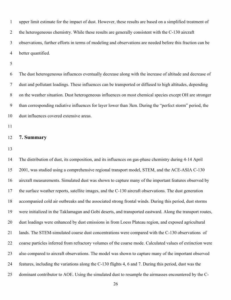
7. Summary 12

13

The distribution of dust, its composition, and its influences on gas-phase chemistry during 4-14 April 14

2001, was studied using a comprehensive regional transport model, STEM, and the ACE-ASIA C-130 15

aircraft measurements. Simulated dust was shown to capture many of the important features observed by 16

the surface weather reports, satellite images, and the C-130 aircraft observations. The dust generation 17

accompanied cold air outbreaks and the associated strong frontal winds. During this period, dust storms 18

were initialized in the Taklamagan and Gobi deserts, and transported eastward. Along the transport routes, 19

dust loadings were enhanced by dust emissions in from Loess Plateau region, and exposed agricultural 20

lands. The STEM-simulated coarse dust concentrations were compared with the C-130 observations of 21

coarse particles inferred from refractory volumes of the coarse mode. Calculated values of extinction were 22

also compared to aircraft observations. The model was shown to capture many of the important observed 23

features, including the variations along the C-130 flights 4, 6 and 7. During this period, dust was the 24

dominant contributor to AOE. Using the simulated dust to resample the airmasses encountered by the C-25

27

130 flights, and to divide them into dust and non-dust events, the dusty air-masses were shown to have 1

elevated values of ∆Ca/∆Mg, −+ ∆∆ 244 / SONH , and ∆NO3

-/∆CO. 2

3

Dust influences on regional gas-phase chemistry can be classified into heterogeneous influences and 4

radiative influences, and both were studied. In this paper we introduced four heterogeneous reactions 5

involving O3, NO2, SO2 and HNO3 reactions on dusts. The C-130 flight 6 was significantly affected by 6

heterogeneous and radiative influences. The O3 heterogeneous uptake on dust had a significant impact on 7

flight 6, accounting for a 20 ppbv decrease in ozone levels. Only when this reaction was included in the 8

model were we able to represent the observed values. This reaction was shown to cause a broad decrease 9

in background O3. In polluted areas, this low O3 background reduced NO2 production, but caused NO 10

enhancement. The impact of the O3 heterogeneous loss on NO2 was usually stronger than that due to the 11

direct NO2 reaction on dust. As a result of these reactions HONO levels increased by up to 30% in some 12

polluted areas. The radiative influence of dust on photochemistry was largest for HOx. For ozone, 13

radiative influence of aerosols was large, but the contribution due to dust was not as strong as the 14

influences of the heterogeneous reactions. 15

16

The presence of dust was also shown to enhance sulfate production by 10 to 40% in dust rich regions, and 17

to result in an increase in the sulfate mass in the coarse fraction. The observational data also found similar 18

amounts of coarse mode-sulfate. A pathway for producing coarse-mode sulfate has important implications 19

for climate. Sulfate in the coarse-mode has a much weaker influence on radiative forcing than sulfate in 20

the fine-mode. Sulfate-on-dust, in comparison with sulfate-in-accumulation mode, scatters vastly less 21

solar energy, has a much shorter atmospheric life-time, and has a smaller impact on cloud-droplet number. 22

The results presented here provide an upper-limit estimate of the importance of this reaction pathway, 23

since the evaluation was done under high-dust load conditions. For individual events, as much as 30-40% 24

of the sulfate was found in the coarse-mode. When averaged over the 10 day period encompassing the 25

28

life-cycle of this large dust outbreak, 10-15% of sulfate was predicted in the coarse-mode over vast 1

regions downwind of the high sulfur emission regions of east Asia. 2

3

Reactions involving NO2 and nitric acid were shown to result in the accumulation of nitrate into the 4

aerosol, and this occurs mainly in the coarse mode (however, appreciable amounts may also appear in the 5

fine mode). 6

7

Clearly further work is needed to quantify the influences of dust in the photochemical and biogeochemical 8

cycles in East Asia. The heterogeneous reactions as modeled were very simple. More detailed 9

considerations of the possible effects of surface saturation, as well as competition for reactions on other 10

surfaces such as BC need to be considered. These effects, as well as a comprehensive comparison of 11

across the ACE-ASIA measurements are the subjects of a future paper. 12

13 These results also point out the challenges that the community faces in quantifying the impacts of aerosols 14

on the chemistry of the atmosphere. For example, the results presented here strongly suggest that 15

heterogeneous reactions involving dust and ozone can be important. However, quantifying the role of this 16

reaction in the field is challenging, as the ozone reaction with dust leaves no obvious signature on the 17

aerosol surface confirming that the reaction indeed occurred. Thus at present we must rely on inferring its 18

importance from changes in ambient levels of ozone, which requires de-convoluting the heterogeneous 19

reaction signal from competing gas-phase photochemical destruction/production reactions, along with 20

transport and deposition processes. 21

22

Furthermore the evaluation of the importance of heterogeneous reactions involving dust requires 23

quantification of the dust amount, its size and surface area distributions in space and time, and its 24

elemental composition. Of particular importance in understanding the mechanisms of these heterogeneous 25

29

reactions, and in evaluating our capabilities of modeling the phenomena, is the quantification of the 1

chemical composition of the aerosol over the entire size range that dust exists in the atmosphere. The 2

observations obtained during ACE-ASIA have produced the most comprehensive characterization of dust 3

to date. For example, the data on board the C-130 on dust mass (estimated from the refractory portion of 4

super-micron optical size distribution), mid-visible, low-RH light extinction by aerosols, along with 5

aerosol chemical composition data provided by PILS, TAS and MOI, discussed in this paper provide 6

valuable new information that imply and confirm aspects of the nature of the dust/pollution interactions in 7

the East Asia troposphere. However, the integration of these observations into a consistent data set that 8

can be used to quantify important aspects of dust pollution interaction (for example the amount of non-sea 9

salt sulfate in the coarse mode), and that can be used to test and constrain models remains a challenge. 10

Uncertainties in aspects of the observations (e.g., converting optical quantities to mass (associated with 11

composition and shape effects), and differences in the amount of information (for example temporal 12

resolution) on the chemical composition of the coarse and fine modes, provide ample opportunity for the 13

model, with over-simplified treatments of aerosol interactions, to “agree” with the observations. A closer 14

integration of the measurements and models, and the identification of additional indicators of 15

dust/chemistry interactions that can be used to more rigorously test/constrain models are needed. 16

17

18 19 Acknowledgements: 20 21 This work was supported in part by grants from the NSF Atmospheric Chemistry Program, NSF grant 22 Atm-0002698, NASA GTE and ACMAP programs, and the Department of Energy Atmospheric 23 Chemistry Program. This work (I. Uno) was also partly supported by Research and Development 24 Applying Advanced Computational Science and Technology (ACT-JST) and the CREST of Japan 25 Science and Technology Corporation. 26 27

Reference: 28

30

Anderson, T. L., S. J. Masonis, D. S. Covert, N. C. Ahlquist, S. G. Howell, A. D. Clarke, and C. S. 1 McNaughton, Variability of aerosol optical properties derived from in situ aircraft measurements 2 during ACE-Asia, J. Geophys. Res., 10.1029/2002JD003247, this issue. 3

Calvert, J. G., G. Yarwood, and A. M. Dunker, An evaluation of the mechanism of nitrous-acid formation 4 in the urban atmosphere, Research on Chemical Intermediates, 20 (3-5): 463-502, 1994. 5

Carter, W., Documentation of the SAPRC-99 chemical mechanism for voc reactivity assessment, Final 6 Report to California Air Resources Board Contract No. 92-329, University of California-7 Riverside, May 8, 2000 8

Carmichael, G. R., Y. Tang, G. Kurata, I. Uno, D. G. Streets, J.- H. Woo, H. Huang, J. Yienger, B. Lefer, 9 R. E. Shetter, D. R. Blake, A. Fried, E. Apel, F. Eisele, C. Cantrell, M. A. Avery, J. D. Barrick, 10 G.W. Sachse, W. L. Brune, S. T. Sandholm, Y. Kondo, H. B. Singh, R. W. Talbot, A. Bandy, A. 11 D. Clarke, and B. G. Heikes, Regional-Scale chemical transport modeling in support of intensive 12 field experiments: overview and analysis of the TRACE-P Observations, J. Geophys. Res., 13 10.1029/2002JD003117, 2003. 14

Clarke, A. D., Y. Shinozuka, V.N. Kapustin, S. Howell, B. Huebert, S. Masonis, T. Anderson, D. Covert, 15 R. Weber, J. Anderson, H. Zin, K.G. Moore II, and C. McNaughton, Size-distributions and 16 mixtures of black carbon and dust aerosol in Asian outflow: physio-chemistry, optical properties, 17 and implications for CCN, (submitted to J. Geophys. Res., this issue). 18

Conant, W. C., J. H. Seinfeld, J. Wang, G. R. Carmichael, Y. Tang, I. Uno, P. J. Flatau, K. M. 19 Markowicz, and P. K. Quinn, A model for the radiative forcing during ACE-Asia derived from 20 CIRPAS Twin Otter and R/V Ronald H. Brown data and comparison with observations, J. 21 Geophys. Res., this issue (in press). 22

Dentener, F. J., G. R. Carmichael, Y. Zhang, J. Lelieveld, and P. J. Crutzen, Role of mineral aerosol as a 23 reactive surface in the global troposphere, J. Geophys. Res., 101, 22869-22889, 1996. 24

Goodman, A. L., G. M. Underwood, and V. H. Grassian, A laboratory study of the heterogeneous reaction 25 of nitric acid on calcium carbonate particles, J. Geophys. Res., 105, 29053-29064, 2000. 26

Goodman, A. L., P. Li, C. R. Usher, and V. H. Grassian, Heterogeneous uptake of sulfur dioxide On 27 aluminum and magnesium oxide particles, J. Phys. Chem. A, 105, 6109-6120, 2001. 28

Grassian, V. H. , Chemical reactions of nitrogen oxides on the surface of oxide, carbonate, soot and 29 mineral dust particles: Implications for the chemical balance of the troposphere, J. Phys. Chem. A, 30 106, 860-877, 2002. 31

Hanisch, F. and J. N. Crowley, Heterogeneous reactivity of gaseous nitric acid on Al2O3, CaCO3, and 32 atmospheric dust samples: A Knudsen cell study, J. Phys. Chem. A, 105, 3096-3106, 2001. 33

Hess, M., P. Koepke, and I. Schult, Optical properties of aerosols and clouds: the software package 34 OPAC, Bulletin of the American Meteorological Society, 79(5), 831-844, 1998. 35

Huebert, B. J., T. Bates, P. B. Russell, G. Shi, Y. J. Kim, K. Kawamura, G. R. Carmichael, and T. 36 Nakajima, An overview of ACE-ASIA: strategies for quantifying the relationships between Asian 37 aerosols and their climatic impacts. (submitted to J. Geophys. Res., this issue). 38

Jacob, D. J., Heterogeneous chemistry and tropospheric ozone, Atmos. Environ., 34, 2131-2159, 2000. 39 Jordan, C. E., J. E. Dibb, B. E. Anderson , and H. E. Fuelberg, Uptake of nitrate and sulfate on dust 40

aerosols during TRACE-P. (submitted to J. Geophys. Res., TRACE-P issue), 2003. 41 Krueger, B. J., V. H. Grassian, A. Laskin, and J. P. Cowin, The transformation of solid atmospheric 42

particles into liquid droplets through heterogeneous chemistry: laboratory insights into the 43 processing of calcium containing mineral dust aerosol in the troposphere, submitted to Geophys. 44 Res. Letts., 30, 48-1 to 48-4. (DOI 10.1029/2002GL016563), 2003. 45

Lee, Y. N., R. Weber, Y. Ma, D. Orsini, K. Maxwell, D. Blake, S. Meinardi, G. Sachse, C. Harward, T. 46 Anderson, S. Masonis, A. D. Clarke, K. Moore, V. N. Kapustin, T.-Y. Chen, D. C. Thornton, F. H. 47 Tu, and A. R. Bandy, Airborne measurement of inorganic ionic components of fine aerosol 48 particles using the PILS-IC technique during ACE-ASIA and TRACE-P. (submitted to J. 49 Geophys. Res., this issue). 50

31

Liu, M. and D. L. Westpal, A study of the sensitivity of Simulated mineral dust production to model 1 resolution, J. Geophys. Res., 106 (D16), 18099-18112, 2001. 2

Madronich, S. and S. Flocke, The role of solar radiation in atmospheric chemistry, in Handbook of 3 Environmental Chemistry (P. Boule, ed.), Springer-Verlag, Heidelberg, 1-26, 1999. 4

Madronich, S., photodissociation in the atmosphere 1: actinic flux and the effects of ground reflections 5 and clouds, J. Geophys. Res., 92(D8), 9740-9752, 1987. 6

Monahan, E. C., D. E. Spiel, and K. L. Davidson, Amodel of marine aerosol generation via whitecaps and 7 wave disruption, Oceanic Whitecaps edited by E. C. Monahan and G. MacNiocaill, 167-174, D. 8 Reidel, Norwell, Mass., 1986. 9

Michel, A. E., C. R.Usher, and V. H. Grassian, Heterogeneous and catalytic uptake of ozone on mineral 10 oxides and dust: a knudsen cell investigation, Geophys. Res. Letts., 29, 10-1 to 10-4, 2002. 11

Phadnis, M. J., and G. R. Carmichael, Influence of mineral aerosol on the tropospheric chemistry of east 12 Asia, J. Atmos. Chem., 36, 285-323, 2000. 13

Prince, A. P., J. L. Wade, V. H. Grassian, P. D. Kleiber, and M. A Young, Heterogeneous reactions of 14 soot aerosols with nitrogen dioxide and nitric acid studied in an atmospheric chamber, Atmos. 15 Environ., 36, 5729-5740, 2002. 16

Redemann, J., S. J. Masonis, B. Schmid, T. L. Anderson, P. Russell, J. Livingston, A. Clarke, S. Howell, 17 and C. McNaughton, Clear-column closure studies of aerosol extinction and optical depth aboard 18 the NCAR C-130 in ACE-Asia, 2001. (submitted to J. Geophys. Res., this issue). 19

Song, C. H., and G. R. Carmichael, A three-dimensional modeling investigation of the evolution 20 processes of dust and sea-salt particles in east Asia, J. Geophys. Res., 106, 18,131-18, 154, 2001. 21

Streets, D. G., T.C. Bond, G. R. Carmichael, S. D. Fernandes, Q. Fu, D. He, Z. Klimont, S. M. Nelson, N. 22 Y. Tsai, M. Q. Wang, J.-H. Woo, and K. F. Yarber, A year-2000 inventory of gaseous and primary 23 aerosol emissions in Asia to support TRACE-P modeling and analysis (submitted to J. Geophys. 24 Res., TRACE-P issue), 2003. 25

Sun, J., M. Zhang, and L. Tungsheng, Spatial and temporal characteristics of dust storms in China and its 26 surrounding regions, 1960-1999: Relations to source area and climate, J. Geophys. Res., 106, 27 10325-10333, 2001. 28

Tang, Y., G. R. Carmichael, I. Uno, J.-H. Woo, G. Kurata, B. Lefer, R. E. Shetter, H. Huang, B. E. 29 Anderson, M. A. Avery, A. D. Clarke and D. R. Blake, Impacts of aerosols and clouds on 30 photolysis frequencies and photochemistry during TRACE-P, part II: three-dimensional study 31 using a regional chemical transport model, J. Geophys. Res., 10.1029/2002JD003100, 2003a. 32

Tang, Y., G. R. Carmichael, J.-H. Woo, N. Thongboonchoo, G. Kurata, I. Uno, D. G. Streets, D. R. 33 Blake, R. J. Weber, R. W. Talbot, Y. Kondo and H. B. Singh, the influences of biomass burning 34 during TRACE-P experiment identified by the regional chemical transport model, J. Geophys. 35 Res., 10.1029/2002JD003110, 2003b. 36

Underwood, G. M., C. H. Song, M. Phadnis, G. R. Carmichael, and V. H. Grassian, Heterogeneous 37 reactions of NO2 and HNO3 on oxides and mineral dust: A combined laboratory and modeling 38 study, J. Geophys. Res., 106, 18,055-18,066, 2001. 39

Uno, I., G. R. Carmicahel, D.G. Streets, Y. Tang, J. J. Yienger, S. Satake, Z. Wang, J.-H. Woo, S. 40 Guttikunda, M. Uematsu, K. Matsumoto, H. Tanimoto, K. Yoshioka and T. Iida, Regional 41 Chemical Weather Forecasting System CFORS: Model descriptions and analysis of surface 42 observations at Japanese island stations during the ACE-ASIA experiment. (submitted to J. 43 Geophys. Res., this issue). 44

Usher, C. R., H. Al-Hosney, S. Carlos-Cuellar, and V. H. Grassian, A laboratory study of the 45 heterogeneous uptake and oxidation of sulfur dioxide on mineral dust particles, J. Geophys. Res., 46 107 (D23): art. no. 4713, 2002, 47

Wang, T., A. J. Ding, D. R. Blake, W. Zahorowski, C. N. Poon, and Y. S. Li, Chemical Characterization 48 of the Boundary Layer Outflow of Air Pollution to Hong Kong during February- April 2001, 49 (submitted to J. Geophys. Res., TRACE-P issue), 2003. 50

32

Woo, J.-H., D. G. Streets, G. R.Carmichael, Y. Tang, B.-I. Yoo, W.-C. Lee, N. Thongboonchoo, S. 1 Pinnock, G. Kurata, and I. Uno, Biomass and Biofuel Emissions and Their Impact on Trace Gas 2 Distributions in Asia during the TRACE-P Experiment, J. Geophys. Res., 10.1029/2002JD003200, 3 2003. 4

Zhang, X. Y., J. J. Cao, L. M. Li, R. Arimoto, Y. Cheng, B. Huebert, and D. Wang, characterization of 5 atmospheric aerosol over XiAn in south margin of Loess Plateau, China, Atmos. Environ., 26, 6 4189-4199, 2002. 7

Zhang, Y. and G. R. Carmichael, The role of mineral aerosol in tropospheric chemistry in East Asia – A 8 model study, J. Apply. Meteoro., 38, 353-366, 1999. 9

10

33

Table 1. Reaction index as mentioned in Figure 9.

Reaction Index # Reaction Equations

1 NO2 + hv → NO + O3P 2 O3P + O2 → O3 7 O3 + NO → NO2 + O2 8 O3 + NO2 → NO3 + O2 9 NO + NO3 → 2NO2 17 O3 + hv → O2 + O3P 18 O3 + hv → O2 + O1D 19 O1D + H2O → 2OH 21 OH + NO → HONO 22 HONO + hv → OH + NO 25 OH + NO2 → HNO3 29 OH + CO + O2 → HO2 + CO2 30 OH + O3 → HO2 + O2 31 HO2 + NO → NO2 + OH 32 HO2 + NO2 → HNO4 41 H2O2 + hv → 2OH 44 OH + SO2 + H2O + O2 → H2SO4 + HO2 125 OH + HCHO → HO2 + CO 236 NO2 + Dust → 0.5Nitrate + 0.5 Nitrite 237 O3 + Dust → 1.5O2

34

Figure Captions: Figure 1. STEM schematic for considering the aerosol impacts on photolysis rates as well as heterogeneous chemistry. Figure 2. Dust storms shown by the model simulation, surface synoptic observation, and GMS-5 satellite images (dust enhanced) at 06GMT (about 14:00 local time) of April 7, 9, and 11. The model results (left plates) are averaged from the model layers below 3km, and dust symbols are plotted in the station locations where dust weathers were reported at those times. The path (red line) of C-130 flight 6 is shown on plot C. Figure 3. Simulated and observed coarse dust and total aerosol optical extinction (AOE) along C-130 flights 4, 6, and 7. The modeled coarse dust concentrations are compared to the volume concentration of observed coarse particles whose evaporative temperature is higher than 300°C. The error bars in right plots are equal to 50% of modeled dust AOE, which represents the possible estimation error due to irregular dust shape and size. Figure 4. Observed correlations among PILS sub-micron ions and CO during C-130 flights 2 to 17 for dust and non-dust events in west of longtitude130E. Dust events were defined as that modeled total dusts were higher than 100 ug/m3 in standard state, and non-dust events were defined as that these concentrations were lower than 1 ug/m3. The linear best-fit lines and correlation coefficients R are marked in the plots. Figure 5. Observed aerosol compositions (A) and optical properties (B) during C-130 flight 6. Figure 6. Observed and simulated O3, SO2, CO, ethyne concentrations, and simulated J[O3→O2+O1D] and OH, along the path of the C-130 flight 6 (April 11). The three simulations (NORMAL, NODUST and FULL) have the nearly same concentrations for CO and ethyne. Figure 7. Trajectory paths that arrived at the C-130 flight path at 2:20GMT (A) (solid line) and 3:17GMT (B) (dashed line), April 11. Figure 8. Extracted results from the three simulations along the trajectory path A in Figure 7. A) O3 concentrations, altitude in AGL (altitude above ground level), and longitude. B) O3 budgets and O3 heterogeneous loss rate on dust (all loss terms are shown in negative values, same as below). C) NO2 concentrations and NO2 heterogeneous loss rate on dust. D) NO concentrations and the loss via reaction NO + O3 → NO2 + O2. E) SO2 concentrations and SO2 heterogeneous loss rate on dust. F) HNO3 concentrations and HNO3 heterogeneous loss rate on dust. G) OH concentrations. H) HONO/NO2 along the trajectory path. I) O3 difference between FULL and NORMAL simulations versus O3 heterogeneous loss rate on dust for all the points along the trajectory A. Figure 9. The chemical budgets and their main components for O3, NO2, NO, and OH when the trajectory path A (Figure 7) passed over Beijing at Julian day 100.14 (Figure 8), or 11:20 local time, April 10. Some small budgets and terms are multiplied with 10 or 100 for displaying purpose. All loss terms are presented in negative value. For each term, the bar sequence from left to right are in FULL, NORMAL and NODUST. The reaction index (R#) is listed in Table 1.

35

Figure 10. Extracted results from the three simulations along the trajectory path B in Figure 7. A) O3 concentrations, altitude, and O3 heterogeneous loss rate on dust. B) O3 difference between FULL and NORMAL simulations versus O3 heterogeneous loss rate on dust for all the points along the trajectory B. Figure 11. Averaged dust influences ((NORMAL-NODUST)/NODUST×100%) on O3 and daytime OH via changing photolysis rates, represented in percentage change, for the layers below 1km, 1 to 3km during the period from April 4 to 14. Figure 12. Averaged dust influences ((FULL-NORMAL)/NORMAL×100%) on O3, NO2, SO2, and HNO3 below 1km via the heterogeneous reactions for the period April 4-14. Figure 13. Same as Figure 12 but for daytime OH, NO, HONO, and sulfate.

Aerosols Sea salt, BC, OC, Dust,

other PM2.5, other PM10

Heterogeneous Reactions

Cloud fieldDobson O3

On-line TUV

Aerosol Optical

Properties

Gas-phase absorption

Tropospheric O 3

Gas-phase SpeciesSAPRC-99 Reactions

Photolysis Rates

Figure 1.

Simulated Dust Concentration (ug/m3) Averaged in the layers below 3km

Figure 2.

06GMT, April 07, 2001

06GMT, April 09, 2001

06GMT, April 11, 2001

A)

B)

C)

C-130 #6

0 2 4 6 8 10TIME (GMT)

0

20

40

60

80

100

Coa

rse

Dus

t (u

g/st

d m

3 )

0

2000

4000

6000

8000

Flig

ht A

ltitu

de (m

)

Observed Coarse ParticleSimulated Coarse DustFlight Altitude

Observed and Simulated Dust in C-130 Flight #4 (04/06/2001)

0 2 4 6 8 10

TIME (GMT)

0

4E-005

8E-005

0.00012

0.00016

AO

E @

550

nm (/

m)

0

2000

4000

6000

8000

Flig

ht A

ltitu

de (m

)

Observed AOESimulated AOE with DustSimulated AOE without DustFlight Altitude

Observed and Simulated AOE in C-130 Flight #4 (04/06/2001)

0 2 4 6 8TIME (GMT)

0

500

1000

1500

2000

2500

Coa

rse

Dus

t (u

g/st

d m

3 )

0

2000

4000

6000

8000F

light

Alt

itud

e (m

)

Observed Coarse ParticleSimulated Coarse DustFlight Altitude

Observed and Simulated Dust in C-130 Flight #6 (04/11/2001)

0 2 4 6 8

TIME (GMT)

0

0.0002

0.0004

0.0006

0.0008

AO

E @

550

nm (/

m)

0

2000

4000

6000

8000

Flig

ht A

ltitu

de (m

)

Observed AOESimulated AOE with DustSimulated AOE without DustFlight Altitude

Observed and Simulated AOE in C-130 Flight #6 (04/11/2001)

0 2 4 6 8 10TIME (GMT)

0

400

800

1200

1600

Coa

rse

Dus

t (u

g/st

d m

3 )

0

2000

4000

6000

8000

Flig

ht A

ltit

ude

(m)

Observed Coarse ParticleSimulated Coarse DustFlight Altitude

Observed and Simulated Dust in C-130 Flight #7 (04/12/2001)

0 2 4 6 8 10

TIME (GMT)

0

0.0001

0.0002

0.0003

0.0004

0.0005

AO

E @

550

nm (/

m)

0

2000

4000

6000

8000

Flig

ht A

ltitu

de (m

)

Observed AOESimulated AOE with DustSimulated AOE without DustFlight Altitude

Observed and Simulated AOE in C-130 Flight #7 (04/12/2001)

Figure 3.

Figure 4.

A) B)

C) D)

E) F)

0 2 4 6 8

TIME (GMT)

0

4

8

12

16

20

Obs

erve

d A

eros

ol C

ompo

sitio

ns (

ug/s

td m

3 )

0

2000

4000

6000

8000

Alt

itud

e (m

)

PILS SulfatePILS NitratePILS CaPILS NH4

0

0.2

0.4

0.6

0.8M

OI

Coa

rse

Fra

ctio

n

MOI Coarse CaMOI Sulfate Coarse FractionMOI Nitrate Coarse FractionFlight Altitude

0 2 4 6 8TIME (GMT)

0

1E-005

2E-005

3E-005

4E-005

5E-005

Tot

al A

bsor

ptio

n @

550

nm (1

/m)

0

2000

4000

6000

8000

Alti

tud

e (m

)

Total AbsorptionTotal ScatteringFine Fraction of AbsorptionFine Fraction of ScatteringFlight Altitude

0

0.0002

0.0004

0.0006

0.0008

Tot

al S

catt

erin

g @

550

nm (1

/m)

0

0.2

0.4

0.6

0.8

1

Subm

irco

n Fr

actio

n

Figure 5.

A)

B)

0 2 4 6 8TIME (GMT)

20

30

40

50

60

70

80

O3 (

ppbv

)

0

2000

4000

6000

8000

Alti

tude

(m)

ObservedNORMALNODUSTFULLFlight Altitude

0 2 4 6 8

TIME (GMT)

0

4

8

12

SO2 (

ppbv

)

0

2000

4000

6000

8000

Alti

tude

(m)

ObservedNORMALNODUSTFULLFlight Altitude

0 2 4 6 8

TIME (GMT)

100

200

300

400

500

600

CO

(ppb

v)

0

2000

4000

6000

8000

Alt

itud

e (m

)

ObservedNORMALNODUSTFULLFlight Altitude

0 2 4 6 8

TIME (GMT)

0

0.5

1

1.5

2

2.5

Eth

yne

(ppb

v)

0

2000

4000

6000

8000

Alti

tud

e (m

)

ObservedNORMALNODUSTFULLFlight Altitude

0 2 4 6 8TIME (GMT)

0

1E-005

2E-005

3E-005

4E-005

5E-005

J[O

3 =>

O2+

O(1 D

)]

0

2000

4000

6000

8000

Alti

tud

e (m

)

NORMALNODUSTFlight Altitude

0 2 4 6 8

TIME (GMT)

0

5E-005

0.0001

0.00015

0.0002

0.00025

OH

(ppb

v)

0

2000

4000

6000

8000

Alti

tud

e (m

)

NORMALNODUSTFULLFlight Altitude

Figure 6.

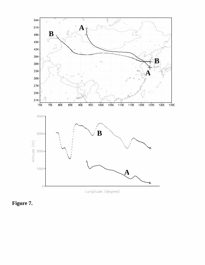
Figure 7.

AB

B

A

A

B

98 98.5 99 99.5 100 100.5 101 101.5

Julian Day (GMT)

20

30

40

50

60

70O

3 (p

pbv)

0

1000

2000

3000

4000

AG

L (m

)

NORMALNODUSTFULLAltitude (AGL)Longitude

90

100

110

120

130

Lon

gitu

de

98 98.5 99 99.5 100 100.5 101 101.5

Julian Day (GMT)

-0.002

-0.001

0

0.001

0.002

0.003

O3 B

udge

t (pp

bv/s

)

-0.0002

-0.00016

-0.00012

-8E-005

-4E-005

0

O3 L

oss

on D

ust (

ppbv

/s)

NORMALNODUSTFULLO3 Loss on Dust

98 98.5 99 99.5 100 100.5 101 101.5Julian Day (GMT)

0

2

4

6

NO

2 (pp

bv)

-4E-005

-3E-005

-2E-005

-1E-005

0

NO

2 Los

s on

Dus

t (pp

bv/s

)

NORMALNODUSTFULLNO2 Loss on Dust

98 98.5 99 99.5 100 100.5 101 101.5

Julian Day (GMT)

0

1

2

3

NO

(ppb

v)

NORMAL NONODUST NOFULL NONORMAL: NO+O3 =>NODUST: NO+O3=>FULL: NO+O3=>

-0.04

-0.03

-0.02

-0.01

0

NO

Los

s vi

a [N

O+O

3=>N

O2+

O2]

(ppb

v/s)

98 98.5 99 99.5 100 100.5 101 101.5Julian Day (GMT)

0

2

4

6

8

10

SO2 (

ppbv

)

-8E-005

-6E-005

-4E-005

-2E-005

0

SO2 L

oss

on D

ust (

ppbv

/s)

NORMALNODUSTFULLSO2 Loss on Dust

98 98.5 99 99.5 100 100.5 101 101.5

Julian Day (GMT)

0

0.5

1

1.5

2

2.5

HN

O3 (

ppbv

)

-0.00012

-8E-005

-4E-005

0

HN

O3 H

eter

ogen

eous

Los

s (p

pbv/

s)

NORMALNODUSTFULLHNO3 Budget in FULL

Figure 8 (continued on next Page)

A) B)

C) D)

E) F)

Figure 8 (continued)

98 98.5 99 99.5 100 100.5 101 101.5

Julian Day (GMT)

0

4E-005

8E-005

0.00012

0.00016

0.0002

OH

(ppb

v)

NORMALNODUSTFULL

98 98.5 99 99.5 100 100.5 101 101.5

Julian Day (GMT)

0

0.004

0.008

0.012

HO

NO

/NO

2

NORMALNODUSTFULL

-0.0002 -0.00016 -0.00012 -8E-005 -4E-005 0O3 Loss on Dust (ppbv/s)

-25

-20

-15

-10

-5

0

O3 D

iffe

renc

e (F

UL

L-N

OR

MA

L) (

ppbv

)

Fit Line: Y = 108033 * X - 0.21 R2=0.87

G) H)

I)

-0.04

-0.02

0

0.02

0.04

0.06O

3 Bud

get a

nd I

ts C

ompo

nent

s (p

pbv/

s)

FULLNORMALNODUST

10 x Net Budget

R#2

R#7

10 x R#8

R#17

10 x R#237

R#18

-0.04

-0.02

0

0.02

0.04

NO

2 Bud

get a

nd I

ts C

ompo

nent

s (p

pbv/

s)

FULLNORMALNODUST

10 x Net Budget

R #1

R #7

10 x R#8

10 x R#9

10 x R#25

10 x R#31

10 x R#32

100 x R#236

-0.04

-0.02

0

0.02

0.04

NO

Bud

get

and

Its

Com

pone

nts

(ppb

v/s)

FULLNORMALNODUST

10 x Net Budget

R#1

R#7

10 x R#9 10 x R#31

10 x R#51100 x R#21

-0.0002

-0.0001

0

0.0001

0.0002

0.0003

0.0004

0.0005

0.0006

OH

(ppb

v) a

nd I

ts B

udge

t Com

pone

nts

(ppb

v/s)

FULLNORMALNODUST

OH Concentrations

R#19

R#21

R#22

R#25R#29

R#30

R#31

10 x R#41

R#44 R#125

Figure 9.

A)

C)

B)

D)

97 97.5 98 98.5 99 99.5 100 100.5 101 101.5

Julian Day (GMT)

30

40

50

60

70

O3

(ppb

v)

2000

3000

4000

5000

6000

AG

L (m

)

NORMALNODUSTFULLAltitude (AGL)O3 Loss on Dust

-6E-005

-4E-005

-2E-005

0

O3 L

oss

on D

ust

(ppb

v/s)

-6E-005 -4E-005 -2E-005 0

O3 Loss on Dust (ppbv/s)

-16

-12

-8

-4

0

4

O3 D

iffer

ence

(FU

LL

-NO

RM

AL

) (pp

bv)

Fit Line: Y = 212846 * X - 0.0023 R2=0.98

Figure 10.

A) B)

Figure 11.

Influence on OH below 1km Influence on O3 below 1km

Influence on OH from 1 to 3km Influence on O3 from 1 to 3km

Average Dust Radiative Influence on Daytime OH (%)

Average Dust Radiative Influence on O3 (%)

Figure 12.

Heterogeneous Influence on O3 Heterogeneous Influence on NO2

Heterogeneous Influence on SO2 Heterogeneous Influence on HNO3

Averaged Dust Heterogeneous Influences (%) below 1km

Figure 13.

Heterogeneous Influence on Daytime OH Heterogeneous Influence on NO

Averaged Dust Heterogeneous Influences (%) below 1km

Heterogeneous Influence on HONO Heterogeneous Influence on Sulfate