1. The Basics of Survival Analysis

Special features of survival analysis

Censoring mechanisms

Basic functions and quantities in survival analysis

Models for survival analysis

§1.1. Special features of survival analysis

• Application fields of survival analysis

Medicine, Public health, Epidemiology, Engineering, etc.

• Time-to-event

The main variable of interest in survival analysis is time-to-event.

Time-to-event is a positive random variable.

Examples of time-to-event:

Times to death of patients with certain disease

Remission duration of certain disease in clinical trials

Incubation times of certain disease, such as AIDS, Hyper-

titis B, SARS etc.

Failure times of certain manufactured products

Life times of elderly in particular social programs

1

• Incomplete observation of time-to-event

Example 1.1. Survival time of HIV+ patients

Times-to-event are not always completely observable. These times

are subject to censoring and truncation. For a censored or a trun-

cated time-to-event, only partial information is available.

Types of censoring:

left censoring, right censoring, interval censoring.

Types of truncation:

left truncation, right truncation, interval truncation.

2

§1.2 Censoring mechanisms

• Right censoring

Right censoring includes ordinary type I censoring, progressive

type I censoring, generalized type I censoring, random censoring

and type II censoring. We will focus only on ordinary and gen-

eralized type I censoring and random censoring.

Ordinary Type I censoring:

The censoring time is prespecified and the same for all individuals.

this kind of censoring is usually used in animal studies and clinical

trials.

Figure 1.1 Illustration of ordinary Type I censoring

3

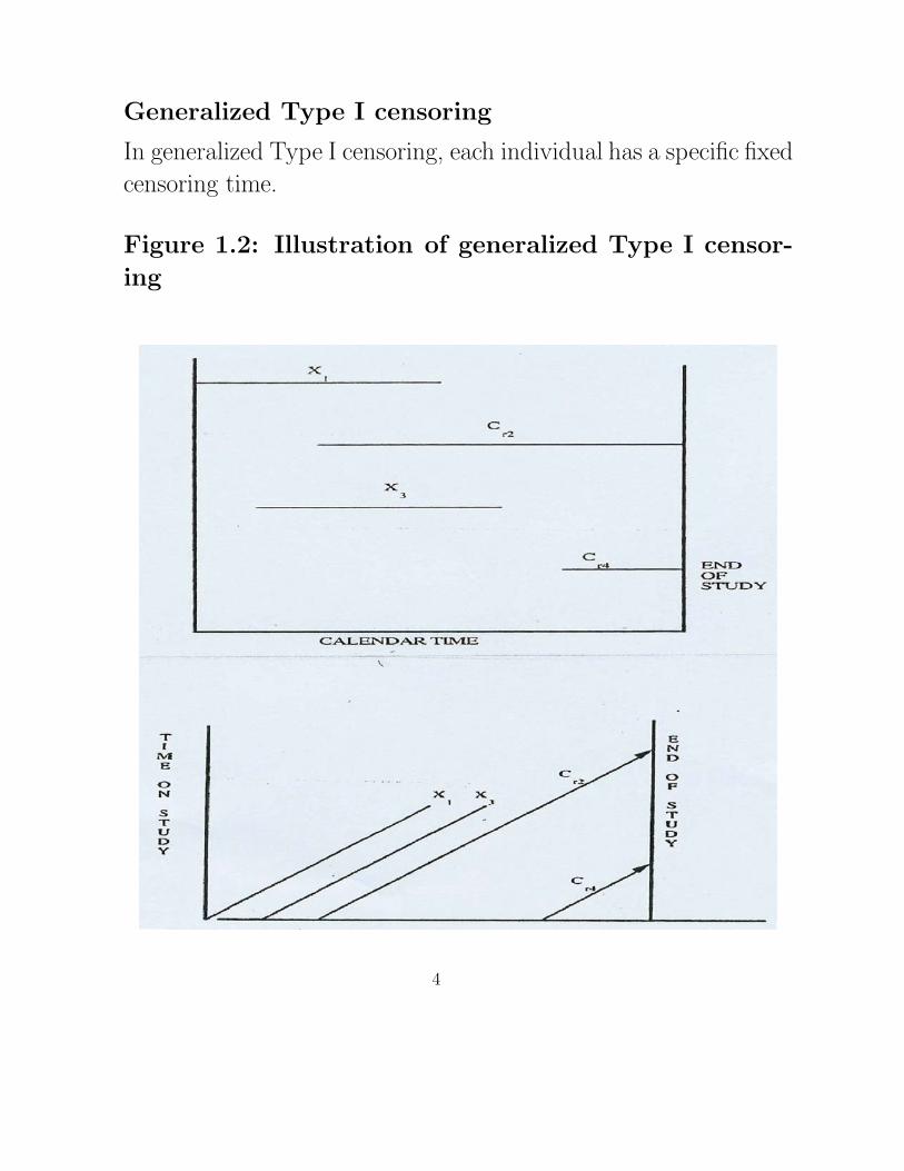
Generalized Type I censoring

In generalized Type I censoring, each individual has a specific fixed

censoring time.

Figure 1.2: Illustration of generalized Type I censor-

ing

4

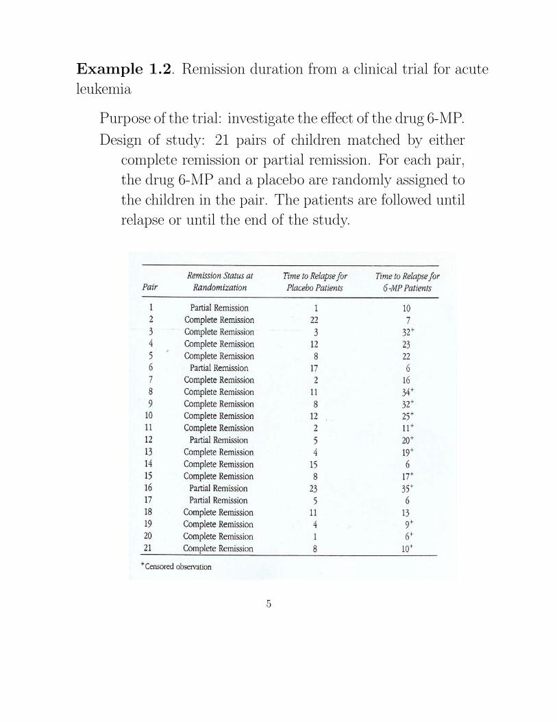
Example 1.2. Remission duration from a clinical trial for acute

leukemia

Purpose of the trial: investigate the effect of the drug 6-MP.

Design of study: 21 pairs of children matched by either

complete remission or partial remission. For each pair,

the drug 6-MP and a placebo are randomly assigned to

the children in the pair. The patients are followed until

relapse or until the end of the study.

5

• Random censoring

Each individual is censored at random.

Random censoring can be described by a random variable C which

is independent of X . An individual is censored if C < X .

• Left censoring

A lifetime X associated with an individual in a study is considered

to be left censored if it is less than a censoring time Cl. The data

observed on the individual can be recorded as (T, ε) where

T = max{X, Cl},ε =

{1, if T = X,

0, if T = Cl.

Example 1.3. Childhood learning

Time-to-event: the age at which a child learns to accom-

plish certain tasks in children learning centers.

Left censoring occurs if children can already perform the

tasks when they start their study at the centers.

6

Example 1.4. Time to first use of marijuana

Data are collected through survey by asking “When did

you first use marijuana?” The answers are:

a. Exact age

b. I never used it.

c. I used it but can not remember when the first

time was.

Answer c gives a left censored observation.

• Interval censoring

When lifetime is only known to fall within an interval, it is referred

to as interval censoring. Interval censoring occurs in clinical trial

where patients have periodic follow-ups, and in industrial experi-

ments where equipment items are inspected periodically, etc.

Example 1.5. Time to cosmetic deterioration of breast cancer

patients

To compare the cosmetic effect of two treatments on early

breast cancer patients: (i) radiotherapy and (ii) radio-

therapy plus chemotherapy, patients were observed in

intervals. The event of interest is the first time breast

retraction is obeserved.

7

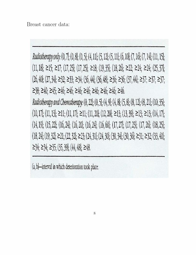
Breast cancer data:

8

• Truncation

Truncation is a different phenomenon from censoring. Truncation

is due to sampling bias that only those individuals whose lifetimes

lie within a certain interval [YL, YR] can be observed.

Left truncation YR = ∞.

Example 1.6. Death times of elderly residents of a retirement

community

The time a resident died or left the community is observed. The

entry time is recorded. Only the elderly people of a certain age

can be admitted into the community. People died before this age

can not be observed.

Right truncation YL = 0

Example 1.7. Time to AIDS

258 adults and 37 children who were infected with AIDS virus after

April 1, 1978 and developed AIDS by June 30 , 1986 were included

in a study. Those who were infected in this period but have not

yet developed AIDS are not observed

The event of interest is the induction time (period from time of

infection to time of onset of AIDS).

For people infected at a particular infection time, their induction

time is truncated at the length which equals the period from the

infection time to June 30 , 1986.

9

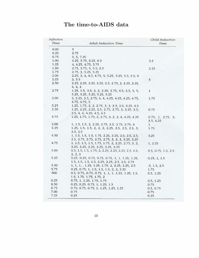
The time-to-AIDS data

10

§1.3. Basic functions and quantities in survival analysis

Let X denote the random variable time-to-event.

Besides the usual probability density function f (x) and cumulative

distribution function F (x), the distribution of X can be described by

several equivalent functions. They are:

Survival function, Hazard function, Cumulative hazard func-

tion, and so on.

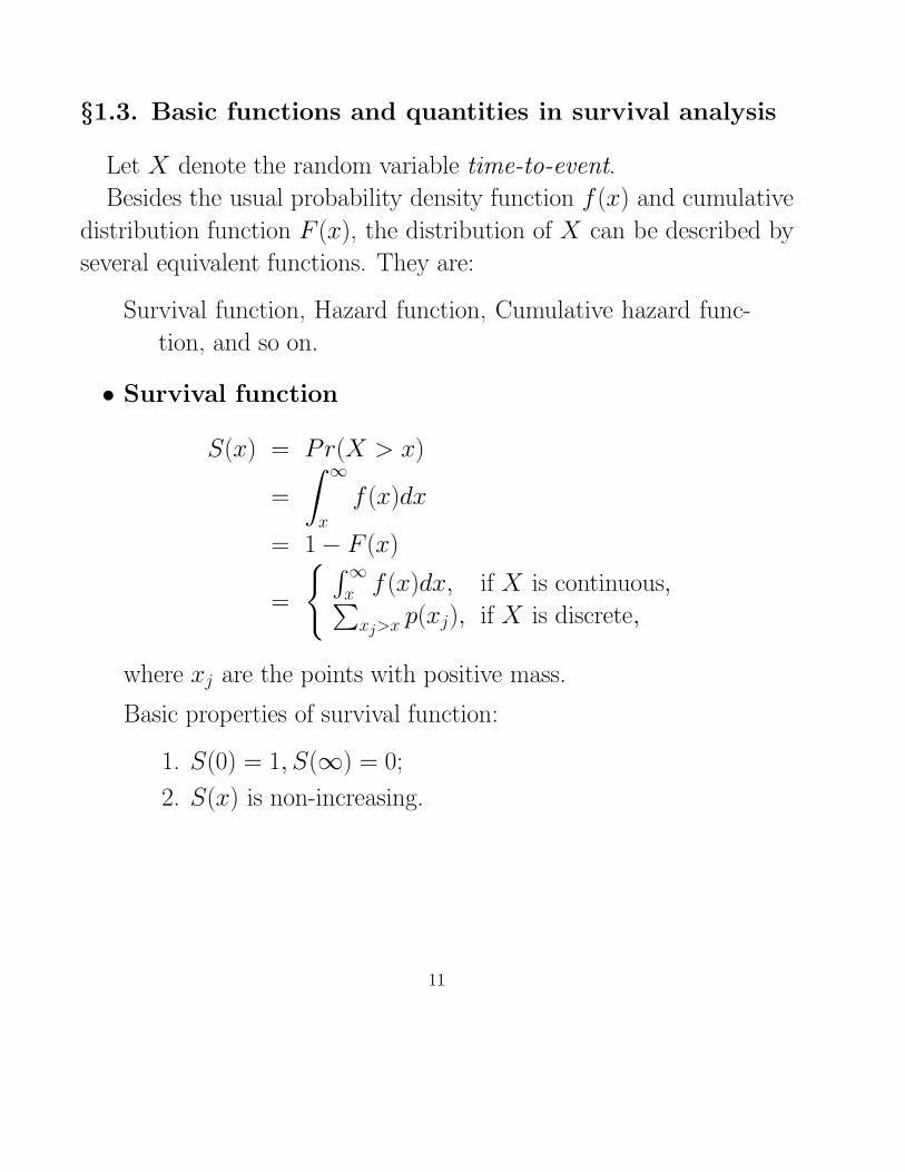
• Survival function

S(x) = Pr(X > x)

=

∫ ∞

x

f (x)dx

= 1 − F (x)

=

{ ∫ ∞x f (x)dx, if X is continuous,∑

xj>x p(xj), if X is discrete,

where xj are the points with positive mass.

Basic properties of survival function:

1. S(0) = 1, S(∞) = 0;

2. S(x) is non-increasing.

11

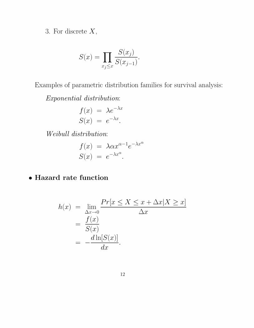
3. For discrete X ,

S(x) =∏xj≤x

S(xj)

S(xj−1).

Examples of parametric distribution families for survival analysis:

Exponential distribution:

f (x) = λe−λx

S(x) = e−λx.

Weibull distribution:

f (x) = λαxα−1e−λxα

S(x) = e−λxα.

• Hazard rate function

h(x) = lim∆x→0

Pr[x ≤ X ≤ x + ∆x|X ≥ x]

∆x

=f (x)

S(x)

= −d ln[S(x)]

dx.

12

The hazard rate function can be viewed as the probability of an

individual of age x experiencing the event instantateously.

Examples:

Exponential distribution:

h(x) = λ.

Weibull distribution:

h(x) = λαxα−1.

Generic types of hazard rates:

1. Constant

Un-realistic.

2. Increasing: Convex or concave

Arising from natural aging or wear

3. Decreasing: Convex or concave

Lifetimes of electronic devices; Patients experincing

certain types of transplants; etc.

4. Convex bathtub shape

Appropriate for populations followed from birth;

Mortality data; Manufactured equipments; etc.

5. Concave bump shape

Survival after successful surgery; etc.

13

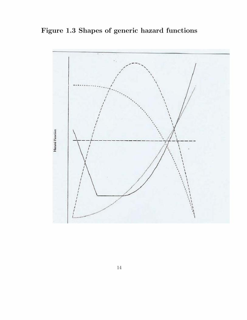
Figure 1.3 Shapes of generic hazard functions

14

• Cumulative hazard function

Continuous case:

H(x) =

∫ x

0

h(x)dx

=

∫ x

0

[−d ln[S(x)]

dx

]dx

= − ln[S(x)]

Discrete case:

H(x) =∑xj≤x

h(xj).

§1.4. Regression models for survival data

Regression models accounting for covariates which cause het-

erogeneity.

Covariates could be quantitative, e.g., blood pressure, temper-

ature, age, weight, etc.

Covariates could also be qualitative, e.g., gender, race, treat-

ment, disease status, etc.

Covariates may or may not be time-depedent. The covariates

are denoted by

Zt(x) = (Z1(x), . . . , Zp(x)).

15

• Log survival time regression

Let Y = ln(X). Y is modeles as

Y = µ + γ′Z + σW,

where W is a random variable with mean 0 and variance 1.

Choices of the distribution of W :

Normal — corresponding to log-normal distribution for X ,

Extreme-value — corresponding to Weibull distribution for

X ,

Logistic — corresponding to log-logistic distribution for X .

Survival function under the model:

S(x|Z) = Pr[X > x|Z] = Pr[Y > lnx|Z ]

= Pr[µ + σW > ln x − γ′Z|Z ]

= Pr[eµ+σW > x exp{−γ′Z}|Z]

= S0(x exp{−γ′Z}),

where S0 is the survival function of the baseline failure time

exp{µ + σW}. This model is called the accelerated failure-time

model, since the failure-time is accelerated by a factor exp{−γ′Z}.

Hazard function

h(x|Z) = h0(x exp{−γ′Z}) exp{−γ

′Z}.

16

Example:

Suppose W follows an extreme value distribution with density

function fW (w) = exp{w − ew}. Let Y = ln X = γ′Z + σW.

Then

S(x|Z) = S0(x exp(−γ′Z)) = exp{−[x exp(−γ

′Z)]1/σ}

h(x|Z) = h0(x exp(−γ′Z)) =

1

σ[x exp(−γ

′Z)]1/σ−1,

where S0(t) = e−t1/σand h0(t) = 1

σt1/σ−1 are the survival and

hazard functions of X0 = eW .

• Hazard rate regression

It is more flexible to model the hazard rate by a regression function

of the covariates.

Multiplicative hazard models

The hazard rate is modeled as

h(x|Z) = h0(x)c(β′Z),

where h0(x) is a baseline hazard function and c(·) is a positive

function.

The multiplicative model has the feature that, if all the covariates

are fixed at time zero, the hazard rates of two individuals with

different covariate values are proportional. It is easy to see that

h(x|Z1)

h(x|Z2)=

c(β′Z1)

c(β′Z2)

.

17

The survival function of the multiplicative hazard model:

S(x|Z) = S0(x)c(β′Z).

In the particular Cox proportional hazard rate model,

c(β′Z) = exp(β

′Z).

• A remark on the estimation

In principle, the regression models can be estimated by maximum

likelihood method. But, due to computational difficulties involved

by using the exact likelihood, certain alternatives will be considered

for the estimation in the light of likelihood principle.

18