1

TCOM 5143Telecommunications Analysis, Planning

and Design

Lecture 6

Network Design and Graph Theory: part 2

Shortest Path trees and Tours

2

Definition: Shortest path:

• Given a weighted graph G(V,E); i.e., each edge has a weight W(e), and two nodes u and v, the shortest path from u to v is a path P from u to v such that the total weight of edges in the path P is minimum.

• Shortest paths have the following “optimal nest” property: Every subpath of a shortest path is a shortest path (between its own endvertices).

3

Definition: Shortest path Tree

• Given a weighted graph G(V,E) and a specified node r in the graph (called root node), a shortest-path (spanning) tree T is a spanning tree of G such that for all v V, the unique path from r to v in T is a shortest path from r to v in G.

4

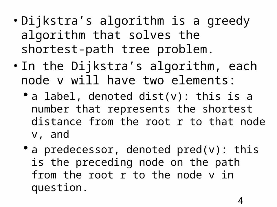
• Dijkstra’s algorithm is a greedy algorithm that solves the shortest-path tree problem.

• In the Dijkstra’s algorithm, each node v will have two elements: a label, denoted dist(v): this is a number that

represents the shortest distance from the root r to that node v, and

a predecessor, denoted pred(v): this is the preceding node on the path from the root r to the node v in question.

5

Dijkstra’s algorithm:

Step 1. Mark the root node r as scanned and set the label of the root r to zero and set its predecessor to itself. The root is the only node that is its own predecessor.

Step 2. Mark all nodes except the root in the graph as unscanned and set their labels to .

For each node v adjacent to the root, set the label of the node to the weight of edge between the root and the node; i.e, dist(v)=W(r,v). Set pred(v)=r.

6

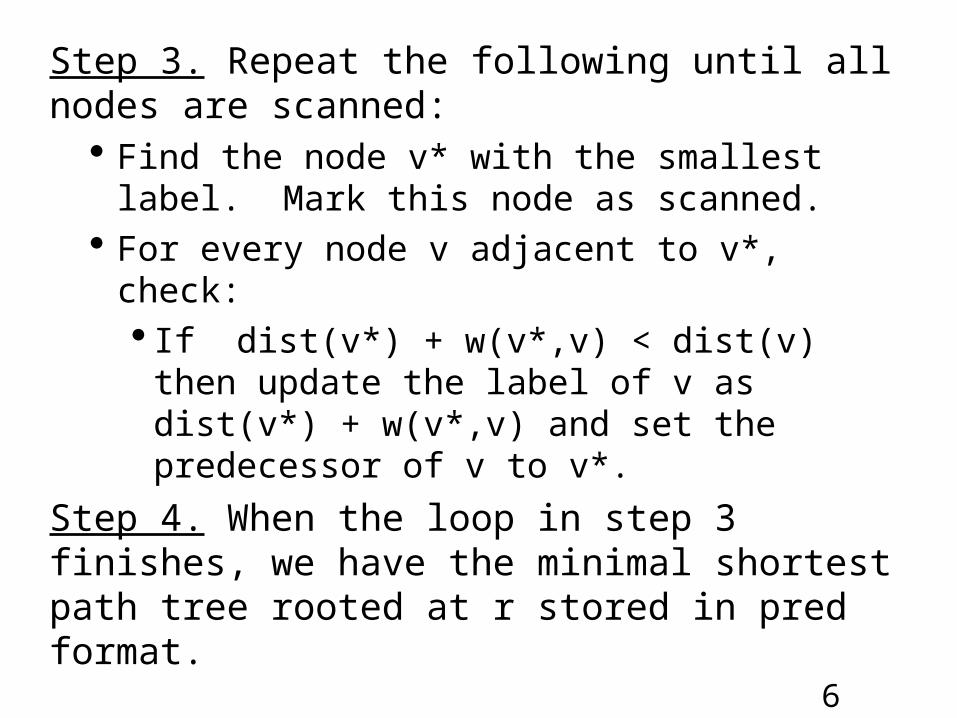
Step 3. Repeat the following until all nodes are scanned:

Find the node v* with the smallest label. Mark this node as scanned.

For every node v adjacent to v*, check: If dist(v*) + w(v*,v) < dist(v) then update the

label of v as dist(v*) + w(v*,v) and set the predecessor of v to v*.

Step 4. When the loop in step 3 finishes, we have the minimal shortest path tree rooted at r stored in pred format.

7

Notes:

• when the weights of all edges are positive, once a node is marked as scanned, then it need never be rescanned.

• If the label of a node changes, it must be rescanned.

8

Example:

• Find shortest paths from A to all other nodes in the graph below.

6

A

B

D

E

F

C

5

1 3

5

1

4

2

9

• Step 1 and 2:

Scanned nodes: A

• Step 3: v* is C because C has the lowest label. Scan C.

• So, scanned nodes are A,C

• Label of B becomes 4 because 3+1 < 5. And Pred(B)=C.

• Label of D becomes 6 because 5+1 < . And Pred(D)=C.

,

A

B

D

E

F

C

5

1 3

5

6

1

4

2

0,A

5,A

,

1,A ,

Label pred

10

• Step 3: Scan B because it has the lowest label (4).

• So, scanned nodes are A,B,C.

• The label of D becomes 5 (=4+1). Pred(D)=B

• The label of E becomes 10 (=4+6). Pred(E)=B

,

A

B

D

E

F

C

5

1 3

5

6

1

4

2

0,A

4,C

,

1,A 6,C

11

• Step 3: Scan D because it has the lowest label (5).

• So, the scanned nodes are A,B,C,D.

• Update the label of F as 9 (=5+4). And set pred(F)=D

10,B

A

B

D

E

F

C

5

1 3

5

6

1

4

2

0,A

4,C

,

1,A 5,B

12

• Step 3: Scan F because it has the lowest label 9.

• So, the scanned nodes are A,B,C,D,F..

• Do we update the label of E? no, because 9+2 is not < 10.

10,B

A

B

D

E

F

C

5

1 3

5

6

1

4

2

0,A

4,C

9,D

1,A 5,B

13

• Step 3: Scan E and we are done. The scanned nodes are A,B,C,D,E,F.

10,B

A

B

D

E

F

C

5

1 3

5

6

1

4

2

0,A

4,C

9,D

1,A 5,B

14

• The final solution is:

10,B

A

B

D

E

F

C

5

1 3

5

6

1

4

2

0,A

4,C

9,D

1,A 5,B

15

• The shortest path spanning tree for the example graph is therefore the following:

The tree is made of the six nodes connected with the large, blue links.

10,B

A

B

D

E

F

C

5

1 3

5

6

1

4

2

0,A

4,C

9,D

1,A 5,B

• In Delite, we can run Dijkstra’s algorithm by invoking Prim-Dijkstra from Delite with =1. ( is explained below.)

16

Comparing MSTs and SPTs: cost versus delay• Recall that for the 20-node MST in figure 3.4 in Cahn

textbook, the total link cost is $48,686/month, and its average delay over the network is

• The shortest-path spanning tree produced by Dijkstra’s algorithm in figure 3.7 in Cahn textbook is a star centered at the node N14. Its total link cost is $88,612/ month, and its average delay over the network is

• Note that in general the shortest-path spanning trees produced by Dijkstra’s algorithm are not stars.

901.0

ST*4158.4

099.01

ST*4158.4

981.0

ST*9000.1

019.01

ST*9.1

17

Tradeoffs between Total Link Cost and

• If we compare MSTs and SPTs (Shortest path trees), we find that MSTs have optimal (lowest) cost, but high average number of hops for large graph; SPTs do not have optimal (lowest) cost, but they have reasonable average number of hops for all graphs.

n-node MSTs(Kruskal’s; Prim’s)

n-node SPTs(Dijkstra’s)

Totalcost

optimal (lowest) non-optimal

hopshigh for large n reasonable forall n

hops

hops

18

Prim-Dijkstra Trees• One way to to produce designs that are not as

expensive as the SPTs or that are not associated with as high delays as the MSTs is to use the following labeling scheme in Dijkstra’s algorithm:

• Consider the scenario after the augmentation of the tree T (i.e., the vertex v has just been included), the update of label (u) for every neighbor u of v not in T is:

Prim’s label(u) = min {label(u), w(v, u)}

Dijkstra’s label(u) = min {label(u), label(v) + w(v, u)}.

19

Prim’s label(u) = min {label(u), w(v, u)}

Dijkstra’s label(u) = min {label(u), label(v) + w(v, u)}.

• A unified labeling scheme is

label(u) = min {label(u), label(v) + w(v, u)},

where [0, 1] is a parameter to yield the desired tradeoffs.

• For = 0, the unified algorithm reduces to Prim’s algorithm for MSTs.

• For = 1, the unified algorithm reduces to Dijkstra’s algorithm for shortest-path spanning trees.

20

• Table 3.12 in Cahn textbook shows a range of tradeoffs for a 100-node tree design over a range of -values in [0, 1].

hops link delay cost0.0 (MST)

0.10.20.30.40.50.60.70.80.9 (star)

13.947910.57177.86406.77625.66794.63033.70633.01862.28791.9800

0.30660.14510.10670.09130.07460.05980.04670.03800.02770.0233

$325,516$280,162$248,217$243,551$248,650$253,579$273,742$295,012$378,794$453,861

21

Comparing Candidate Designs: Dominance Among Designs

• Goal: Select the best designs based the following factors: network cost and performance (i.e., delay, reliability).

• Definition: For two candidate designs D1 and D2 with cost-performance (C1, P1) and (C2, P2), respectively, we say that D1 dominates D2 when

C1 < C2 and P1 is better than P2.

22

Notes:1. The interpretation of “P1 is better than P2” depends

on the context of performance: P1 < P2 when P measures network delay, whereas P1 > P2 when P measures network reliability.

2. The dominance relation, denoted by <, on a set S of candidate designs, is• irreflexive, i.e., for D S, D is not dominated by

D;• anti-symmetric, i.e., for D1, D2 S, D1 < D2 D2

is not < D1;• transitive, i.e., for D1, D2, D3 S, D1 < D2 and

D2 < D3 D1 < D3.

23

3.Two candidate designs D1 and D2 may not be comparable:

• D1 is not < D2 and D2 is not < D1,

that is, D1 and D2 exhibit a tradeoff in cost and performance.

24

The following table shows the dominance among the designs for the 100-node Prim-Disjksta trees

Design Dominates link delay costN0N1N2N3N4N5N6N7N8N9

noneN0N0,N1N0,N1,N2N0,N1N0,N1N0,N1N0nonenone

0.30660.14510.10670.09130.07460.05980.04670.03800.02770.0233

$325,516$280,162$248,217$243,551$248,650$253,579$273,742$295,012$378,794$453,861

25

• We should discard candidate designs N0, N1, and N2 because they are dominated by other candidates.

Design Dominates link delay costN3N4N5N6N7N8N9

N0,N1,N2N0,N1N0,N1N0,N1N0nonenone

0.09130.07460.05980.04670.03800.02770.0233

$243,551$248,650$253,579$273,742$295,012$378,794$453,861

• The remaining candidate designs are pairwise noncomparable candidate designs: They exhibit tradeoffs between cost and performance (delay). Each candidate can be used as a valid design.

26

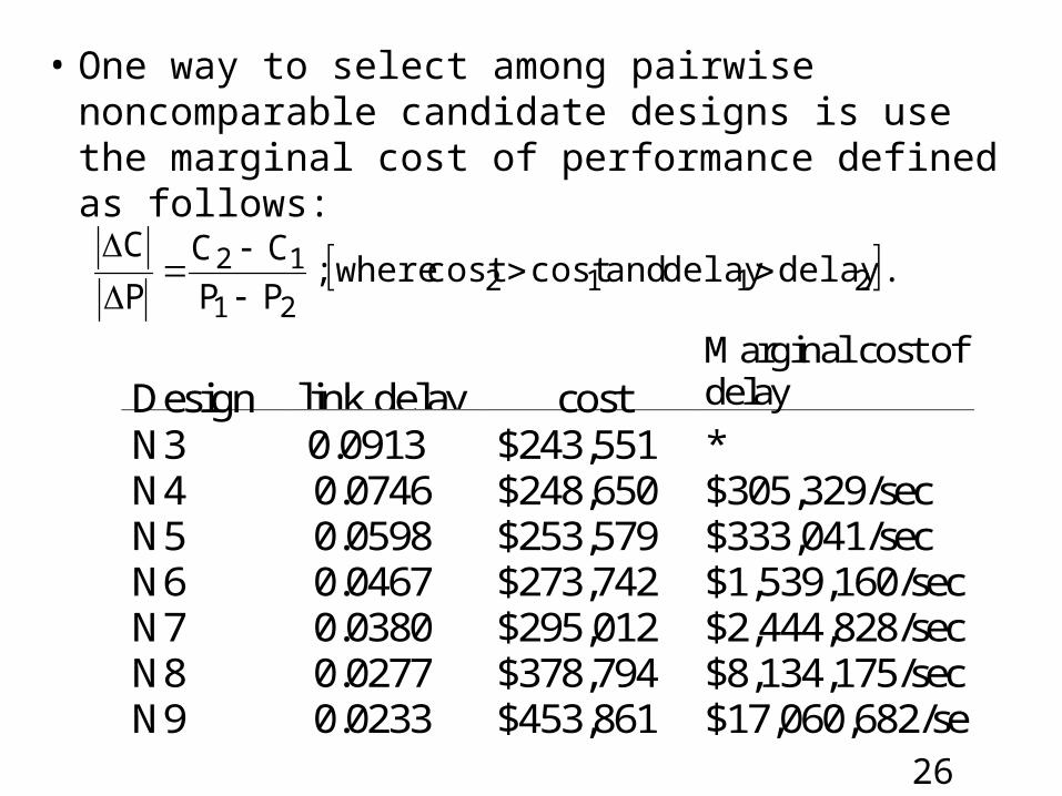
• One way to select among pairwise noncomparable candidate designs is use the marginal cost of performance defined as follows:

.delaydelay andcostcost where;PP

CC

P

C2112

21

12

Design link delay costMarginal cost ofdelay

N3N4N5N6N7N8N9

0.09130.07460.05980.04670.03800.02770.0233

$243,551$248,650$253,579$273,742$295,012$378,794$453,861

*$305,329/sec$333,041/sec$1,539,160/sec$2,444,828/sec$8,134,175/sec$17,060,682/se