1

TCOM 501: Networking Theory & Fundamentals

Lecture 8

March 19, 2003

Prof. Yannis A. Korilis

8-2 Topics

Closed Jackson Networks Convolution Algorithm Calculating the Throughput in a Closed Network Arrival Theorem for Closed Networks Mean-Value Analysis Norton’s Equivalent

8-3 Closed Jackson Networks

Closed Network: K nodes with exponential servers No external arrivals (γi=0) , no departures (ri0=0) Fixed number M of circulating customers

Appropriate model for systems with “limited” resources, e.g., flow control mechanisms

Steady-state distribution will be shown to be of “product-form” type

1

2

3

4

5

1

2

43

551r

53r

M

8-4 Closed Jackson Network

Aggregate arrival rates

Relative arrival rates – visit ratios Can only be determined up to a constant Use an additional equation to obtain unique solution to the above system, e.g.

Set λj=1, for some node j

Set λj=μj, for some node j

Set λ1+ λ2+…+ λK=1

ni: number of customers at node i

Possible states for the closed network n=(n1, n2,…,nK), with

Let F(M) denote the set of all such states

1

2

3

4

5

1 2

43

551r

53r

M

1, 1,...,

K

i j jijr i K

10 and | |

K

i iin n n M

8-5 Closed Jackson Network

Let xi be the number of customers at station i, at steady state

Random variables x1, x2,…, xK are not independent – their sum must be equal to M

The state x=(x1, x2,…, xK) of the closed network can take values n=(n1, n2,…,nK), with

Let F(M) denote the set of all such states Define ρi ≡ λi/μi – this is not the actual utilization factor of station i Jackson’s theorem for closed networks gives the stationary distribution

10 and | |

K

i iin n n M

1 1( ) { } { , , }K Kp n P x n P x n x n

8-6

Theorem 1: The stationary distribution of a closed Jackson network is

where the normalization constant G(M) is a function of M G(M) guarantees that {p(n)} is a valid probability distribution

This stationary distribution is said to have a product-form However: at steady-state the queues are not independent

{pi(ni)}: marginal stationary distribution of queue i

Jackson’s Theorem for Closed Networks

1

1( ) , for all ( ) { : 0, | | }

( )i

Kn

i ii

p n n M n n n MG M

F

( ) ( ) 1

( ) 1 ( ) i

Kn

in M n M i

p n G M

F F

1 1( ) ( ) ( )K Kp n p n p n

8-7 Jackson’s Theorem for Closed Networks (proof)

Theorem 2: The reversed chain of a stationary closed Jackson network is also a stationary closed Jackson network with the same service rates and routing probabilities:

Proof of Theorems 1 & 2: Show that for the corresponding forward and reversed chains

Need to prove only for m=Tijn

Verify, exactly as in the open-network case, that:

* /ij j ji ir r

*( ) ( , ) ( ) ( , ), , ( ),p m q m n p n q n m n m M n m F

* * *( , ) ( , ) { 1 0} ( / )ij i j j ji i j i ij jq T n n q n e e n r n r 1*

1

( ) ( , ) ( ) ( , ) ( ) ( / ) ( ) 1{ 0}

( ) ( )1{ 0}ij ij ij ij j i ij j i ij i

ij j i i

p T n q T n n p n q n T n p T n r p n r n

p T n p n n

( , ) { 0}ij i ij iq n T n r n 1

*( , ) ( , ) 1{ 0}, ( )i im n m n i

q n m q n m n n M

F

8-8 Closed Jackson Network

Example: Closed network model for CPU (rate μ1) and I/O (rate μ2) system. Upon service completion in 1, customer routed to 2 with probability p2=1-p1, or back to 1 with probability p1. M =fixed number of customers

Stationary distribution: n customers in 2 and M-n in 1

Normalization constant

Utilization factor and throughput of node 1:

1

2

1p

2p

2

1

1 1 1 2 2 2 1 1 1 2 2 1, . Choose solution: and p p p 2 1

1 22

1, p

1 2 2

1 1( , ) , 0,1,...,

( ) ( )M n n np M n n n M

G M G M

12

202

1( )

1

MM nn

G M

2 ( 1)( ) 1 (0, ) 1

( ) ( )

M G MU M p M

G M G M

1 1 1

( 1)( ) ( )

( )

G MM U M

G M

8-9 Closed Networks: Normalization Constant

Normalization constant as a function of M and K:

All performance measures of interest – throughput, average delay – can be obtained in terms of G(M,K)

Computational complexity is exponential in M and K:

Recursive methods can be used to reduce complexity Iterative algorithm [due to Buzen]

Normalization constant will be treated as a function of both M and K and denoted G(M,K) only in the context of the iterative algorithm

1 2

1

1 2( ) 1

0

( , ) i K

K

i

Kn n n n

i Kn M i n n M

n

G M K

F

1 terms in the summation

M K

M

8-10 Iterative Computation of G(M)

For any m and k (m=0,…, M; k=1,…, K) define:

For a closed network of single-server queues G(M,K) can be computed iteratively using the following recursive relation:

with boundary conditions:

1 2

1

1 2( ) 1

( , ) i k

k

kn nn n

i kn m i n n m

G m k

F

( , ) ( , 1) ( 1, )kG m k G m k G m k

1( ,1) , 0,1,...,

(0, ) 1, 1,2,...,

mG m m M

G k k K

8-11 Iterative Algorithm (proof)For 0 and 1m k we split the sum into two sums over disjoint sets of states, corresponding to 0,kn and 0kn .

1 2

1

1 2 1 2

1 1

11 2 1 2

1 1 1

1 2

1 2 1 2

0 0

1 2 1 1 2

0

( , ) k

k

k k

k k

k k

k k

k k

k

nn nk

n n M

n nn n n nk k

n n m n n mn n

n nn n n nk k

n n m n n mn

G m k

Note that the first sum is ( , 1).G m k For the second sum, observing that 0,kn we define

1,k kn n where 0.kn Then:

1 2 1 2

1 1

1 2

1

11 2 1 2

10 0

1 21

0

( 1, )

k k

k k

k k

k

k

k

n nn n n nk k

n n m n n mn n

nn nk k k

n n mn

G m k

Therefore: ( , ) ( , 1) ( 1, )kG m k G m k G m k

8-12 Iterative Algorithm – Example

43

551

1

2r

53

1

2r

M

2 22

1

Visit ratios λi determined up to a multiplicative constant

Letting λ1= 2μ, we have: Calculation of G(M,5) based on the iterative algorithm using these values

1 2 3 4

51 53 1 3

5 1 3 1

,

2

r r

1 2 1 3 4 3 1

5 5 1 1

/ 2 , / 2

/ 2 / 4 / , with /

1 2 3 4 51, 2, 4 /

8-13 Iterative Algorithm – Example

Boundary conditions:

Iteration:

1 2 3 4 5

0 1 1 1 1 1 1 1 2 4 6 6+4/ρ 2 1 3 11 23 23+(6+4/ρ)(4/ρ) 3 1 4 26 72 72+[23+(6+4/ρ)(4/ρ)](4/ρ)

km

1 2 3 4 51, 2, 4 /

1( ,1) , 0,1,...,

(0, ) 1, 1,2,...,

mG m m M

G k k K

( , ) ( , 1) ( 1, )kG m k G m k G m k

Example:

2

3

2

(1,2) (1,1) (0,2) 1 1 2

(1,3) (1,2) (0,3) 2 2 4

(2,2) (2,1) (1,2) 1 2 3

G G G

G G G

G G G

8-14 Marginal Distribution

Proposition 1: In a closed Jackson network with M customers, the probability that at steady-state, the number of customers in station j greater than or equal to m is:

Proof 1:

( ){ } , 0

( )m

j j

G M mP x m m M

G M

1

1

1

1

1

1

1

( )

1

1

0

{ } ( )( )

( )

( )

( )( )

j K

j K

j j

j K

j K

j

j K

j K

j

nn nj K

jn M n n n M

n m n m

n mn nj K

n n m n Mn m m

mnj n nj K

n n n M mn

mj

P x m p nG M

G M

G M

G M mG M

F

8-15 Marginal Distribution

Proposition 2: In a closed Jackson network with M customers, the probability that in steady state there are m customers at station j is:

Proof 2:

Proposition 3: In a closed Jackson network with M customers, the average number of customers at queue j is:

Proof 3:

( ) ( 1){ } , 0

( )m i

j j

G M m G M mP x m m M

G M

{ } { } { 1}j j jP x m P x m P x m

1 1

( )[ ] { }

( )

M Mm

j j j jm m

G M mN E x P x m

G M

1

( )( )

( )

Mm

j jm

G M mN M

G M

8-16

Proposition 4: In a closed Jackson network with M customers, the average throughput of queue j is:

Proof 4: Average throughput is the average rate at which customers are serviced in the queue. For a single-server queue the service rate is μj when there are one or more customers in the queue, and 0 when the queue is empty. Thus:

Average Throughput

( 1)( )

( )j j

G MM

G M

( 1) ( 1)( ) { 1}

( ) ( )j j j j j j

G M G MM P x

G M G M

8-17 Example: ./M/1 Queues in Tandem

1 2 K

Choose 1 2 1, 1,...,K i i K

1 21 2

( ) ( )

1 ( 1)!( ) 1

!( 1)!Kn n n

Kn M n M

M K M KG M

M M K

F F

1

1 1 !( 1)!( ) , for all ( )

1( ) ( 1)!i

Kn

ii

M Kp n n M

M KG M M K

M

F

M

K21

( )M

8-18 Example: ./M/1 Queues in Tandem (cont.)

Average throughput:

For queue j=1,…,K:

Average time-delay:

M

K21

( )M

( 1) ( 2)! !( 1)!( ) ( )

( ) ( 1)!( 1)! ( 1)!

1

j j

G M M K M KM M

G M M K M K

M

M K

( )

( ) 1 1 1 1( )

( )

j

jj

j

MN M

KN M M M K M K

T MM K M K

1( ) ( )jj

M KT M T M

8-19 Arrival Theorem for Closed Networks

Theorem: In a closed Jackson network with M customers, the occupancy distribution seen by a customer upon arrival at queue j is the same as the occupancy distribution in a closed network with the arriving customer removed.

Corollary: In a closed network with M customers, the expected number of customers found upon arrival by a customer at queue j is equal to the average number of customers at queue j, when the total number of customers in the closed network is M-1.

Intuition: an arriving customer sees the system at a state that does not include itself.

8-20 Arrival Theorem (proof) 1( ) ( ( ),..., ( ))Kx t x t x t state of the network at time t

( )ijT t probability that a customer moves from station i to j, at time t+

For any state ( )n MF with 0in , find the conditional probability that a customer

moving from node i to node j finds the network at state n

1

1

( )0

1

1( ) ( )0 0

{ ( ) , ( )} { ( ) } { ( ) | ( ) }( ) { ( ) | ( )}

{ ( )} { ( ) } { ( ) | ( ) }

( )

( )

i

i K

i K

i i

ij ijij ij

ij ijm M

m

nn ni ij i K

mm mi ij i K

m M m Mm m

P x t n T t P x t n P T t x t nn P x t n T t

P T t P x t m P T t x t m

p n r

p m r

F

F F

Changing index 1, 0i i im m m in the sum in the denominator:

1

1

1

1 1

1

1

11

111 0

1 11 1

11

0

( )

( 1)

i K

i K

i K

i

i iK K

i K

i K

i

nn ni K

ij mm mi K

m m m Mm

n nn n n ni K i K

mm mi K

m m m Mm

n

G M

This is the probability of state 1( , , 1, )i Kn n n in an identical network with M-1

customers

8-21 Mean-Value Analysis Closed network with M customers; performance measures

Nj(M): average number of customers in queue j

Tj(M): average a customer spends (per visit) in queue j

γj(M): average throughput of queue j

Mean-Value Analysis: Calculates Nj(M) and Tj(M) directly, without first computing G(M) or deriving the stationary distribution of the network

Iterative calculation:

with initial condition:

Average throughput

1

1 ( 1)( ) , 1,..., ; 1,...,

( )( ) , 1,..., ; 1,...,

( )

jj

j

j jj K

i ii

N mT m j K m M

T mN m m j K m M

T m

(0) 0, 1,...,jN j K

( )( ) , 1,..., ; 1,...,

( )j

jj

N mm j K m M

T m

8-22

Arrival Theorem → expected number of customers that an arrival finds at queue j is Nj(m-1). Service rate for all customer at the queue μj.

λ1,…,λK: visit ratios – a solution to flow conservation equations Actual throughput of queue j: Using Little’s Theorem:

Summing for all j and noting that ∑j Nj(m) = m:

Then:

Mean Value Analysis (proof)

1 ( 1)( ) , 1,..., ; 1,...,j

jj

N mT m j K m M

( ) ( 1) / ( ) ( )j j jm G m G m m

( ) ( ) ( ) ( ) ( )j j j j jN m m T m m T m

1 11

( ) ( ) ( ) ( )( )

K K

i i i Ki i i ii

mm N m m T m m

T m

1

( )( ) , 1,..., ; 1,...,

( )j j

j K

i ii

T mN m m j K m M

T m

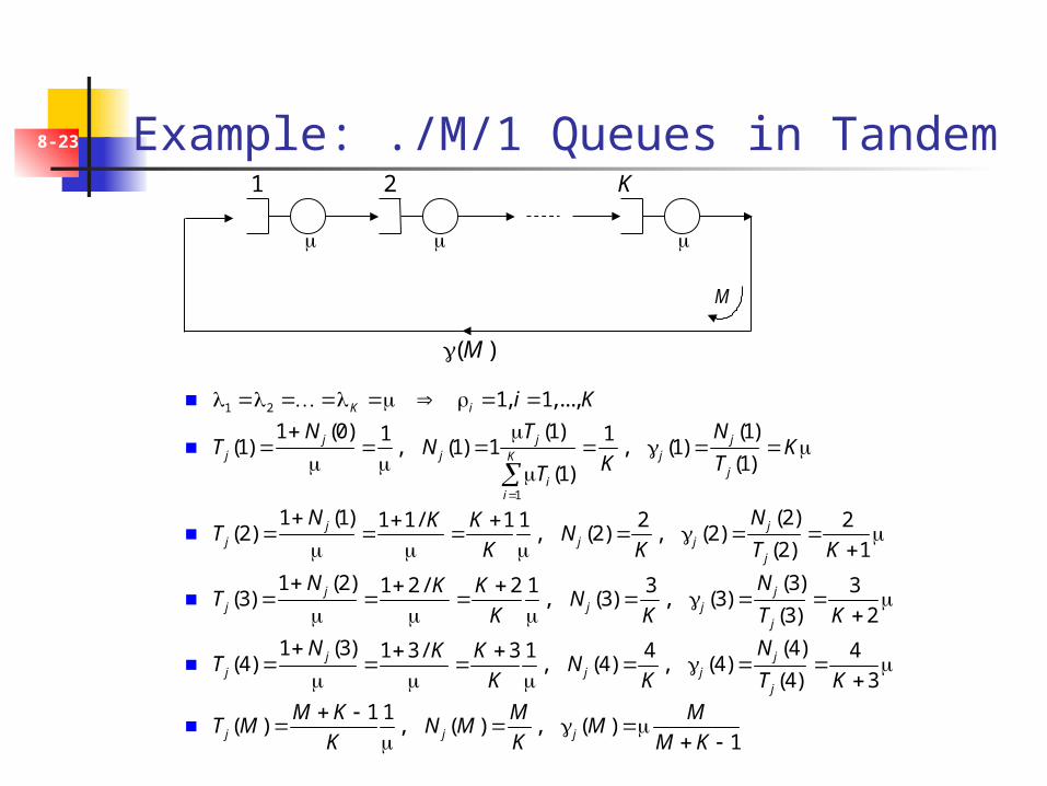
8-23 Example: ./M/1 Queues in Tandem

M

K21

( )M

1 2 1, 1,...,K i i K

1

1 (0) (1) (1)1 1(1) , (1) 1 , (1)

(1)(1)

j j jj j jK

ji

i

N T NT N K

K TT

1 (1) (2)1 1/ 1 1 2 2

(2) , (2) , (2)(2) 1

j jj j j

j

N NK KT N

K K T K

1 (2) (3)1 2 / 2 1 3 3

(3) , (3) , (3)(3) 2

j jj j j

j

N NK KT N

K K T K

1 (3) (4)1 3/ 3 1 4 4

(4) , (4) , (4)(4) 3

j jj j j

j

N NK KT N

K K T K

1 1

( ) , ( ) , ( )1j j j

M K M MT M N M M

K K M K

8-24 State-Dependent Service Rates

Theorem: The stationary distribution of a closed Jackson network where the nodes have state-dependent service rates is

where the normalization constant G(M) is a function of M, the fixed number of customers in the network

Normalization constant:

Proof similar to the one for open networks

1

1( ) , for all ( ) { : 0, | | }

( ) (1) ( )

inKi

ii i i i

p n n K n n n KG M n

F

( ) 1 ( )

( ) ( ) 1 (1) ( )

inKi

n K i n Ki i i

G M p nn

F F