1

String Lessonsfor

Higher SpinsMassimo TaronnaScuola Normale Superiore & INFN, Pisa

Based on:Master Thesis(2009)[hep-th/1005.3061](M.T. advisor: Prof. A.

Sagnotti)&

hep-th/1006.5242: A.Sagnotti and M.T.

2

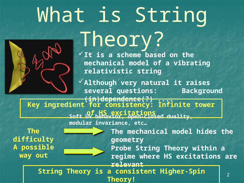
What is String Theory?

It is a scheme based on the mechanical model of a vibrating relativistic string

Although very natural it raises several questions: Background (in)dependence(?) ....

Key ingredient for consistency: Infinite tower of HS excitations

The mechanical model hides the geometry

A possible way out

Probe String Theory within a regime where HS excitations are relevant

The difficulty

Soft UV behavior, open-closed duality, modular invariance, etc…

String Theory is a consistent Higher-Spin Theory!

3

Higher Spins and Field Theory

Starting Point Symmetry group of space-time

(Majorana, 1932; Dirac, 1936; Fierz-Pauli, 1939; Wigner, 1939; …)

Fundamental one-particle states are labeled by two quantum numbers

Mass:

m2 ¸ 0 Spin:

s = 0;12

; 1;32

; 2;52

; 3; : : :More labels

forD ¸ 5

There is at present no indication about the existence of a preferred subset of values!

The Challenge

Uncover the systematics of Higher Spins

4

Constructing a non-linear Gauge Theory

Postulate some non-abelian algebra and construct the corresponding invariant field theoryAnalyze vertices in a preexisting non linear theory

Classify all consistent deformations of the free theory (Nöther procedure)

Low spin High spin

YANG-MILLS

GENERAL RELATIVITY

SUGRA

VASILIEV’s SYSTEM

STRING (FIELD) THEORY

Bengtsson,; Ouvry and Stern (1986)

. . .M.T. (2009)

A. Sagnotti and M.T. (2010)

Berends, Burgers, van Dam(1985)

Barnich, Hanneaux (1993). . .

Bekaert (2008)Bekaert , Joung, Mourad

(2009)Manvelyan, Mktrchyan, Rühl

(2010)Fotopoulos, Tsulaia (2010)

5

Conjectures and Open problems

Does string theory result from the spontaneous breaking of HS gauge symmetry?

How unique is String Theory?

Using String Theory as a theoretical laboratory one can extract a lot of information about consistent

interactions of HS statesMassive scattering amplitudes and couplings do

not suffer from the usual problems encountered in the massless case

In the massless limit ordinary gauge invariance emerges!

D. Gross; E.S. Fradkin; …

6

Plan Open Bosonic String Tree-level S-matrix

Amplitudes String symbol calculus Generating function for 3-point correlation functions 3-point Amplitudes

String Higher-Spin Couplings Couplings 0-0-s Couplings 1-1-s General case Higher-Spin Conserved Currents

7

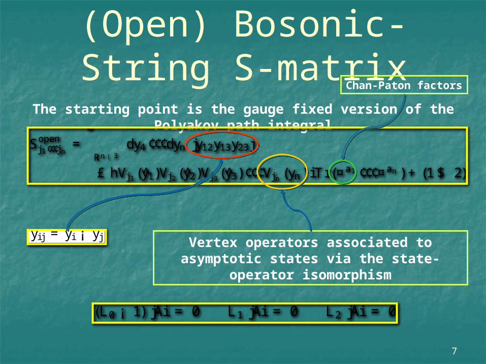
(Open) Bosonic-String S-matrix

The starting point is the gauge fixed version of the Polyakov path integral

Vertex operators associated to asymptotic states via the state-

operator isomorphism

Sopenj 1¢¢¢j n

=Z

Rn ¡ 3dy4 ¢¢¢dyn jy12y13y23j

£ hVj 1(y1)Vj 2(y2)Vj 3(y3) ¢¢¢Vj n (yn) iTr(¤a1 ¢¢¢¤an ) + (1$ 2)

yi j = yi ¡ yj

Chan-Paton factors

(L0 ¡ 1) jÁi = 0 L1 jÁi = 0 L2 jÁi = 0

8

Symbol CalculusIt is convenient to introduce the symbols of

the usual string oscillators

In terms of symbols the usual vertex operator correlation function that enters into the definition of the S-matrix

becomes

hÁ1(y1; p1) :: : Án(yn; pn) i = [Á1(»1) :: : Án(»n)] ? Z(»i )

Symbol of the vertex operator

? : Á(»1);Ã(»2) ! Á?Ã = expµ

@@»1

¢@

@»2

¶Á(»1)Ã(»2)

¯¯¯» i = 0

= Á(0) Ã (0) +Á(1) ¹ Ã (1)¹ +

12

Á(2) ¹ 1¹ 2 Ã ;(2)¹ 1¹ 2

+:::

Weyl-Wigner calculus!

Generating Function

Ái (pi ;»i ) =X

n

1n!

Ái ¹ 1¢¢¢¹ n »¹ 1i : : : »¹ n

i = Á(0)i +»¹

i Á(1)i ¹ +»¹ 1

i »¹ 2i Á(2)

¹ 1¹ 2+:::

9

Z = i(2¼)d±(d)(J 0) Cexp

2

4¡12

nX

i6=j

®0pi ¢pj lnjyi j j ¡p

2a0 »i ¢pj

yi j+

12

»i ¢»j

y2i j

3

5

Generating Functions

For external states of the first Regge trajectory of the open bosonic string

Ái (pi ;»i ) =1X

n = 0

1n!

Ái ¹ 1¢¢¢¹ n »¹ 1i : : : »¹ n

i

Unphysical dependence on the yij

10

Three-point Amplitudes

¡ p21 =

s1 ¡ 1®0 ¡ p2

2 =s2 ¡ 1

®0 ¡ p23 =

s3 ¡ 1®0

Zphys = igo(2¼)d

®0 ±(d)(p1+p2+p3) exp

( r®0

2

µ»1 ¢p23

¿y23

y12y13

À+ »2 ¢p31

¿y13

y12y23

À+ »3 ¢p12

¿y12

y13y23

À¶+ (»1 ¢»2 + »1 ¢»3 + »2 ¢»3)

)

L0 constraint: mass parameterization for the

first Regge trajectory

The issue is now to impose the Virasoro

constraints at the level of the generating

function in order to select the physical information that it

containsL1 constraint: transversality

One thus obtains the physical generating function for three-point amplitudes

hxi = sign(x)

L2 constraint: tracelessness

[Á1(»1) Á2(»2) Á3(»3)] ? Zphys

11

Three-point AmplitudesThe amplitudes are given by the

* - product of the physical

generating function with the symbols of the vertex operators

Ái (pi ; »i ) =1X

n=0

1n!

Ái ¹ 1¢¢¢¹ n »¹ 1i : : : »¹ n

i The result is

A = igo

®0 (2¼)d±(d)(p1 + p2 + p3) fA +(p1;p2;p3)Tr [¤a1 ¤a2¤a3 ]+ A ¡ (p1;p2;p3)Tr [¤a2 ¤a1¤a3 ]g

A § = Á1

Ã

p1;@@»

§

r®0

2p31

!

Á2

Ã

p2; » +@@»

§

r®0

2p23

!

Á3

Ã

p3; » §

r®0

2p12

! ¯¯¯¯¯»= 0

Carrying out the * - product one

arrives at

Analogous simplifications for four-point amplitudes and string currents!

12

0-0-s CouplingsIn this case the current generating function is conserved and is given by

J = igo

®0 f J +(x;») Tr[ ¢¤a1 ¤a2 ] + J ¡ (x;») Tr[ ¢¤a2 ¤a1 ]g

J § (x;») = ©

Ã

x § i

r®0

2»

!

©

Ã

x ¨ i

r®0

2»

!coordinate space

(Berends, Burgers and Van Dam, 1986)

(Bekaert, Joung, Mourad, 2009)

= Á(x)¤Á(x) + i

r®0

2»¹

hÁ¤(x)@¹ Á(x) ¡ Á(x)@¹ Á¤(x)

i+ :: :

Example: the complex scalar

HS currents

13

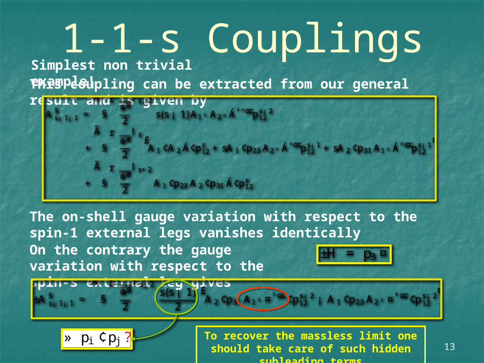
1-1-s CouplingsThis coupling can be extracted from our general result and is given by

A §s¡ 1¡ 1 =

Ã

§

r®0

2

! s¡ 2

s(s ¡ 1) A1¹ A2º Á¹ º ¢¢¢ps¡ 212

+

Ã

§

r®0

2

! s£A 1 ¢A 2 Á¢ps

12 + sA 1 ¢p23 A2º Áº ¢¢¢ps¡ 112 + sA 2 ¢p31 A1º Áº ¢¢¢ps¡ 1

12

¤

+

Ã

§

r®0

2

! s+2

A 1 ¢p23 A 2 ¢p31 Á¢ps12

The on-shell gauge variation with respect to the spin-1 external legs vanishes identicallyOn the contrary the gauge variation with respect to the spin-s external leg gives

±H = p3 ¤

±A §s¡ 1¡ 1 =

Ã

§

r®0

2

! s¡ 2s(s ¡ 1)

2

£A 2 ¢p31 A1¹ ¤¹ ¢¢¢¢ps¡ 2

12 ¡ A 1 ¢p23 A2¹ ¤¹ ¢¢¢¢ps¡ 212

¤

» pi ¢pj ? To recover the massless limit one should take care of such hidden

subleading terms

Simplest non trivial example!

14

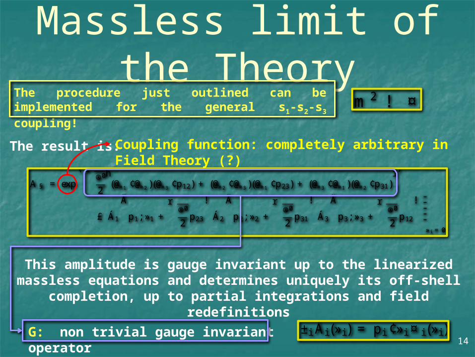
Massless limit of the Theory

The procedure just outlined can be implemented for the general s1-s2-s3 coupling!

This amplitude is gauge invariant up to the linearized massless equations and determines uniquely its off-shell

completion, up to partial integrations and field redefinitions

m2 ! ¤

The result is:

A § = exp

( r®0

2

h(@»1 ¢@»2 )(@»3 ¢p12) + (@»2 ¢@»3 )(@»1 ¢p23) + (@»3 ¢@»1 )(@»2 ¢p31)

i)

£ Á1

Ã

p1; »1 +

r®0

2p23

!

Á2

Ã

p2; »2 +

r®0

2p31

!

Á3

Ã

p3; »3 +

r®0

2p12

! ¯¯¯¯¯» i = 0

G: non trivial gauge invariant operator

±i Ái (»i ) = pi ¢»i ¤ i (»i )

Coupling function: completely arbitrary in Field Theory (?)

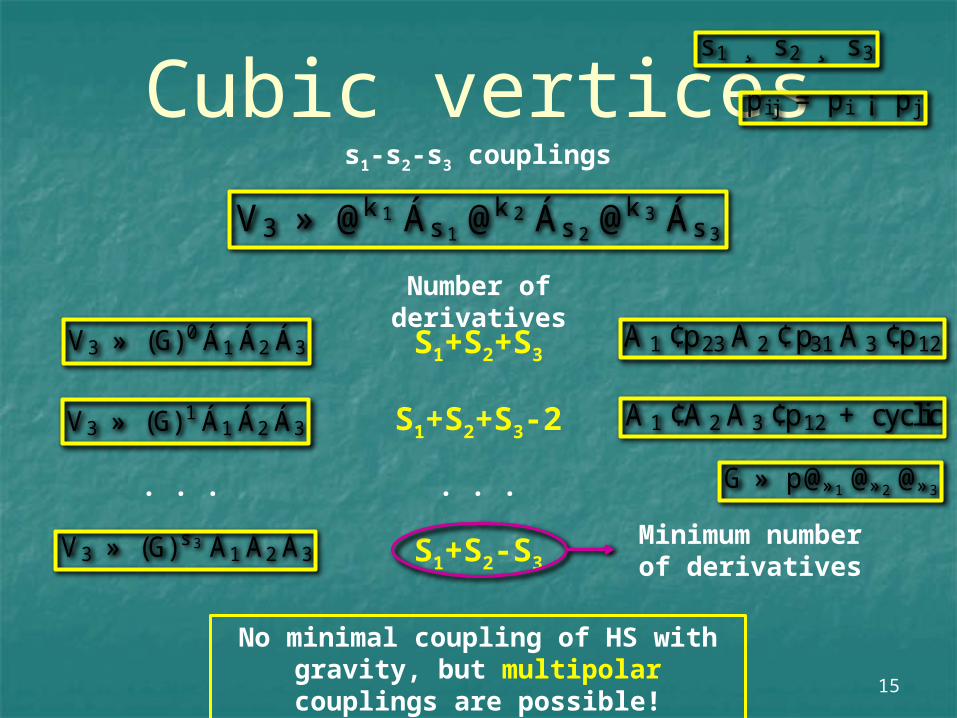
15

Cubic verticesV3 » @k 1 Ás 1 @k 2 Ás 2 @k 3 Ás 3

s1-s2-s3 couplings

V3 » (G) 0 Á1 Á2 Á3

Number of derivativesS1+S2+S3

s1 ¸ s2 ¸ s3

V3 » (G) 1 Á1 Á2 Á3 S1+S2+S3-2 A 1 ¢A 2 A 3 ¢p12 + cyclic

A 1 ¢p23 A 2 ¢p31 A 3 ¢p12

pi j = pi ¡ pj

V3 » (G) s 3 Á1 Á2 Á3 S1+S2-S3

. . . . . .

Minimum number of derivatives

No minimal coupling of HS with gravity, but multipolar couplings

are possible!

G » p@»1 @»2 @»3

16

HS (bosonic) Conserved CurrentsThe couplings so far obtained are induced by

Noether currents

J § (x ; ») = exp

Ã

¨ i

r®0

2»®

£@³1 ¢@³2 @®

12 ¡ 2@®³1

@³2 ¢@1 + 2@®³2

@³1 ¢@2¤!

£ Á1

Ã

x ¨ i

r®0

2»; ³1 ¨ i

p2®0@2

!

Á2

Ã

x § i

r®0

2»; ³2 § i

p2®0@1

! ¯¯¯¯¯³ i = 0

Conserved up to massless Klein-Gordon equation, divergences and traces, but their completion turns out

to be completely fixed, up to redefinitions!

J (x ; ») = J (0)(x) + »¹ J (1)¹ (x) + :::

Spin one currents

HS currents

17

HS (fermionic) Conserved CurrentsAn educated guess is possible in the

fermionic case

J [0]§F F (x ; ») = exp

Ã

¨ i

r®0

2»®

£@³1 ¢@³2 @®

12 ¡ 2@®³1

@³2 ¢@1 + 2@®³2

@³1 ¢@2¤!

£ ¹ª 1

Ã

x ¨ i

r®0

2»; ³1 ¨ i

p2®0@2

!h1 + =»

iª 2

Ã

x § i

r®0

2»; ³2 § i

p2®0@1

! ¯¯¯¯¯³ i = 0

Conserved up to massless Dirac equation, divergences and (gamma-)traces, but their completion turns out to

be completely fixed, up to redefinitions!

J (x ; ») = J 0(x) + »¹ ( ¹Ã ° ¹ à + :::) + :: :

Spin one currents

HS currents

Analogous result for the currents with one fermion and one boson

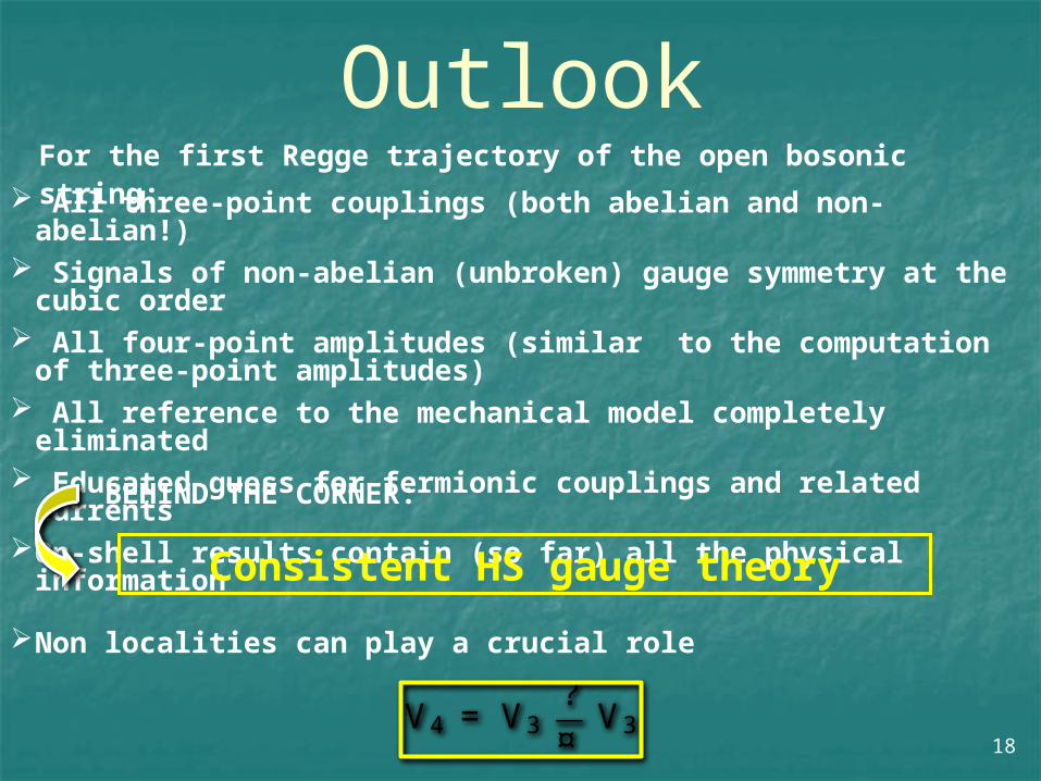
Outlook All three-point couplings (both abelian and non-abelian!) Signals of non-abelian (unbroken) gauge symmetry at the

cubic order All four-point amplitudes (similar to the computation of

three-point amplitudes) All reference to the mechanical model completely

eliminated Educated guess for fermionic couplings and related

currentsOn-shell results contain (so far) all the physical information

For the first Regge trajectory of the open bosonic string:

BEHIND THE CORNER:

Consistent HS gauge theory

Non localities can play a crucial role

18V4 = V3

?¤

V3