1

Space-Efficient Tracking of Persistent

Items in a Massive Data StreamBibudh Lahiri and Srikanta Tirthapura and Jaideep Chandrashekar

Abstract

Motivated by scenarios in network anomaly detection, we consider the problem of

detecting persistent items in a data stream, which are items that occur “regularly” in

the stream. In contrast with heavy-hitters, persistent items do not necessarily contribute

significantly to the volume of a stream, and may escape detection by traditional volume-

based anomaly detectors.

We first show that any online algorithm that tracks persistent items exactly must

necessarily use a large workspace, and is infeasible to run on a traffic monitoring node. In

light of this lower bound, we introduce an approximate formulation of the problem and present

a small-space algorithm to approximately track persistent items over a large data stream. We

experimented with three different datasets to see how the accuracy and memory footprint

of the algorithm varies with the skewness of the dataset. Our algorithms performed best for

the two datasets out of three which had highest skewness of persistence and lowest mean

persistence. To our knowledge, this is the first systematic study of the problem of detecting

persistent items in a data stream, and our work can help detect anomalies that are temporal,

rather than volume based.

Index Terms

Data streams; persistence; sketches; hash-based filters

F

• The work of Bibudh Lahiri and Srikanta Tirthapura was supported in part by grants 0834743 and 0831903 from theNational Science Foundation.E-mail: bibudhlahiri@gmail.com, jaideepcs@gmail.com, snt@iastate.edu

• Bibudh Lahiri is with Impetus Technologies, Los Gatos, CA. Srikanta Tirthapura is with the Department of Electricaland Computer Engineering, Iowa State University, Ames, IA. Jaideep Chandrashekar is with Technicolor Labs, Paris.

A preliminary version of this paper appeared in the Proceedings of the 5th ACM International Conference on DistributedEvent-Based System, 2011

2

1 INTRODUCTION

We consider the problem of tracking persistent items in a large data stream. This problem

has particular relevance while mining various network streams, such as the traffic at a

gateway router, connections to a web service, etc. Informally, a persistent item is one that

occurs “regularly” in the stream.

More precisely, suppose that the time at the stream processor is partitioned into non-

overlapping intervals called “timeslots”. Consider a stream of elements of the form (d, t)

where d is an item identifier, and t is a timeslot during which the item arrived. The t

values are in an increasing order within the stream. Multiple items can arrive in the same

timeslot, and the same item may arrive multiple times within a time slot. Suppose the

total number of timeslots in the stream is n. The persistence of an item d is defined to be

the number of distinct timeslots in which d was observed. The persistence of any item

is an integer between 0 and n (inclusive). An item is said to be α-persistent, for some

constant 0 < α ≤ 1, if its persistence is at least αn. Given a user-defined α, the problem

is to output the set of α-persistent items in the stream.

Persistent items exhibit a repeated and regular pattern of arrival, and are significant

for many applications. Giroire et al. [1] monitored traffic from end-hosts to detect com-

munication across botnet channels. They observed that persistent destinations were likely

to belong to one of two classes: (1) either they were malicious hosts associated with a

botnet, or (2) they were frequently visited benign hosts. It was also observed that the latter

set of hosts could be identified easily and assembled into a “whitelist” of known good

destinations. They found that tracking persistent items in the network stream, followed

by filtering out items contained in the whitelist, resulted in reliable identification of botnet

traffic.

More broadly, persistent items are often associated with specific anomalies in the con-

text of network streams: periodic connections to an online advertisement in a pay-per-

click revenue model [2] is an indicator of click fraud [3], repeated (failed) connections

observed in the stream is indicative of a failed or unreachable web service [4]; botnets

periodically “phone home” to their bot controllers [1]; attackers regularly scan for open

3

ports on which vulnerable applications are usually deployed [5]. While the narrative in

this paper draws from applications in the network monitoring space, it appears that the

problem of detecting persistent items in a data stream is broadly applicable in other

data monitoring applications. For example, persistent use of gathering techniques such

as telephone interception or satellite imaging might indicate an “Advanced Persistent

Threat” (APT) [6] for a target group, e.g., a government.

The persistent items in a stream could be very different from the frequently occurring

items (or “heavy-hitters”) in a stream. An item is called a φ-heavy hitter if it contributes to

at least a φ fraction of the entire volume of the stream. There is a large body of literature

on heavy-hitter identification (including [7], [8], [9], [10], [11], [12]). A persistent item

need not be a heavy hitter. For example, the item may appear only once in each time slot

and may not contribute significantly to the stream volume. Such “stealthy” behavior was

indeed observed in botnet traffic detection [1]; the highly persistent destinations which

were not contained in the whitelist did not contribute in any meaningful way to the

traffic volume. In fact, the traffic to these destinations was stealthy and very low volume,

perhaps by design to evade detection by traditional volume-based detectors. Conversely,

a heavy-hitter need not be a persistent item either – for example, an item may occur

a number of times in the stream, but all its occurrences maybe within only a couple of

timeslots. Such an item will have a low persistence. Clearly, the set of persistent items in a

stream can be very different from the set of heavy-hitters in the stream; their intersection

can very well be empty. There seems to be no easy reduction from the problem of tracking

persistent items to the problem of tracking heavy-hitters. For example, one could attempt

to devise a “filter” that eliminated duplicate occurrences of an item within a time slot,

and then apply a traditional heavy-hitter algorithm on the resulting “filtered” stream. But

this approach does not work in small space, because such a filter would itself take space

proportional to the number of distinct items that appeared within the timeslot, and this

number maybe very large, especially for the type of network traffic streams that we are

interested in.

A closely related problem is the problem of identifying heavy distinct hitters (HDHs)

4

in a data stream (Venkataraman et al.[13] and Bandi et. al. [14]). In the heavy distinct

hitters problem, we are given a stream S′ of (x, y) pairs, of length N . For a parameter

β, 0 < β ≤ 1, the set of β-HDHs in S′ is defined as the set of all those values of x that

have occurred with more than Nβ distinct values of y. There is a reduction from the

problem of tracking persistent items to that of identifying HDHs, as follows. Consider

the identification of α-persistent items on a stream S of (d, t) pairs, of length N . Let n

denote the total number of timeslots in S. Consider a stream S′ of (x, y) pairs where for

each element (d, t) ∈ S, there is an element (x = d, y = t) in S′. Then, the nαN -HDHs in

S′ are the set of α-persistent items in S. There are two significant issues with using such

a reduction for solving our problem using an algorithm (such as in [13], [14]) for HDH

identification. (1)The first one is that for HDH identification, the threshold nαN should be

known beforehand. Though n, the number of timeslots is usually known before the stream

is observed, the number of packets N is not known beforehand, so the prior algorithms

for HDHs cannot be directly used. (2)Next, even if we were to modify the algorithms for

HDHs to work with an “adaptive threshold”, that can change as the number of elements

increases (which seems non-trivial), there is special structure in the data in the persistent

items identification problem that can be used here. In the heavy distinct hitter problem

on a stream of (x, y) values, there is no relative ordering required on the y values, and the

same (x, y) tuple can re-occur at arbitrary positions in the stream. But in the persistent

items problem on a stream of (d, t) tuples, the t values must be in a non-decreasing order

(since they represent the times of observation at the stream processor). An important

consequence of this difference is that the algorithms for HDH identification ([13], [14])

need to use “distinct counters” (such as in [15], [16]) to count the number of distinct y

values associated with each value of x. Hence, the space complexity of their algorithms

is the number of counters maintained multiplied by the space taken by an (approximate)

distinct counter. Approximate distinct counting is inherently expensive space-wise, since

it has been shown [17] that maintaining distinct counters with a relative error of ε requires

Ω(1/ε2) space. Our algorithm does not need to use approximate distinct counters, making

it simpler, more efficient, and easier to implement.

5

Prior work in Giroire et al. [1] used the following method to track persistent items in a

stream of network traffic. For each distinct item in the stream, their method maintained

(1)The number of timeslots in which the item has appeared in the stream so far, and

(2)Whether or not the item has appeared in the current timeslot. This allowed them to

exactly compute the number of timeslots that each item has appeared in, and hence exactly

track the set of persistent items. However, the space taken by this scheme is proportional

to the number of distinct items in the stream. The stream could have a very large number

of distinct items (for example, IP sources, or destinations), and the memory overhead may

render this infeasible on a typical network monitor or a router. Thus the challenge is to

track the persistent items in a stream using a small workspace, and minimal processing

per element. Further, all tracking must be done online, and the system does not have the

luxury of making multiple passes through the data.

1.1 Contributions

In this work, we present the first small-space approximation algorithm for tracking per-

sistent items in a data stream, and an evaluation of the algorithm. Our contributions are

as follows.

Space Lower Bound: We first consider the problem of exactly tracking all α-persistent

items in a stream, for some user-defined α ∈ (0, 1]. For this problem, we show that any

algorithm that solves it must use Ω(m log nα) space, where m is the number of distinct

items in the stream, and n is the total number of slots, even when the number of persistent

items is much smaller than m.

Approximate Tracking of Persistent Items: In light of the above lower bound, we

define an approximate version of the problem. We are given two parameters, α - the

threshold for persistence, and ε < α, an approximation (or “uncertainty”) parameter. The

task is to report a set of items with the following properties: every item that is α-persistent

is reported, and no item with persistence less than (α− ε) is reported. We also formulate

this problem for a “sliding window” of the most recently observed items of the stream.

6

Small Space Algorithm: For the above problem of approximate tracking of persistent

items, we present a randomized algorithm that can approximately track the α-persistent

items using space that is typically much smaller than the number of distinct items in the

stream. The expected space complexity of the algorithm is O(Pεn

), where P is the sum of

the persistence values of all items in the stream, and n is the total number of timeslots. The

algorithm has a small probability of a false negative (i.e. an α-persistent item is missed).

This probability can be made arbitrarily small, at the cost of additional space. Note that

any algorithm will need space that is at least as large as the size of the output, i.e., the

number of α-persistent items in the stream. The worst case scenario is when every item

is α-persistent, forcing the algorithm to use space proportional to the number of distinct

items! Fortunately, this situation does not seem to occur in practice and only a fraction

of items are very persistent, and this helps our algorithm considerably. We also prove

that if persistence of different items in a stream follow a power law distribution, then the

space taken by our algorithm is O(1ε

).

Sliding Windows: In most network monitoring applications, the data set of interest is

not the entire traffic stream, but only a window of the recent past. Formally, we define a

window as follows:

Definition 1.1: A window Sr` consists of all stream elements (di, ti) whose timeslots are

in the range [`, r], i.e. Sr` = (di, ti) ∈ S|` ≤ ti ≤ r.

The size of window Sr` is defined as (r − ` + 1), i.e. the number of timeslots it encom-

passes. For instance, Giroire et al [1] used this sliding window model in their work on

botnet traffic detection. Though the size of the data set has decreased when compared

with the fixed window case, maintaining statistics over a sliding window is still a hard

problem, since the data contained within a sliding window is often too large to be stored

completely within the memory of the stream processor. This is a harder problem than

the fixed window, since it has to deal with (old) elements falling off the window. We

present an extension to our fixed window algorithm to handle the sliding window model.

Interestingly, the expected space cost of our sliding window algorithm is within a factor

of two of the space cost of the fixed window algorithm.

7

Experimental Evaluation: We evaluate our algorithm against three datasets: a large,

real-world network traffic trace (which we call HeaderTrace) collected from an Internet

backbone link, as well as two artifically created datasets, which we call Synthetic1 and

Synthetic2 respectively, the latter having a skewness of persistence (17.17) which is three

times that of the former (5.67). In other words, Synthetic1 had a more uniform distribution

of skewness than Synthetic2 or HeaderTrace.

Our algorithm performed best on HeaderTrace and Synthetic2, and a little worse on

Synthetic1. On HeaderTrace, our small-space algorithm uses up to 85% less space than

the naive algorithm and typically incurs a false positive rate of less than 1% and a false

negative rate of less than 4%. We also see that false positive rate never exceeds 3% for

any parameter setting, while the false negative rate stays below 5% for all but the most

aggressive thresholds for persistence. For Synthetic2, which had a skewness about twice

that of HeaderTrace, the maximum False Positive Rate (FPR) was 2.2%, the typical False

Negative Rate (FNR) being about 6%. The skewness of persistence for the Synthetic1

dataset was about 60% of that of HeaderTrace (9.28). Although the maximum FNR for

Synthetic1 is 11.5% (the theoretical maximum FNR is 13%) and the maximum FPR is

15.6%, the typical FNR and FPR are both within 4%. The comparative performance

on the three datasets shows that our algorithm in fact works better for datasets with

high skewness of peristence and low mean persistence, which is very typical of real-life

network traffic.

1.2 Roadmap

The rest of this paper is organized as follows. A precise statement of the problem is

presented in Section 2, followed by a lower bound on the space cost of exactly tracking

the persistent items in a stream. Our algorithms for the fixed and sliding windows models

are presented in Section 3, followed by their analysis and correctness. Experimental results

are described in Section 4. A detailed discussion of related work is presented in Section

5.

8

2 PROBLEM DEFINITION

Consider a world where time is divided into timeslots (or slots) that are numbered 1, 2, . . ..

Let S be a stream of elements of the form S = 〈(d1, t1), (d2, t2), . . .〉. Each element is a tuple

(di, ti), where di is an item identifier (IP address, hostname, etc), and ti is the time slot

during which the element arrived. It is assumed that the tis are in non-decreasing order.

All elements that have the same values of ti are said to be in the same timeslot. Clearly, a

timeslot consists of elements that form a contiguous subsequence of the observed stream.

The duration of a timeslot depends on the application on hand. In the botnet detection

application [1], the duration of a timeslot was chosen to be between 1 hour and 24

hours, primarily because these were suspected to be the possible lengths of time between

successive connections from the (infected) client to malicious destinations, for the botnets

that they considered. Since then, there have been other botnet attacks that work on a

much smaller timescale (see Section 4 for a discussion). In an eventual solution to botnet

attack detection, we may need to consider running the algorithm simultaneously with

different timeslot durations, to monitor multiple types of attacks.

For a given window Sr` , as defined in Definition 1.1, we define the persistence of an

item in that window as follows:

Definition 2.1: The persistence of an item d over a window Sr` , denoted pd(`, r), is

defined as the number of distinct slots in `, `+ 1, . . . , r that d appeared in.

pd(`, r) = |t|((d, t) ∈ S) ∧ (` ≤ t ≤ r)|

Definition 2.2: An item d is said to be α-persistent in window Sr` if pd(`, r) ≥ α(r−`+1).

In other words, d must have occurred in at least an α fraction of all slots within the

window.

We state two versions of the problem, the first version for a fixed window, and the

second version for a sliding window. In practice, the sliding window version is more

useful.

9

2.1 Exact Tracking of Persistent Items

Problem 1: Identifying Persistent Items Over a Fixed Window: Devise a space-efficient

algorithm that takes as input a prespecified window W = Sn1 and a persistence threshold

α, and at the end of observing the stream, returns the set of all items that are α-persistent.

In other words, the algorithm will report every item that is α-persistent in W and will

not report any item that is not α-persistent.

A straightforward algorithm for this problem would track every distinct item in the

stream, and for each distinct item, count the number of slots (from 0 to n−1) during which

the item appeared. For a single item, its persistence can be tracked in a constant number

of bytes (assuming that the item identifier and slot number can be stored in constant

space), by maintaining a counter for the number of timeslots the item has appeared in

so far, in addition to one bit of state for whether or not the item has appeared in the

current timeslot. The total space consumed by the naive algorithm is of the order of the

number of distinct items in the stream. In general, this would be a large number and

the space overhead may make it infeasible for this algorithm to be deployed within a

network router.

Space Lower Bound for Exact Tracking: We now show that any algorithm that solves

Problem 1 exactly must require Ω(m) space in the worst case, where m is the number

of distinct items in the input. Importantly, Ω(m) space is needed even if the number of

persistent items is much smaller than m.

Lemma 2.1: Any algorithm that can exactly solve Problem 1 must use Ω(m log(nα+ 1))

bits of space in the worst case, where m is the number of distinct items in the input.

Proof: Without loss of generality, suppose that the m distinct items that appear in

the stream are labeled 1, 2, 3, . . . ,m. Consider the state of the stream after observing k =

(n − αn) timeslots. For i from 1 to m, let ni denote the number of timeslots among

1, 2, . . . , k during which item i has appeared. Consider the vector u = 〈n1, n2, . . . , nm〉.

Consider the following set V of possible assignments to u, where each component in u

is chosen from the range 0, 1, 2, . . . , αn. The size of V is (1 + nα)m. We show that any

algorithm that solves Problem 1 must be able to distinguish between two distinct vectors

10

in V , and hence must have a different state of its memory for two input streams that

result in different assignments to u.

We use proof by contradiction. Suppose the above was not true, and there were two

input streams A and B which, at the end of k slots, resulted in vectors vA, vB ∈ V

respectively. Suppose vA 6= vB but the states of the algorithm’s memory were the same

after observing the two inputs. Now, vA and vB must differ in at least one coordinate.

Without loss of generality, suppose they differed in coordinate 1, so n1(A) 6= n1(B),

and without loss of generality suppose n1(A) < n1(B). Consider the rest of the stream,

from slot n − nα onwards. Suppose these slots had nα − n1(B) slots in which item 1

occurred. Clearly, appending this stream to stream A results in a stream with n slots

where the persistence of item 1 is n1(A) + (nα − n1(B)) = nα − (n1(B) − n1(A)) < nα,

and appending this same stream to stream B results in a stream with n slots where the

persistence of item 1 is nα. Thus, item 1 must be reported as α-persistent in the latter

case, and not in the former case. But this is not possible, since the algorithm has the same

memory state for both A and B, and sees the same substream henceforth, leading to a

contradiction.

To distinguish between any two vectors in V , the algorithm needs at least log |V | bits

of memory. Since the size of V is (nα+ 1)m, the lower bound is Ω(m log(nα+ 1)) bits.

2.2 Approximate Tracking of Persistent Items

In light of the above lower bound on the space cost of exact tracking of persistent items,

we define a relaxed version of the problem. Here, in addition to the persistence threshold

α, the user provides two additional parameters, ε ∈ [0, 1], an “uncertainty parameter”,

and δ ∈ [0, 1], an error probability.

Problem 2: Approximate Tracking of Persistent Items over a Fixed Window: Given a

fixed window W = Sn1 , persistence threshold α, approximation parameter ε, and error

probability δ, devise a small space algorithm that returns a set of items with the following

properties.

11

A. If an item is persistent, it is reported with high probability. For any item d, if pd(1, n) ≥ αn,

then d is reported as persistent with a probability at least (1− δ).

B. Items that are far from persistent are not reported. If pd(1, n) < (α − ε) · n, then d is not

reported.

Sliding Windows. The sliding window version of the problem requires that we con-

tinuously monitor the window of the n most recent timeslots in the stream.

Problem 3: Approximately identifying Persistent Items over a Sliding Window: The

problem of approximately tracking persistent items over a sliding window is the same

as the above Problem 2, except that the window of interest, W , is the set of the n most

recent timeslots in the stream, and changes continuously with time.

The fixed window version is a special case of the sliding window, where the window is

equal to the entire stream. The space lower bound for fixed window obviously applies to

the sliding window version, hence it is also necessary to consider an approximate version

of the problem for sliding windows, if we are to achieve a small space solution.

3 AN ALGORITHM FOR APPROXIMATE TRACKING OF PERSISTENT ITEMS

We present algorithms for approximate tracking of persistent items in a stream. We first

present the algorithm for tracking persistent items over a fixed window, followed by a

proof of correctness and analysis of complexity. We then present the algorithm for sliding

window.

3.1 Fixed Window

Intuition. The goal is to track the persistence of as few items in the stream as possible,

and hence minimize the workspace used by the algorithm. Ideally, we track (and hence,

use space for) only the α-persistent items in the stream, and not the rest. But this is

impossible, since we do not know in advance which items are α-persistent.

The strategy is to set up a hash-based “filter”. Each stream element is sent through

this filter, and if it is selected by the filter, then the persistence of the corresponding

item is tracked in future timeslots. The filter behaves in such a way that if the same

12

item reappears in the same timeslot, then its chances of being selected by the filter are

not enhanced, but if the same item reappears in different timeslots, then its chances of

passing the filter get progressively better. For achieving the above, the filter for an item

is selected to be dependent on the output of a hash function whose inputs are both the

item identifier as well as the timeslot within which it appeared.

Let h denote a hash function that takes two inputs, and whose output is a random

real number in the range [0, 1]. For item d arriving in slot t, the item passes through the

filter if h(d, t) < τ , for some pre-selected threshold τ . The value of τ is chosen to be small

enough that an item with a small value of persistence is not likely to cross this filter; in

particular, transient items which only occur in a constant number of timeslots will almost

certainly not make it. Note that if the same item d reappears in the same timeslot t, then

the hash output h(d, t) is the same as before, hence the probability of the item passing

the filter does not increase.

After an item has passed the filter, the persistence of this item in the remaining timeslots

is tracked exactly, since this requires only a constant amount of additional space (per

item). Finally, the persistence of an item is estimated as the number of slots that it has

appeared in since it started being tracked (this is known exactly), plus an estimate of the

number of slots it had to appear in before we started tracking it. An item is returned

as α-persistent if its estimated persistence is greater than a threshold T (decided by the

analysis). Note that there may be items which are being tracked because they passed the

filter, but are not returned as α-persistent, since the estimate of their persistence did not

exceed T .

The higher the threshold τ , the greater is the accuracy in our estimate of the persistence,

but this comes at the cost of higher memory consumption since more items will now pass

the filter. Setting the value of τ gives us a way to tradeoff accuracy versus space.

Formal Description. Let D(S) denote the set of distinct items in the stream S, and suppose

that the timeslots of interest are 1, 2, . . . , n. The stream processor tracks only a subset of

D(S), and maintains a data structure that we call a “sketch”, which summarizes the

stream elements seen so far. Let S denote the sketch data structure maintained by the

13

algorithm.

S is a set of tuples of the form (d, nd, td), where d is an item that has appeared in the

stream, nd is the number of slots in which d has appeared, since we started tracking it,

and td is the most recent timeslot during which d has appeared. For each item d, if d is

being tracked, then there is a tuple of the form (d, ·, ·) belonging in S ; if d is not being

tracked, then there is no such tuple in S. For each item d, there can never be more than

one tuple of the form (d, ·, ·) in S at a time. We say d ∈ S to mean “there is a tuple (d, ·, ·)

belonging to S”. Similarly, we say d 6∈ S.

The inputs to the algorithm are the persistence threshold α, the total number of slots n,

approximation parameter ε, and error probability δ. The algorithm selects a hash function

h(d, t) where d is an item, and t is the timeslot number. It is assumed that h(d, t) is a

uniform random real number in (0, 1), and that the outputs of h on different inputs

are mutually independent; when presented with the same input (d, t), the hash function

returns the same output. We note that it is possible to work with weaker assumptions of

hash functions whose range is a finite set of integers, but we assume the current model

for simplicity and ease of exposition.

Before any element arrives, Algorithm 1 Sketch-Initialize is invoked to initialize the

data structures. When an element (d, t) arrives, Algorithm 2 is invoked to update the

S data structure. When there is a query for persistent items in the stream, Algorithm 3

Detect-Persistent-Items is called to process the query and will return a list of all items

deemed persistent.

Algorithm 1: Sketch-Initialize(m,n, α, ε, δ)

Input: Size of domain m; Total number of slots n; persistence threshold α; parameterε; error probability δ

1 Initialize the hash function h : ([1,m]× [1, n])→ (0, 1);2 S ← φ; τ ← 2

εn ; T ← αn− εn2

14

Algorithm 2: Sketch-Update(d, t)

Input: d is an item; t is the timeslot of arrival1 if d ∈ S then2 if td < t then

/* d appeared in a new slot */3 nd ← nd + 1; td ← t;4 end5 else6 if h(d, t) < τ then

/* Start tracking item d from now onwards */7 S ← S ∪ (d, 1, t);8 end9 end

Algorithm 3: Detect-Persistent-Items

1 foreach tuple (d, nd, td) ∈ S do2 pd ← nd + 1

τ3 if pd ≥ T then4 Report d as a persistent item5 end6 end

3.1.1 Analysis of the Fixed Window Algorithm

We present the proof of correctness and analysis of space complexity. Consider an item

d, with persistence pd = pd(1, n). For parameter q, 0 < q ≤ 1, let G(q) denote the

geometric random variable with parameter q, i.e., the number of Bernoulli trials until

a success (including the trial when the success occurred), where the different trials are

all independent, and the success probability is q in each trial.

For each item d that appeared in the stream, there are two possibilities: (1) either d is

tracked by the algorithm from some timeslot t onwards, or (2) d is not tracked by the

algorithm, because none of the tuples (d, t) were selected by the filter.

In each distinct slot where d appears, the probability of d being sampled into the sketch

is τ . If G(τ) > pd, then this will lead to case (2) above, and d will fail to make it into the

sketch S. On the other hand, if G(τ) ≤ pd, this will lead to case (1), and d will be inserted

into the sketch at some timeslot in Algorithm 2, and the counter nd = pd −G(τ) + 1.

Lemma 3.1: False Negative: If an item d has pd ≥ αn, then the probability that this item

15

will not be reported as α-persistent by Algorithm 3 is no more than e−2.

Proof: From Algorithm 3, the item will not be reported if pd < T , i.e., nd + 1τ < T .

Using τ = 2εn and T = αn− εn

2 , we get:

Pr[False Negative] = Pr[pd −G(τ) + 1 +1

τ< T ]

= Pr[G(τ) > 1 +1

τ+ pd − T ]

= Pr[G(τ) > 1 +1

τ+εn

2+ (pd − αn)]

≤ Pr[G(τ) >2

τ]

In the last step, we have used the fact pd ≥ αn, and 1τ = εn

2 . Using the fact Pr[G(p) >

t] = (1− p)t, we get

Pr[False Negative] ≤ (1− τ)2τ ≤ e−2

In the last step, we have used the inequality 1− x ≤ e−x.

Lemma 3.2: Items that are far from persistent are not reported: If an item d has pd <

(α− ε)n, then d will not be reported by Algorithm 3 as an α-persistent item.

Proof: We prove this by contradiction. For such an item, the value of nd at the end

of observation is nd = pd − G(τ) + 1. If that item is reported as α-persistent, then by

Algorithm 3, we must have:

nd +1

τ≥ T ⇒ pd −G(τ) + 1 +

1

τ≥ αn− 1

τ

⇒ G(τ) ≤ (pd − αn) + 1 +2

τ

⇒ G(τ) ≤ pd − (α− ε)n+ 1

⇒ G(τ) ≤ 0

But since G(τ) is the number of slots the item has to appear in until it gets into the sketch,

it must be positive; so we reach a contradiction.

Lemma 3.3: The expected space taken by the S is O(∑

d∈D(S) min(1, 2τpd))

, where

D(S) is the set of all distinct items in stream S. We assume that storing a tuple (d, nd, td)

16

takes a constant amount of space, provided τ ≤ 1/2.

Proof: The space taken by S is a random variable, since the decision of whether or

not to allocate space to an item is a randomized decision. For item d, let random variable

Zd be defined as follows. Zd = 1 if the algorithm tracks d, i.e d ∈ S, and Zd = 0 otherwise.

Let Z =∑d∈D(S) Zd. If we assume that the space required for storing a single tuple

(d, ·, ·) in S is a constant number of bytes, say c, then the space used by S is cZ bytes.

Now, for the random variable Z, by linearity of expectation, we get:

E[Z] = E

∑d∈D(S)

Zd

=∑

d∈D(S)

E[Zd] =∑

d∈D(S)

Pr[Zd = 1] (1)

Pr[Zd = 0] = (1− τ)pd (2)

Using Taylor’s expansion,

e−2τ ≤ 1− 2τ + 4τ2/2

≤ 1− 2τ + τ = 1− τ (assuming τ ≤ 1/2)

Using the above in Equation 2, we get:

Pr[Zd = 0] ≥ (e−2τ )pd = e−2τpd

Thus,

Pr[Zd = 1] = 1− Pr[Zd = 0] ≤ (1− e−2τpd)

≤ (1− (1− 2τpd))

(using e−x > 1− x)

= 2τpd

17

Using the above in Equation 1, we get:

E[Z] ≤∑

d∈D(S)

2τpd (3)

We can actually get a tighter bound for the space, as follows. For a highly persistent

item item d with pd = n, 2τpd = 4ε , which is greater than 1. On the other hand, for

a transient item with pd <εn4 , 2τpd < 1. The way the sketch is designed for the fixed

window case, an item can have no more than one tuple in the sketch. So, we can write

Equation 3

E[Z] ≤∑

d∈D(S)

min(1, 2τpd) (4)

Discussion: The expression for the space complexity shows that the expected space

required for an item d is proportional to pd/n. Note that pd can range from 1 till n, but

in a typical stream, the persistence of most items can be expected to be small, with only

a few items having a large persistence. Thus, in the typical case, for example, with a

Zipfian distribution of packet frequencies and persistence, the space taken by the sketch

will be much smaller than the number of distinct items in the input.

Space Complexity for Specific Distributions. Let P =∑d∈D(S) pd denote the sum

of the persistence values of all items in the stream. We now consider the case when

the persistence values followed a Zipfian distribution. The persistence of the kth most

persistent item is ρk = ckβ

, for k ∈ 1, 2, ..., |D(S)|, for a normalization constant c > 0 and

β = 1+θ where θ > 0 is a fixed constant. In such a case, we prove that P = O(n), leading

to a constant space complexity, independent of the number of distinct items in the input.

Lemma 3.4: If the persistence of items in D(S) followed a Zipfian distribution with a

parameter β > 1 that is a fixed constant, then the space complexity of the sketch is O( 1ε ).

Proof: Since the persistence of an item is bounded by n, ρ1 = c ≤ n. Let ζ(·) be the

Reimann Zeta function.

18

∑d∈D(S)

pd =∑

k≤|D(S)|

c

kβ≤ c

∞∑k=1

1

kβ= cζ(β) ≤ nζ(β)

Thus, from Lemma 3.3, we have

E[Z] ≤∑

d∈D(S)

min(1, 2τpd)

≤∑

d∈D(S)

2τpd

=4

εn

∑d∈D(S)

pd

≤ 4

εnnζ(β) =

4ζ(β)

ε

By the Maclaurin-Cauchy test, we know for any fixed constant β > 1, the series

represented by ζ(β) converges, which proves the lemma.

For example, if β = 1.5, then ζ(1.5) = 2.6. In this case, we get:∑d∈D(S) pd ≤ 2.6n, and

thus, from Lemma 3.3, E[Z] < (4)·(2.6)ε < 11

ε .

Theorem 3.1: The above algorithms 2 and 3 can be used in an algorithm for tracking

persistent items in a fixed window with the following properties:

A. Each α-persistent item is reported with probability at least 1− δ.

B. No item d such that pd < (α− ε)n is reported.

C. The space complexity of the algorithm is O(P log (1/δ)

εn

), where P =

∑d∈D(S) pd.

D. The expected processing time per stream element is O(log 1δ ).

Proof: Algorithms 2 and 3 achieve most of the above properties. From Lemma 3.1,

we get that the probability of a persistent item not being reported is no more than e−2.

The only task now is to bring down the probability of a false negative to δ.

To achieve this, we run (1/2) ln 1δ instances of Algorithm 2 in parallel, and return the

union of the items reported by all the instances. For an item that is persistent, it is not

reported only if it is missed by every instance. The probability that this happens is no

more than(e−2)(1/2) ln 1

δ , which is δ. For an item d whose persistence is less than (α−ε)n,

from Lemma 3.2, we see that the item is not returned by any instance, and hence will

not be present in aggregated result, proving property B.

19

Property C follows from Lemma 3.3, adding a multiplying factor of O(log 1δ ). For the

time complexity (property D), we note that Algorithm 2 can be made to run in constant

expected time if the sketch S is organized as a hash table with the item identifier as the

key.

3.2 Sliding Windows

In this setting, we are interested only in the substream of elements that belong to the n

most recent timeslots. If c is the current timeslot, then the window of interest is Scc−n+1.

Note that n here does not represent the number of timeslots in the stream, but the number

of timeslots in the window. We now present an algorithm solving Problem 3. The intuition

for the sliding window algorithm is as follows.

Suppose we started a new fixed window data structure for each new timeslot. This

would suffice, since any sliding window query in the future will be covered by one of

these fixed window data structures. For now, suppose that St was the fixed window data

structure that we start from time t onwards (this will serve the window St+n−1t ). At first

glance, it seems like this would be too much space, since the cost would be n times the

space for a single fixed window data structure.

The space can be reduced through the following observations: (1) when we start a

fixed window data structure at a particular timeslot t, say, only a few of the items

(approximately a τ fraction of the items) that arrive in timeslot t will be selected into

this data structure; (2) for those items d that were not selected into St in timeslot t, the

tuple for d in St can be shared with the tuple for d in St+1; (3) further, when the current

timeslot is t, we can afford to discard Sr for r ≤ (t− n), since these data structures will

never be used in a future query.

Thus, the sketch used by our algorithm at time c is effectively ∪ci=c−n+1Si, where Si is

the fixed window sketch starting at timeslot i. Through observation (2), we reduce the

space by having a single tuple for d in Si,Si+1, . . . ,Sj such that j is the first timeslot in

i, i+ 1, . . . , j where d was selected into the sketch.

The formal description of the algorithm for the sliding window model is presented

20

in Algorithms 4, 5, 6 and 7. The sketch S is a set of tuples of the form (d, t, nd,t, td,t),

where d is an item identifier, t is the timeslot when this tuple was created, nd,t is

the number of timeslots since t when d has reappeared, and td,t is some state that

we maintain to eliminate counting reoccurrences of d within the same timeslot. In the

following discussion, we say “(d, t) belongs in the sketch”, or “(d, t) ∈ S”, if there is a

4-tuple of the form (d, t, ·, ·) in the sketch. In our sketch, for any item d and timeslot t,

there can be at most one tuple of the form (d, t, ·, ·).

Algorithm 4: Sliding-Window-Sketch-Initialize (m,n,N, α, ε, δ)

Input: Size of domain m; window size n; maximum number of slots N ; persistencethreshold α; parameter ε; error probability δ

1 Initialize the hash function h : ([1,m]× [1, N ])→ (0, 1);2 S ← φ; τ ← 2

εn ;T ← (α− ε2 )n

Algorithm 5: Sliding-Window-Sketch-Update(d, t)

Input: d is an item; t is the timeslot of arrival1 if (d, t) ∈ S then2 return3 end// Consider starting a new tuple, tracking d from slot t

onwards.4 if h(d, t) < τ then5 S ← S ∪ (d, t, 1, t)6 end7 foreach t′ such that (d, t′) ∈ S do8 Let (d, t′, nd,t′ , td,t′) be the tuple corresponding to (d, t′)

// Incorporate (d, t) into this tuple if not been done yet9 if td,t′ < t then

// d has not been seen in slot t by this tuple10 nd,t′ ← nd,t′ + 1; td,t′ ← t11 end12 end

During the initialization phase of the algorithm, S is initialized to empty, τ to 2εn , and

T to αn− εn2 . When we want to add an element (d, t) to the sketch, there are two possible

cases. First, if there is an entry in the sketch of the form (d, t, ·, ·), then this element can

be safely ignored, since the same combination of item and timeslot has been observed

earlier. Otherwise, if (d, t) hashes to an appropriately small value (less than τ ), then a new

21

entry is created for tracking d, starting from time t onwards, that will serve to answer

queries on certain windows that include t within them. Simultaneously, (d, t) is used to

update each of the tuples in S that track d. Whenever time advances, and the window

slides forward from t to t+1, all entries (d, t′, ·, ·) in S such that t′ ≤ (t−n) are discarded,

because stream windows of current and future interest will not be served by this entry.

Let ptd = pd(t− n+ 1, t) denote the persistence of d over the window [t− n+ 1, t].

Algorithm 6: Actions taken when timeslot changes from c− 1 to c

// Discard old items1 Discard items (d, t, ·, ·) ∈ S where t ≤ (c− n)

Algorithm 7: Sliding-Window-Detect-Persistent-Items(c)

Input: c is the current timeslot. The window of interest is [c− n+ 1, c].1 Let Scur be all tuples (d, t′, nd,t′ , td,t′) in S such that both the following conditions

are true: (A) t′ ≥ (c− n+ 1) and (B) There is no t′′ such that (d, t′′) ∈ S and(c− n+ 1) ≤ t′′ < t′.

2 foreach tuple (d, ·, nd, td) ∈ Scur do3 pcd ← nd + 1

τ

4 if pcd ≥ T then5 Report d as a persistent item in the window6 end7 end

3.2.1 Correctness and Complexity

For a pair (d, t) where d is an item identifier and t is a time slot, (d, t) is said to be stored

in S at time c if there exists a tuple (d, t, ·, ·) in S at time c.

Lemma 3.5: Items that are far from persistent in the window are not reported: At

time c, if an item d has pcd < (α − εn), then d will not be reported as persistent in the

window in Algorithm 7.

Proof: Consider such an item d, where pcd < (α− εn). We analyze the instances when

d was processed by Algorithm 5. If d was never stored in the sketch from time c− n+ 1

onwards, then there will not exist a tuple (d, t′, ·, ·) in S at time c, and d will not be

reported by Algorithm 7.

22

Suppose at time c, there existed a tuple (d, t′, nd, td) in S, such that t′ ≥ (c−n+1). This

tuple was inserted into the sketch at time t′. From Algorithm 5, it can be seen that nd is

equal to the number of occurrences of d in timeslots t′, t′ + 1, t′ + 2, . . . , c. This number

cannot be more than pcd, and hence nd ≤ pcd < (α− ε)n.

In Algorithm 7, for item d, it must be true that:

pcd = nd +1

τ< (α− ε)n+

εn

2= αn− εn

2= T

Since pcd < T , d will not be reported as persistent.

Lemma 3.6: Sliding Window False Negative: At time c, if an item d has pcd ≥ αn, then

the probability that this item will not be reported as α-persistent in the current window

by Algorithm 7 is no more than e−2.

Proof: Suppose that d was sampled into the sketch later than time (c− n), i.e., there

exists a tuple (d, t, nd, ·) such that t > (c − n). In such a case, Algorithm 7 selects the

tuple (d, t′, nd, td) such that (A) t′ > (c− n) and (B) there is no tuple (d, t′′, ·, ·) in S such

that t′′ < t′. In other words, t′ is the earliest timeslot in [c− n+ 1, c] when a sketch for d

was initialized. Thus, it follows that from time c− n+ 1 onwards (inclusive), d was not

selected into the sketch till time t′. The number of times that d needs to occur in slots

c−n+1, c−n+2, . . . till it is sampled into S is G(τ) (the geometric random variable with

parameter τ ). The counter nd keeps track of the number of times d occurred in different

timeslots starting from slot t′ (inclusive). Since d occurred in the window in a total of pcd

distinct slots, nd = pcd −G(τ) + 1.

Pr[False Negative] = Pr[pcd −G(τ) + 1 +1

τ< T ]

In the proof of Lemma 3.1, it is shown that the above probability is no more than e−2

if pcd ≥ αn, and the lemma follows.

23

3.3 Space Complexity

The following result is useful for the space complexity, and follows directly from the

definitions in Algorithms 5 and 6.

Fact 3.1: A tuple (d, t) is stored in S at time c if and only if both the following conditions

are true:

A. t > (c− n)

B. h(d, t) < τ

Lemma 3.7: Space Complexity: Let Zc denote the number of tuples in S at time c, and

D denote the set of all distinct items that appeared during timeslots c−n+ 1 till c. Then,

E[Zc] =2

εn

∑d∈D

pcd

Proof: First, it can be verified that in Algorithm 5, if the same tuple (d, t) occurs

multiple times, then the effect on the sketch is the same as if (d, t) occurred only once in

the stream. Thus we can ignore repeated arrivals of the same tuple (d, t).

For each tuple (d, t) that arrived, let random variable Zcd,t be defined as follows. Zcd,t

is 1 if tuple (d, t) is stored in S at time c. Let D(S) denote the set of all distinct tuples

(d, t) in the stream so far.

We have

Zc =∑

(d,t)∈D(S)

Zcd,t

From Fact 3.1, we have that Zcd,t = 0 if t ≤ (c− n). Thus, we can rewrite the above as:

Zc =∑

(d,t)|t>(c−n)

Zcd,t (5)

To compute the expectation of Zc, we use linearity of expectation:

E[Zc] = E

∑(d,t)|t>(c−n)

Zcd,t

=∑

(d,t)|t>(c−n)

E[Zcd,t

]For a tuple (d, t) such that t > (c−n), Zcd,t is equal to 1 if it was sampled into the sketch

at time t i.e., if h(d, t) < τ . The probability of this event is τ = 2εn . Let D denote the set of

24

all distinct items that appeared in the stream during a timeslot i such that (c−n) < i ≤ c.

E[Zc] =∑

(d,t)|t>(c−n)

τ =∑d∈D

(pcd · τ) =2

εn

∑d∈D

pcd

4 EVALUATION

We evaluated our small space algorithm and contrasted its performance with that of

a naive (exact) algorithm, by running the two on the following three (one real, two

synthetic) datasets described below. The goal of our experiments is to show how the

performance of our algorithm varies with the skewness of persistence of the items ap-

pearing in a stream.

Dataset design:

• HeaderTrace: This is a real-world traffic trace dataset. The trace used had 885 million

packets collected during a 3-hour period from a large Internet backbone link (source:

CAIDA [18]). The data consists of timestamped packet headers, with the source and

destination addresses, in addition to other attributes. From this packet header trace,

we extracted a sequence of (destination IP address, timestamp) pairs which forms

the input data stream. We divided the entire trace into slots of 30 seconds (to obtain

a trace of 360 slots). The sliding window length was set to 100 slots.

• Synthetic1: This is a synthetic dataset that comprised of 1,024,680,418 (timeslot,

itemID) tuples. The item-identifiers were from the universe 1, . . . , 4000000, and

the trace was simulated for a period of 30 days, the length of each timeslot being

15 minutes. Hence, there were 30·24·60/15 = 2880 distinct timeslots. We split the

universe of size 4000000 in 10 disjoint groups, and defined a list F of 10 fractions

(the constraint being∑10i=1 Fi = 1) where Fi represented what fraction of the universe

belongs to group i. We also kept a list P of 10 fractions, where Pi indicated the

persistence of Fi over the whole trace of 2880 slots. The values of Fi’s and Pi’s are

all listed in Table 1. As an example, for i = 1, Fi = 0.01 and Pi = 0.95, which implies

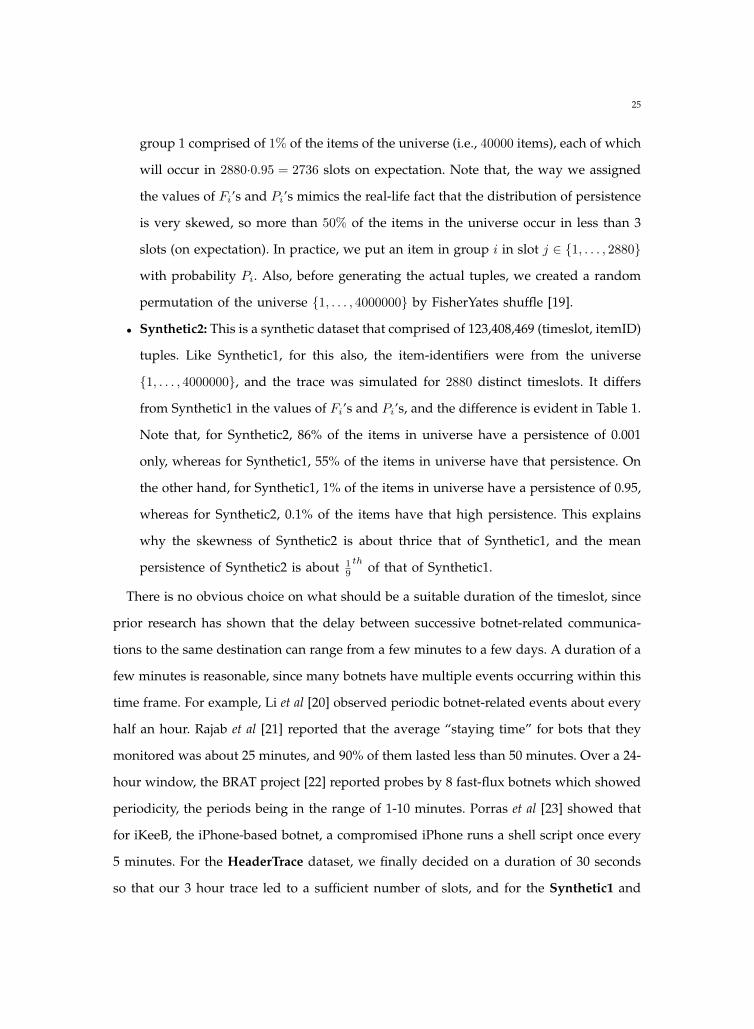
25

group 1 comprised of 1% of the items of the universe (i.e., 40000 items), each of which

will occur in 2880·0.95 = 2736 slots on expectation. Note that, the way we assigned

the values of Fi’s and Pi’s mimics the real-life fact that the distribution of persistence

is very skewed, so more than 50% of the items in the universe occur in less than 3

slots (on expectation). In practice, we put an item in group i in slot j ∈ 1, . . . , 2880

with probability Pi. Also, before generating the actual tuples, we created a random

permutation of the universe 1, . . . , 4000000 by FisherYates shuffle [19].

• Synthetic2: This is a synthetic dataset that comprised of 123,408,469 (timeslot, itemID)

tuples. Like Synthetic1, for this also, the item-identifiers were from the universe

1, . . . , 4000000, and the trace was simulated for 2880 distinct timeslots. It differs

from Synthetic1 in the values of Fi’s and Pi’s, and the difference is evident in Table 1.

Note that, for Synthetic2, 86% of the items in universe have a persistence of 0.001

only, whereas for Synthetic1, 55% of the items in universe have that persistence. On

the other hand, for Synthetic1, 1% of the items in universe have a persistence of 0.95,

whereas for Synthetic2, 0.1% of the items have that high persistence. This explains

why the skewness of Synthetic2 is about thrice that of Synthetic1, and the mean

persistence of Synthetic2 is about 19

th of that of Synthetic1.

There is no obvious choice on what should be a suitable duration of the timeslot, since

prior research has shown that the delay between successive botnet-related communica-

tions to the same destination can range from a few minutes to a few days. A duration of a

few minutes is reasonable, since many botnets have multiple events occurring within this

time frame. For example, Li et al [20] observed periodic botnet-related events about every

half an hour. Rajab et al [21] reported that the average “staying time” for bots that they

monitored was about 25 minutes, and 90% of them lasted less than 50 minutes. Over a 24-

hour window, the BRAT project [22] reported probes by 8 fast-flux botnets which showed

periodicity, the periods being in the range of 1-10 minutes. Porras et al [23] showed that

for iKeeB, the iPhone-based botnet, a compromised iPhone runs a shell script once every

5 minutes. For the HeaderTrace dataset, we finally decided on a duration of 30 seconds

so that our 3 hour trace led to a sufficient number of slots, and for the Synthetic1 and

26

TABLE 1: Distribution of persistence for all datasets

Partition of universe Synthetic1 Synthetic2 HeaderTraceFi Pi Fi Pi

i = 1 0.01 0.95 0.001 0.95i = 2 0.02 0.75 0.002 0.75i = 3 0.03 0.55 0.003 0.55i = 4 0.04 0.35 0.004 0.35i = 5 0.05 0.25 0.005 0.25i = 6 0.06 0.15 0.006 0.15i = 7 0.07 0.1 0.007 0.1i = 8 0.08 0.05 0.01 0.05i = 9 0.09 0.01 0.1 0.01i = 10 0.55 0.001 0.862 0.001∑10i=1 Fi 1 1

Size of universe 4,000,000 4,000,000 2,047,953Exp. packets 1,024,704,000 123,402,240

Actual packets 1,024,680,418 123,408,469 885,055,227Mean persistence 0.089 0.01 0.0177

Third moment of persistence (m3) 0.0105 0.0014 0.0043Variance of persistence (m2) 0.015 0.0019 0.006

Skewness of persistence (m3/m23/2) 5.67 17.17 9.28

Synthetic2 datasets, we chose the length to be 15 minutes. This helped us evaluate the

scalability of our algorithm with increasing number of timeslots, and also to experiment

with different slot-lengths. With the above setting of parameters, for the HeaderTrace

and the synthetic datasets, we had reasonably large number of timeslots (360 and 2880

respectively) as well as a large number of packets per timeslot.

The algorithms were implemented in C++ using the STL extensions. For the hash

functions in the small space algorithm (Algorithm 5), we used an endian-neutral imple-

mentation of the Murmur Hash algorithm [24], which is generally considered to generate

high quality hash outputs.

We obtained the ground truth about the persistence of individual items (IP addresses

for HeaderTrace) by running the naive algorithm over the input data streams. Note that,

although for the synthetic datasets, we determined which item will have how much

persistence, the actual data was generated by a probabilistic process, so we still needed

to collect the actual persistence values of the items. In the process, for the HeaderTrace

dataset, we discovered that a large fraction of the windows did not contain many per-

27

sistent items. On such windows, our algorithm will run in a space-efficient manner, but

we did not consider these windows since there would not be enough data for a fair

comparison.

To simplify the presentation, on HeaderTrace, we focus on 11 specific “query” windows:

these are [1, 100], [26, 125], [51, 150], . . . , [251, 350]. On both the synthetic datasets, the query

windows are [1, 288], [289, 576], . . . , [2593, 2880], so on these two, the time-duration of the

query window was 288·15/60 = 72 hours. We use window [a, b] to denote the window

of all timeslots starting from a till b (both endpoints included).

On HeaderTrace, we found that the cumulative distribution of the persistence values

in the dataset was highly skewed, for every query window that we tried. We present the

CDF of persistence for three out of the 11 query windows: [1, 100], [101, 200] and [201, 300]

in Figure 1, but all the 11 query windows showed similar pattern. For example, in the

[101, 200] window, more than 50% IP addresses occur in 1 slot only, and 95% of the IP

addresses occur in 20 or less slots. This confirms the utility of an algorithm like ours,

which requires less space when items have lower average persistence.

We made the distribution of Synthetic1 less skewed (Figure 2) than that of HeaderTrace

(skewnesses are respectively 5.67 and 9.28, as shown in Table 1), to construct Synthetic1

as an adversarial input dataset, and found the results for HeaderTrace better than those

for Synthetic1. In Figure 2, we present the CDF for only one query window as the

distributions are identical across all windows, because of the way the dataset is generated.

Then again, we constructed Synthetic2 as the dataset with highest skew (17.17, as in

Table 1) of all three, and thus it shows some improvement over Synthetic1, as we explain

later.

Metrics: The following metrics were used. For parameter α, an item that is not α-

persistent, as per the definition of α-persistence given in Definition 2.2, is called “tran-

sient”. Note that this implies that an item with persistence between αn and (α − ε)n is

also treated as transient.

The False Negative Rate (FNR) is defined as the ratio of the number of α-persistent items

that were not reported by the small space algorithm to the total number of α-persistent

28

items.

The False Positive Rate (FPR) is defined as the ratio of the number of transient items

that were reported as persistent by the algorithm to the total number of transient items.

The Space Compression (SC) is defined as the ratio of the number of tuples stored by

the naive algorithm to the number of tuples stored by the small space algorithm.

The Physical Space Compression (PSC) is defined as the maximum Resident Set Size of

the naive algorithm to that of the small-space algorithm. The Resident Set Size (RSS) is

the part of the memory of a process that is held in RAM. We do not use the Virtual Set

Size (VSZ) because that includes the swapped out memory for a process.

The notion of Space Compression (SC) is a logical one, and for the sliding window

version of the problem (Problem 3), we were interested in the number of tuples of the

form (d, t, ·, ·), as referred to in Algorithms 5 to 7.

In the actual implementation, for each distinct item d, we maintained a sorted list (of

variable size) of (t′, nd,t′) tuples, ordered by t′, where nd,t′ indicates in how many distinct

slots d has appeared since its appearance in slot t′. The sorted list helped us to check by

binary-search if an item d has occurred in a given slot t′. When d appears in a slot t′ it

has not appeared in before, the tuple (t′, nd,t′) is initialized only if h(d, t′) < τ . Note that

td,t′ - the last timeslot d has appeared in since its appearance in t′, does not depend on

t′, and hence we maintained a single copy of this variable for each item d.

Since the resident set is specific to a process run by the operating system, for computing

the Physical Space Compression (PSC), for each combination of α and ε, we actually

created a new process so that the resident set is created afresh. We used the getrusage()

function of C++ to measure the maximum resident set size of the process in kilobytes.

However, we are more interested in knowing by how much our algorithm reduces the

memory usage compared to a naive algorithm, and how it varies with the tunable

parameters of the algorithm. We expect the Physical Space Compression for (α, ε′) to

be higher than that for (α, ε) when ε′ > ε (because τ is lower for ε′), but we found that

because of the way memory allocation algorithms work, if the algorithm runs first for

(α, ε) and then for (α, ε′) (using the same process), then, the memory allocated for (α, ε) is

29

enough to accomodate the algorithm for (α, ε′), and the space-saving due to (α, ε′) does

not get reflected.

Note that both the numerator and the denominator of each metric depend on the

query window [c− n+ 1, c] (n is the window length). To measure the ratios, we ran the

small-space algorithm on the query windows defined previously and in each window,

recorded all the items that were marked as persistent by the algorithm. The only source

of randomness in each run is the output of the Murmur Hash function and we ran each

simulation thrice using different seeds (we saw very minor variation in the results when

different seeds were used.) Thus, for each parameter setting we had 11 × 3 data points

for HeaderTrace, and 10 × 3 data points for both the synthetic datasets, and in each

we recorded the false positives, the false negatives, and the number of tuples that were

tracked. The ratios computed (by comparing to the naive algorithm) are then averaged

across all the runs.

0 0.2 0.4 0.6 0.8 10.4

0.5

0.6

0.7

0.8

0.9

1

Persistence

CD

F

CDF for [1,100]

CDF for [101,200]

CDF for [201,300]

Fig. 1: CDF of persistence values from 3 windows for the HeaderTrace dataset

Observations along metrics:

For every value of α, the False Negative Rate (Figure 4a for HeaderTrace, Figure 5a

for Synthetic1 and Figure 6a for Synthetic2) increases as ε increases, which is expected.

However, although Lemma 3.6 bounds the False Negative Rate to 1e2 = 13%, the algorithm

performed much better in practice - we found that even for α = 0.3 and ε = 0.21, the FNR

30

0.0 0.2 0.4 0.6 0.8 1.0

0.2

0.4

0.6

0.8

1.0

Persistence

CD

F

Fig. 2: CDF of persistence values from the [1,288] window for the Synthetic1 dataset

0.0 0.2 0.4 0.6 0.8 1.0

0.6

0.7

0.8

0.9

1.0

Persistence

CD

F

Fig. 3: CDF of persistence values from the [1,288] window for the Synthetic2 dataset

was as low as 2% for HeaderTrace and ∼3.5% for both the synthetic datasets. Note that

εα is a relative measure of error tolerance in α, which in this case is as high as 70%. The

highest FNR we ever got was less than 10% for HeaderTrace, less than 12% for Synthetic1

and 12.7% for Synthetic2. However, for all the three datasets, this was for the highest

setting of α (α = 0.9) - the number of false negatives for this were higher than for the

other settings, for similar values of ε. One possible reason is that for α = 0.9, an item that

was 0.9-persistent had persistence very close to 0.9n. Whereas, many of the items that

31

0 0.1 0.2 0.3 0.4 0.5 0.6 0.70

0.01

0.02

0.03

0.04

0.05

0.06

0.07

0.08

0.09

0.1

ε

Fa

lse

Ne

ga

tive

Ra

te (

FN

R)

α = 0.3

α = 0.5

α = 0.7

α = 0.9

(a) Variation of FNR with α and ε

0 0.1 0.2 0.3 0.4 0.5 0.6 0.70

0.005

0.01

0.015

0.02

0.025

0.03

ε

Fa

lse

Po

sitiv

e R

ate

(F

PR

)

α = 0.3

α = 0.5

α = 0.7

α = 0.9

(b) Variation of FPR with α and ε

0 0.1 0.2 0.3 0.4 0.5 0.6 0.70

5

10

15

20

25

30

35

ε

Space C

om

pre

ssio

n R

atio

α = 0.3

α = 0.5

α = 0.7

α = 0.9

(c) Variation of SC with α and ε

0 0.1 0.2 0.3 0.4 0.5 0.6 0.71

2

3

4

5

6

7

ε

Physic

al S

pace C

om

pre

ssio

n R

atio

α = 0.3

α = 0.5

α = 0.7

α = 0.9

(d) Variation of PSC with α and ε

Fig. 4: Trade-off between accuracy and space for the small-space algorithm over sliding windowsfor the HeaderTrace dataset. Each point in each plot is an average from 33 data points - 3 runsover 11 query windows each. Note that the Y-axis is different for each plot. Also, for each valueof α, the values of ε range from 0.1α to 0.7α.

were 0.3-persistent had persistence values that were much larger than 0.3n. Items that

have persistence values close to the threshold, but higher than it, have a greater chance

of not being reported than items whose persistence values are far above the threshold.

Hence, the false negative ratio for α = 0.9 is a little higher.

The False Positive Rate, similar to the False Negative Rate, shows (Figure 4b for Head-

erTrace, Figure 5b for Synthetic1 and Figure 6b for Synthetic2) an increasing trend as ε

increases. The maximum FPR was 2.69% for HeaderTrace and 2.2% for Synthetic2 (both

for α = 0.3 and ε = 0.21). Moreover, all of Figures 4b, 5b and 6b show that for the same

value of ε, the FPR is lower for higher values of α. The possible reason is that when α

32

0 0.1 0.2 0.3 0.4 0.5 0.6 0.70

0.02

0.04

0.06

0.08

0.1

0.12

ε

Fa

lse

Ne

ga

tive

Ra

te (

FN

R)

α = 0.3

α = 0.5

α = 0.7

α = 0.9

(a) Variation of FNR with α and ε

0 0.1 0.2 0.3 0.4 0.5 0.6 0.70

0.02

0.04

0.06

0.08

0.1

0.12

0.14

0.16

ε

Fa

lse

Po

sitiv

e R

ate

(F

PR

)

α = 0.3

α = 0.5

α = 0.7

α = 0.9

(b) Variation of FPR with α and ε

0 0.1 0.2 0.3 0.4 0.5 0.6 0.70

10

20

30

40

50

60

70

80

90

100

ε

Spa

ce

Co

mpre

ssio

n R

atio

α = 0.3

α = 0.5

α = 0.7

α = 0.9

(c) Variation of SC with α and ε

0 0.1 0.2 0.3 0.4 0.5 0.6 0.71.5

2

2.5

3

3.5

4

4.5

ε

Physic

al S

pace C

om

pre

ssio

n R

atio

α = 0.3

α = 0.5

α = 0.7

α = 0.9

(d) Variation of PSC with α and ε

Fig. 5: Trade-off between accuracy and space for the small-space algorithm over sliding windowsfor the Synthetic1 dataset. Each point in each plot is an average from 30 data points - 3 runs over10 query windows each. The Y-axis is different for each plot. For each value of α, the values of εrange from 0.1α to 0.7α.

is very high (e.g. 0.9), most items have persistence much lower than αn (as is evident

from the CDFs in Figures 1 and 2), hence are very unlikely to cross the threshold T in

Algorithm 7.

The (Logical) Space Compression increases linearly with ε (Figures 4c for HeaderTrace,

5c for Synthetic1 and 6c for Synthetic2), and we found the Space Compression is close

to 1τ = εn

2 , for all values of α and all three datasets. This is expected since the naive

algorithm creates a new tuple for an item everytime it appears in a different slot - where

the small-space algorithm creates a tuple with probability τ only. For α = 0.9, with

ε = 0.63, the logical space compression was as high as 32 for HeaderTrace, and as high

33

0 0.1 0.2 0.3 0.4 0.5 0.6 0.70

0.02

0.04

0.06

0.08

0.1

0.12

ε

Fa

lse

Ne

ga

tive

Ra

te (

FN

R)

α = 0.3

α = 0.5

α = 0.7

α = 0.9

(a) Variation of FNR with α and ε

0 0.1 0.2 0.3 0.4 0.5 0.6 0.70

0.005

0.01

0.015

0.02

0.025

ε

Fa

lse

Po

sitiv

e R

ate

(F

PR

)

α = 0.3

α = 0.5

α = 0.7

α = 0.9

(b) Variation of FPR with α and ε

0 0.1 0.2 0.3 0.4 0.5 0.6 0.70

10

20

30

40

50

60

70

80

90

100

ε

Spa

ce

Com

pre

ssio

n R

atio

α = 0.3

α = 0.5

α = 0.7

α = 0.9

(c) Variation of SC with α and ε

0 0.1 0.2 0.3 0.4 0.5 0.6 0.71.5

2

2.5

3

3.5

4

ε

Physic

al S

pace C

om

pre

ssio

n R

atio

α = 0.3

α = 0.5

α = 0.7

α = 0.9

(d) Variation of PSC with α and ε

Fig. 6: Trade-off between accuracy and space for the small-space algorithm over sliding windowsfor the Synthetic2 dataset. Other details are same as Synthetic1.

as 91 for Synthetic1 and ∼100 for Synthetic2. The higher Space Compression for the

synthetic datasets compared to HeaderTrace is justified by the larger value of the window

length n (288 as opposed to 100). For higher values of α, we could achieve better Space

Compression as the tolerance ε could be made higher while keeping the false positives

and the false negatives small enough.

Like its logical counterpart, the Physical Space Compression also increases with ε (Fig-

ure 4d for HeaderTrace, 5d for Synthetic1 and 6d for Synthetic2), and for each distinct

value of α, the Physical Space Compression grows almost linearly with ε. For higher

values of α, we could achieve better Space Compression as the tolerance ε could be made

higher. While the size of the HeaderTrace dataset was 58 GB, the maximum resident set

34

0 0.05 0.1 0.15 0.2 0.25 0.3 0.35 0.40

0.2

0.4

0.6

0.8

1

1.2

1.4

1.6

1.8

2x 10

6

ε

Ph

ysic

al M

em

ory

Small Space

Naive

(a) Variation of actual memory used with ε

0.05 0.1 0.15 0.2 0.25 0.3 0.35

ε

#P

ers

iste

nt item

s

050000

150000

250000

#True Positives

#False Positives

(b) Variation of number of true positives and falsepositives with ε

0.05 0.1 0.15 0.2 0.25 0.3 0.35

ε

#Tra

nsie

nt item

s

0500000

1500000

#True Negatives

#False Negatives

(c) Variation of number of true negatives and falsenegatives with ε

Fig. 7: The variation of the physical memory taken, the number of true positives, false positives,true negatives and false negatives with ε for the Synthetic1 dataset. All the plots are for α = 0.5and the query window [2593, 2880]. So, each point in each plot is an average from 3 data pointscorresponding to the 3 different seed values (10, 20, 30). Note that the horizontal line in the firstplot represents the actual memory taken by the naive algorithm, and hence does not vary with ε.The Y-axis is different for each plot. The values of ε range from 0.1α to 0.7α.

size of the naive algorithm went up to 3 GB (at the query window [251,350]), whereas

for typical parameters like α = 0.5 and ε = 0.35, the small-space algorithm took less than

15

th (600 MB) memory (on average) compared to the naive algorithm. For Synthetic1, the

dataset size was 12 GB, the maximum resident set size of the naive algorithm went up to

1.8 GB, whereas for α = 0.5 and ε = 0.35, the small-space algorithm took space between

350 and 500 MB. For Synthetic2, the dataset size was 1.5 GB, the maximum resident set

size of the naive algorithm went up to 736 MB, whereas for α = 0.5 and ε = 0.35, the

small-space algorithm took space between 140 and 200 MB.

35

10 20 300

0.2

0.4

0.6

0.8

1

1.2

1.4

1.6

1.8

2x 10

6

seed

Physic

al M

em

ory

Small Space

Naive

(a) Variation of actual memory used with seed

10 20 30

seed

#P

ers

iste

nt item

s

050000

150000

250000

#True Positives

#False Positives

(b) Variation of number of true positives and falsepositives with seed

10 20 30

seed

#Tra

nsie

nt item

s

0500000

1500000

2500000

#True Negatives

#False Negatives

(c) Variation of number of true negatives and falsenegatives with seed

Fig. 8: The variation of the physical memory taken, the number of true positives, false positives,true negatives and false negatives with the seed of the random number generator for the Synthetic1dataset. All the plots are for α = 0.5, ε = 0.15 and the query window [2593, 2880]. Note that thehorizontal line in the first plot represents the actual memory taken by the naive algorithm, andhence does not vary with the seed. The Y-axis is different for each plot. The values of the seedused are 10, 20 and 30.

Variation with ε, seed and query window: Figures 7a through 9c take a closer look at

some of the absolute numbers (actual memory used, number of true and false positives,

number of true and false negatives) rather than ratios for the Synthetic1 dataset, and

show how they vary with ε, the seed value of the random number generator and the

different query windows. Figure 7a shows how the physical memory (in KB) varies with

ε for α = 0.5 and the query window [2593, 2880]. Since the memory taken by the naive

algorithm does not depend on α or ε, it is constant throughout at 1.86 GB, and the memory

36

288 576 864 1152 1440 1728 2016 2304 2592 28800

0.2

0.4

0.6

0.8

1

1.2

1.4

1.6

1.8

2x 10

6

Query window

Ph

ysic

al M

em

ory

Small Space

Naive

(a) Variation of actual memory used with querywindow

288 576 864 1440 2016 2592

Query window

#P

ers

iste

nt item

s

050000

150000

250000

#True Positives

#False Positives

(b) Variation of number of true positives and falsepositives with query window

288 576 864 1440 2016 2592

Query window

#P

ers

iste

nt item

s

0500000

1500000

2500000

#True Negatives

#False Negatives

(c) Variation of number of true negatives and falsenegatives with query window

Fig. 9: The variation of the physical memory taken, the number of true positives, false positives,true negatives and false negatives with the query window for the Synthetic1 dataset. All the plotsare for α = 0.5, ε = 0.15 and seed = 10. Note that the horizontal line in the first plot representsthe actual memory taken by the naive algorithm, and shows slight increase with the progress oftime (increasing query window number). The Y-axis is different for each plot. The query windowsare [1, 288], [289, 576], . . . , [2593, 2880] and the values on the X-axis are the endpoints of the querywindows.

taken by the small space algorithm falls from 800 MB to 500 MB as ε increases from 0.05

to 0.35.

In Figure 7b, the actual number of persistent items in the window [2593, 2880] is

constant at 235,353; and we can see that with increasing ε, the number of true positives

reduces only a little, remaining very close to the number of actual persistent items

throughout. The number of false positives is as low as ∼3,600 when ε = 0.05, and for

typical values of ε (e.g., 0.15) that will probably be used in practice for a problem like

37

this, the number of false positives is ∼25k.

In Figure 7c, the actual number of transient items in the window [2593, 2880] is constant

at ∼2.1m; and we can see that with increasing ε, the number of true negatives reduces

only a little, remaining very close to the number of actual transient items throughout.

The number of false negatives is as low as ∼2,200 when ε = 0.05, and even when ε is as

high as 0.35, the number of false negatives increases only to ∼14k. Note that, for many

practical applications, it is important to keep the number/rate of false negatives much

lower compared to the number/rate of false positives, and comparing Figure 7b and 7c

shows that our algoithm meets that criterion.

Figure 8a shows how the physical memory (in KB) varies with the seed of the random

number generator for α = 0.5, ε = 0.15 and the query window [2593, 2880]. Since the

memory taken by the naive algorithm does not depend on the seed of the random number

generator, it is constant throughout at 1.86 GB, and the memory taken by the small space

algorithm also remains practically constant at ∼593MB, which justifies averaging the

actual memory footprint over the 3 different seed values.

In Figure 8b, the actual number of persistent items in the window [2593, 2880] is

constant at 235,353; and we can see that with change in the seed, the number of true

positives remains practically constant at ∼227k, and so does the number of false positives

at ∼26k.

In Figure 8c, the actual number of transient items in the window [2593, 2880] is constant

at ∼2.1m; and we can see that with change in the seed, the number of true negatives

remains practically constant at ∼2.07m, and so does the number of false negatives at

∼7.8k.

Figure 9a shows how the physical memory (in KB) varies with the query window

for α = 0.5 and ε = 0.15, the seed of the random number generator being 10. Unlike

Figure 7a or Figure 8a, the physical memory depends on the number of distinct items

in the window, and although we generated the items uniformly across the slot range

[1, 2880], we see it increased gradually with increasing slot number. However, while the

space taken by the naive algorithm varied from 1.5 GB to 1.86 GB, the space taken by

38

the small-space algorithm varied from ∼400 MB to ∼600MB.

Figure 9b shows how the number of persistent items varies with the query window for

α = 0.5 and ε = 0.15, the seed of the random number generator being 10. Since for the

Synthetic1 dataset, each persistent item was distributed uniformly across the slot range

[1, 2880], the actual number of persistent items across the different windows was almost

constant at ∼235k; and we can see that with change in the query window, the number

of true positives also remains practically constant at ∼227k, and so does the number of

false positives at ∼26k.

Figure 9c shows how the number of transient items varies with the query window

for α = 0.5 and ε = 0.15, the seed of the random number generator being 10. For the

Synthetic1 dataset, like the persistent items, each transient item was also distributed

uniformly across the slot range [1, 2880], hence the actual number of transient items across

the different query windows is practically constant at ∼2.1m; and we can see that with

change in the query window, the number of true negatives remains practically constant

at ∼2.07m, and so does the number of false negatives at ∼7.8k.

The small variation in the actual memory used, the number of true and false positives

and the number of true and false negatives by the small-space algorithm, as shown in

Figures 8a through 9c justifies our averaging of these quantities across the different seed

values and query windows.

Comparsion among three datasets: The FPR for HeaderTrace was much lower than that

for Synthetic1 at comparable points, e.g., at α = 0.3, ε = 0.21 and in comparable query

windows, for Synthetic1, the FPR is 16%, whereas for HeaderTrace, the FPR is 2.7%. For

Synthetic1, at an identical query window, there are ∼300k false positives out of ∼1931k

transient items, and for HeaderTrace, there are ∼21k false positives out of ∼802k transient

items. The lower FPR for HeaderTrace probably arises out of the fact that the CDF curve

(Figure 1) grows more steeply than the CDF curve for Synthetic1 (Figure 2), so the fraction

of items whose persistence come anywhere close to 0.3 is much less. To demonstrate the

difference among the three datasets, we present the 93rd percentile value of persistence

for each. For HeaderTrace, there are total ∼829k distinct items in the window [251,350],

39

but ∼770k of these items occur in 10 or less slots out of 100, i.e., the 93rd percentile value

of persistence is 10%. As a comparison, for Synthetic1, there are total ∼2330k distinct

items in the window [2593, 2880], but ∼2167k of these items occur in 161 or less slots

out of 288 (161/288 = 56%), i.e., the 93rd percentile value of persistence is 56%. But then

again, for Synthetic2, the FPR improves significantly over Synthetic1 - for α = 0.3 and

ε = 0.21, Synthetic2 gives an FPR of 2.2% in pretty much all query windows - so the

FPR becomes comparable to that of HeaderTrace. To compare with Synthetic1, there are

∼1394k distinct items in the window [2593, 2880], but ∼1296k of them occur in 28 or less

slots out of 288, i.e., the 93rd percentile value of persistence is 9.7% (see Figure 3). The

reason for lower FPR for Synthetic2 is similar to that for HeaderTrace. This shows that

the FPR improves with skewness of the data, and our algorithm in fact performs well

for datasets with realistic skewness.

The physical memory compression ratio is less for Synthetic1 than for HeaderTrace for

similar reasons - many transient items find room into the sketch for having persistence

close to the threshold. Although the skew for Synthetic2 is more than that of Synthetic1,

it has similar values of logical and physical memory compressions since the proportion

of items from the universe that have similar persistence values bear similar ratios to each

other, e.g., for Synthetic1, 1% of the items have persistence 0.95 and 2% have persistence

0.75; whereas for Synthetic2, 0.1% of the items have persistence 0.95 and 0.2% have

persistence 0.75 (first two rows of Table 1).

In Lemma 3.7, we showed that for a given value of ε and length of sliding window (n),

the expected number of tuples in the sketch is proportional to the sum of the persistence

values of all items appearing in the window (∑d∈D p

cd). Hence, the physical memory taken

should also vary with the sum of the persistence values. We present the following example

to demonstrate this: in the [1, 288] window, the number of distinct items for Synthetic1

and Synthetic2 are respectively ∼2.33m and ∼1.39m, and the sum of persistence values

for Synthetic1 and Synthetic2 respectively are about 20.47×104 and 1.4×104. For α = 0.5

and ε = 0.35, the memory footprints by the small-space algorithm for this combination

of parameters for Synthetic1 and Synthetic2 are respectively 353 MB and 142 MB, so

40

Synthetic1 takes about 2.5 times more memory than Synthetic2.

5 RELATED WORK

A large body of literature on network anomaly detection has focused on detecting volume-

based anomalies, i.e., tracking IPs which send or receive an unusally large volume of

traffic over an interval of time. While volume-based anomaly detection is relevant for

Denial-of-Service type attacks like SYN flood [25], UDP flood [26], Ping flood or P2P

attacks, there are many “stealthy” attacks [27], which can bypass the radar by never

sending traffic in large volume, yet remaining active over long windows in time, and

probing the target network/host once in a while. For example, port scans [5] look for

open ports on remote hosts that have applications with known vulnerabilities deployed

on those ports; bots installed on compromised hosts in a botnet keep on communicating

with the C&C server, etc. Our work differs from these in that persistent items may not

result in large volumes of traffic and may escape detection by a volume-based system.

It is interesting to compare how algorithmic techniques for identifying heavy-hitters (or

“frequent items”) may work for the problem of identifying persistent items. Broadly, the

techniques in the literature can be classified into “counter-based”, “quantile algorithms”,

“sketches”, or “random sampling-based” (see [28]). Counter-based techniques such as

the Misra-Gries algorithm [7], and the “Space-Saving” algorithm [29] rely on maintaining

per-item counters for counting the number of occurrences of each item that has been

currently identified as being frequent; these counters are occasionally decremented to

ensure that the space taken by the data structure is small. The difficulty in using this

technique for our problem is that it is not easy to ensure that re-occurrences of the same

item within a timeslot have no effect on the system state. For example, in the Misra-

Gries algorithm, if there is a decrement of the counters between two occurrences of an

item within the same timeslot, it seems hard to ensure that the second occurrence has no

effect on the system state, especially given that the increment due to the first occurrence

may have disappeared from the system (due to the decrement). The same argument

is true for Lossy Counting too [8]. Quantile-based algorithms such as Greenwald and

41

Khanna, or [30], the q-digest [31] view the space of all items as being a bijection with

the set of integers, and associate counts with different ranges in this space of all items.

In the q-digest algorithm, there are no decrements to these counters, so one may use

“distinct counters” such as those by Flajolet-Martin [16], or Gibbons and Tirthapura [15],

or Kane, Nelson, and Woodruff [32], instead of regular counters. Such an approach based

on maintaining distinct counters would not only be more complex than our approach,

but also likely have a greater space complexity, since maintaining distinct counters with a

relative error of ε requires Ω(1/ε2) space [17]. The sketch approach, such as count-sketch

[33] or count-min sketch [12] also maintains multiple counters, each of which is the sum of

many random variables. Replacing each such counter with a distinct counter leads to its

own set of difficulties, one of which is the space complexity of distinct counting, explained

above, and the other being the fact that each distinct counter is only approximate (exact

distinct counting necessarily requires large space [34]), while the analyses in [33] and [12]

rely on the different counters in the data structure being exact.

Finally, our algorithm is inspired by the random sampling approaches based on the

“sample and count” scheme of Alon et al. [34], [35] and the “sticky sampling” algorithm of

Manku and Motwani [8]. Both these algorithms use the following idea: “sample a random

element in the stream, and track reoccurrences of this element exactly”. In these works, the

idea was applied to a different context than ours – sample and count was applied to track

the size of a self-join in limited storage, and sticky sampling was used in the identification

of heavy hitters using limited space. Our algorithm has the following technical differences

when compared with the above works. The sampling of an item is done using a hash

function that is based on the item identifier and the timeslot in which it arrived in. This

hash-based sampling avoids giving greater sampling probability to an item if it occurs

multiple times within the same timeslot. Further, reoccurrences are tracked in such a

way that we do not overcount if the same item appears again in the same timeslot. In

addition, we show how to handle sliding windows using nearly the same space, while

the above works do not address the context of sliding windows. A distinguishing aspect

of our work on sliding windows is that while the extension to sliding windows often

42

requires asymptotically greater space than for the infinite window case (for example, see

Arasu and Manku [36]), in our case the space complexity is asymptotically the same.

Persistence is exploited to detect botnet traffic in [1], using an algorithm that tracked

the state of every distinct item that arrived within the sliding window. Hence the memory

used is of the order of the number of distinct items times the window size, which

is potentially very high. In contrast, our algorithm tracks persistent items using much

smaller space, while giving up some accuracy.

There has been much work in estimating various properties of the frequency distribu-

tion of stream items, including the frequency moments of a stream [34], [37], [32], heavy-

hitters [8], [9], [12], [38], and the entropy [39], [40], [41]. Unlike the set of persistent items,

all the above properties depend only on the frequency distribution of items in the stream

– they are unaffected by re-ordering of the stream elements, or by changing the times at

which the elements arrive. In contrast, the set of persistent items in a stream is affected

by the time and order in which elements arrive.

In a recent work on a temporal property of a stream, Chen et al [42] addressed the

problem of tracking long-duration flows from network streams. They identified flows for

which the difference of timestamps between the first and the last packet in the flow exceed

some threshold d. A flow might continue for a long duration and yet the total number

of bytes sent in the flow may not be high enough to be detected by the heavy-hitter

algorithms; whereas some other flow of shorter duration might qualify as a heavy-hitter

because it sends many more bytes. Clearly, a long-lived flow is not necessarily persistent.

6 CONCLUSION

We formulated the problem of detecting persistent items in a data stream. Our lower bound

result shows that an exact algorithm for the problem, which reports all persistent items,

would need a prohibitively high memory, and is therefore impractical. Subsequently, we

presented an approximate formulation of the problem that explores a tradeoff between

space and accuracy in identifying persistent items. Allocating more memory leads to more

accurate answers and this allows operators to tune their systems appropriately depending

43

on the amount of resources available.

By running simulations of both the naive (exact) and small space algorithms on a real

as well as two synthetic traffic datasets with different skewness, we demonstrate that our

algorithm works very well in practice: for the real trace, it uses up to 85% less space than

the naive (exact) algorithm and incurs a false positive rate (and false negative rate) of

less than 1% (and 4% respectively) for typical values of the parameters. We also see that

false positive rate never exceeds 3% for any parameter setting, while the false negative

rate stays below 5% for all but the most aggressive thresholds for persistence. For the

synthetic trace with low skewness, the small-space algorithm uses up to 80% less space

than the naive one, the false positive rate is less than 2% and the false negative rate

is about 4% for typical parameter values (e.g., α = 0.5 and ε = 0.15). The maximum

false positive rate is less than 3% for the real trace and the synthetic trace with higher

skewness. The empirical false positive and false negative rates, for most parameters, are

much better than the analytical bounds: and our experiment across the three different

datasets shows that the false positive rate improves for data with higher skewness.

REFERENCES

[1] F. Giroire, J. Chandrashekar, N. Taft, E. Schooler, and D. Papagiannaki, “Exploiting temporal persistence

to detect covert botnet channels,” in Proceedings of the 12th International Symposium on Recent Advances in

Intrusion Detection (RAID), 2009, pp. 326–345.

[2] “Google AdWords,” http://www.google.com/ads/adwords2/.

[3] L. Zhang and Y. Guan, “Detecting click fraud in pay-per-click streams of online advertising networks,”

in Proceedings of the 28th IEEE International Conference on Distributed Computing Systems (ICDCS), 2008, pp.

77–84.

[4] S. Guha, J. Chandrashekar, N. Taft, and K. Papagiannaki, “How healthy are today’s enterprise networks?”

in Proceedings of the 8th ACM SIGCOMM Conference on Internet Measurement (IMC), 2008, pp. 145–150.

[5] S. Staniford, J. A. Hoagland, and J. M. McAlerney, “Practical automated detection of stealthy portscans,”

in Journal of Computer Security, 2002, vol. 10, no. 1/2, pp. 105–136.

[6] “Advanced Persistent Threat,” http://www.usenix.org/event/lisa09/tech/slides/daly.pdf.

[7] J. Misra and D. Gries, “Finding repeated elements,” Science of Computer Programming, vol. 2, no. 2, pp.

143–152, 1982.

[8] G. S. Manku and R. Motwani, “Approximate frequency counts over data streams,” in Proceedings of 28th

International Conference on Very Large Data Bases (VLDB), 2002, pp. 346–357.

44

[9] C. Estan and G. Varghese, “New directions in traffic measurement and accounting: Focusing on the

elephants, ignoring the mice,” ACM Transactions on Computer Systems, vol. 21, no. 3, pp. 270–313, 2003.

[10] M. Charikar, K. Chen, and M. Farach-Colton, “Finding frequent items in data streams,” Theoretical Computer

Science, vol. 312, no. 1, pp. 3–15, 2004.

[11] G. Cormode, F. Korn, S. Muthukrishnan, and D. Srivastava, “Diamond in the rough: Finding hierarchical

heavy hitters in multi-dimensional data,” in Proceedings of the ACM SIGMOD International Conference on

Management of Data (SIGMOD), 2004, pp. 155–166.

[12] G. Cormode and S. Muthukrishnan, “An improved data stream summary: the count-min sketch and its

applications,” Journal of Algorithms, vol. 55, no. 1, pp. 58–75, 2005.

[13] S. Venkataraman, D. X. Song, P. B. Gibbons, and A. Blum, “New streaming algorithms for fast detection

of superspreaders,” in Proceedings of the Network and Distributed System Security Symposium (NDSS), 2005,

pp. 149–166.

[14] N. Bandi, D. Agrawal, and A. E. Abbadi, “Fast algorithms for heavy distinct hitters using associative

memories,” in Proceedings of the 27th IEEE International Conference on Distributed Computing Systems (ICDCS),

2007, pp. 6–14.

[15] P. Gibbons and S. Tirthapura, “Estimating simple functions on the union of data streams,” in Proceedings

of the 13th ACM Symposium on Parallel Algorithms and Architectures (SPAA), 2001, pp. 281–291.

[16] P. Flajolet and G. N. Martin, “Probabilistic counting algorithms for database applications,” Journal of

Computer and System Sciences, vol. 31, pp. 182–209, 1985.

[17] P. Indyk and D. Woodruff, “Tight lower bounds for the distinct elements problem,” in Proceedings of the

44th IEEE Symp. on Foundations of Computer Science (FOCS), 2003, pp. 283–288.

[18] CAIDA, “OC48 traces dataset,” https://data.caida.org/datasets/oc48/oc48-original/20020814/5min/.

[19] R. Durstenfeld, “Algorithm 235: Random permutation,” Communications of the ACM, vol. 7, no. 7, p. 420,

1964.

[20] Z. Li, A. Goyal, Y. Chen, and V. Paxson, “Automating analysis of large-scale botnet probing events,” in

Proceedings of the 2009 ACM Symposium on Information, Computer and Communications Security (ASIACCS),

2009, pp. 11–22.

[21] M. A. Rajab, J. Zarfoss, F. Monrose, and A. Terzis, “A multifaceted approach to understanding the botnet

phenomenon,” in Proceedings of the 6th ACM SIGCOMM Conference on Internet Measurement (IMC), 2006,

pp. 41–52.

[22] “Botnet Reporting and Termination,” http://spamtrackers.eu/wiki/index.php/Botnet Reporting.

[23] P. Porras, H. Saidi, and V. Yegneswaran, “An Analysis of the iKeeB (duh) iPhone botnet (worm),” http:

//mtc.sri.com/iPhone/.

[24] A. Appleby, “Murmurhash 2.0,” http://sites.google.com/site/murmurhash/.

[25] “CERT advisory CA-1996-21 TCP SYN flooding and IP spoofing attacks,” http://www.cert.org/advisories/

CA-1996-21.html.

[26] “CERT advisory CA-1996-01 UDP port denial-of-service attack,” http://www.cert.org/advisories/

CA-1996-01.html.

45

[27] Y. Gao, Y. Zhao, R. Schweller, S. Venkataraman, Y. Chen, D. Song, and M.-Y. Kao, “Detecting stealthy

attacks using online histograms,” in International Workshop on Quality of Service, 2007.

[28] G. Cormode and M. Hadjieleftheriou, “Finding frequent items in data streams,” Proceedings of the VLDB

Endowment (PVLDB), vol. 1, no. 2, pp. 1530–1541, 2008.

[29] A. Metwally, D. Agrawal, and A. E. Abbadi, “Efficient computation of frequent and top-k elements in data

streams,” in Proceedings of the 10th International Conference on Database Theory (ICDT), 2005, pp. 398–412.

[30] M. Greenwald and S. Khanna, “Space efficient online computation of quantile summaries,” in Proceedings

of the 20th ACM International Conference on Management of Data (SIGMOD), 2001, pp. 58–66.

[31] N. Shrivastava, C. Buragohain, D. Agrawal, and S. Suri, “Medians and beyond: new aggregation techniques

for sensor networks,” in Proceedings of the 2nd International Conference on Embedded Networked Sensor Systems

(SenSys), 2004, pp. 239–249.

[32] D. M. Kane, J. Nelson, and D. P. Woodruff, “An optimal algorithm for the distinct elements problem,” in

Proceedings of the 29th ACM SIGMOD-SIGACT-SIGART Symposium on Principles of Database Systems (PODS),

2010.

[33] M. Charikar, K. Chen, and M. Farach-Colton, “Finding frequent items in data streams,” in Proceedings of

the 29th International Colloquium Automata, Languages and Programming (ICALP), 2002, pp. 693–703.

[34] N. Alon, Y. Matias, and M. Szegedy, “The space complexity of approximating the frequency moments,”

Journal of Computer and System Sciences, vol. 58, no. 1, pp. 137–147, 1999.

[35] N. Alon, P. B. Gibbons, Y. Matias, and M. Szegedy, “Tracking join and self-join sizes in limited storage,”

Journal of Computer and System Sciences, vol. 64, no. 3, pp. 719–747, 2002.

[36] A. Arasu and G. Manku, “Approximate counts and quantiles over sliding windows,” in Proceedings of

the 23rd ACM SIGMOD-SIGACT-SIGART Symposium on Principles of Database Systems (PODS), 2004, pp.

286–296.

[37] D. P. Woodruff, “Optimal space lower bounds for all frequency moments,” in Proceedings of the 15th Annual

ACM-SIAM Symposium on Discrete Algorithms (SODA), 2004, pp. 167–175.

[38] L.-K. Lee and H. F. Ting, “A simpler and more efficient deterministic scheme for finding frequent items

over sliding windows,” in Proceedings of the 25th ACM SIGACT-SIGMOD-SIGART Symposium on Principles

of Database Systems (PODS), 2006, pp. 290–297.

[39] A. Lall, V. Sekar, M. Ogihara, J. Xu, and H. Zhang, “Data streaming algorithms for estimating entropy of

network traffic,” in Proceedings of the Joint International Conference on Measurement and Modeling of Computer

Systems (SIGMETRICS/Performance), 2006, pp. 145–156.

[40] A. Chakrabarti, K. D. Ba, and S. Muthukrishnan, “Estimating entropy and entropy norm on data streams,”

in Proceedings of the 23rd Annual Symposium on Theoretical Aspects of Computer Science (STACS), 2006, pp.

196–205.

[41] G. Nychis, V. Sekar, D. G. Andersen, H. Kim, and H. Zhang, “An empirical evaluation of entropy-based

traffic anomaly detection,” in Proceedings of the 8th ACM SIGCOMM Conference on Internet Measurement

(IMC), 2008, pp. 151–156.

46

[42] A. Chen, Y. Jin, and J. Cao, “Tracking long duration flows in network traffic,” in Proceedings of the 29th

IEEE International Conference on Computer Communications (INFOCOM), 2010, pp. 206–210.