1

SIMULATION – PART III

Application to Risk Management

2

An Introduction toSimulation and Crystal Ball

(using an example that is an extension of the classic Newsboy Problem)

For this portion of the session, the learning objectives are:

Learn the meaning of Simulation.

Learn the “basics” of using Crystal Ball, an add-in to Excel that enables simulation with a spreadsheet.

Learn how to apply Crystal Ball to a scenario that is an extension of the classic Newsboy Problem.

3

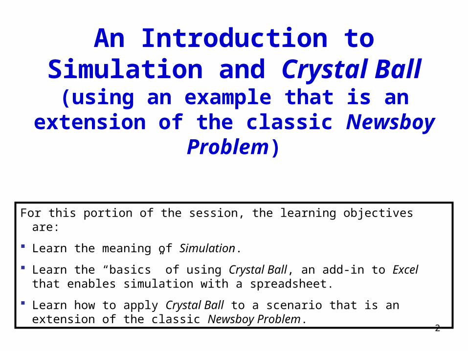
GENERAL PRINCIPLES OF SIMULATION A simulation is an experiment in which we attempt to understand how

something will behave in reality by imitating its behavior in an artificial environment that approximates reality as closely as possible. (In this course, the artificial environment will be an Excel spreadsheet within a computer.)

Within this artificial environment, a simulation conducts an experiment that would be too costly and too time-consuming to conduct in reality. A simulation uses “funny money” and just a few minutes (or seconds) of time.

Because a simulation is based on random numbers, any value obtained from a simulation is only an estimate, that is, only an approximation of the true value.

Because a simulation is based on random numbers, obtaining accurate estimates requires a simulation with a very large number of “trials” (or “runs” or “iterations”).

Because a simulation requires a very large number of trials, a simulation is best conducted on a computer.

4

Below is an example of the classic Newsboy Problem:

At a corner newsstand in Haasville, Randy Hurst sells copies of a daily newspaper for 25¢. At the beginning of each day, Randy buys papers from the local distributor for 10¢ each. According to the contract with his distributor, if Randy runs out of papers during the day, he cannot reorder. Furthermore, if he ends the day with a surplus, his rebate from the distributor is only 4¢ per unsold paper. Because Randy is uncertain about how many papers he will sell, he is uncertain about the number of papers to buy from the distributor. On one hand, if Randy buys more papers than he sells, he has lower profit because the rebate for each unsold paper is less than he paid. On the other hand, if Randy runs out of papers during the day, he has lower profit because of lost sales. Assuming Randy estimates that the daily number of papers he will sell has a Normal Probability Distribution with a mean of 500 and a standard deviation of 30, what should be Randy’s daily purchase quantity?

The distinguishing characteristics of the Newsboy Problem are: The problem involves only a single time period. The item is purchased at the beginning of the period, and, if a stock-out occurs

during the period, there is no opportunity to reorder the item. The problem involves an item that, at the end of the period, either spoils or

becomes obsolete. Therefore, at the end of the period, the item has a salvage price (“dumping price”) that is less than the item’s selling price during the period.

During the period, the item’s demand is a random variable.

5

What is another product whose sale is similar to a Newsboy Problem?

Christmas trees ordered by a retailer from his/her wholesaler.

Chocolate truffles made by a candy manufacturer for Valentine’s Day.

Red roses purchased by a florist from its supplier.

Fresh sourdough baguettes baked at a bakery.

Slices of fresh Ahi tuna ordered by restaurant from its supplier.

A particular type of card made by card manufacturer for Mother’s Day.

6

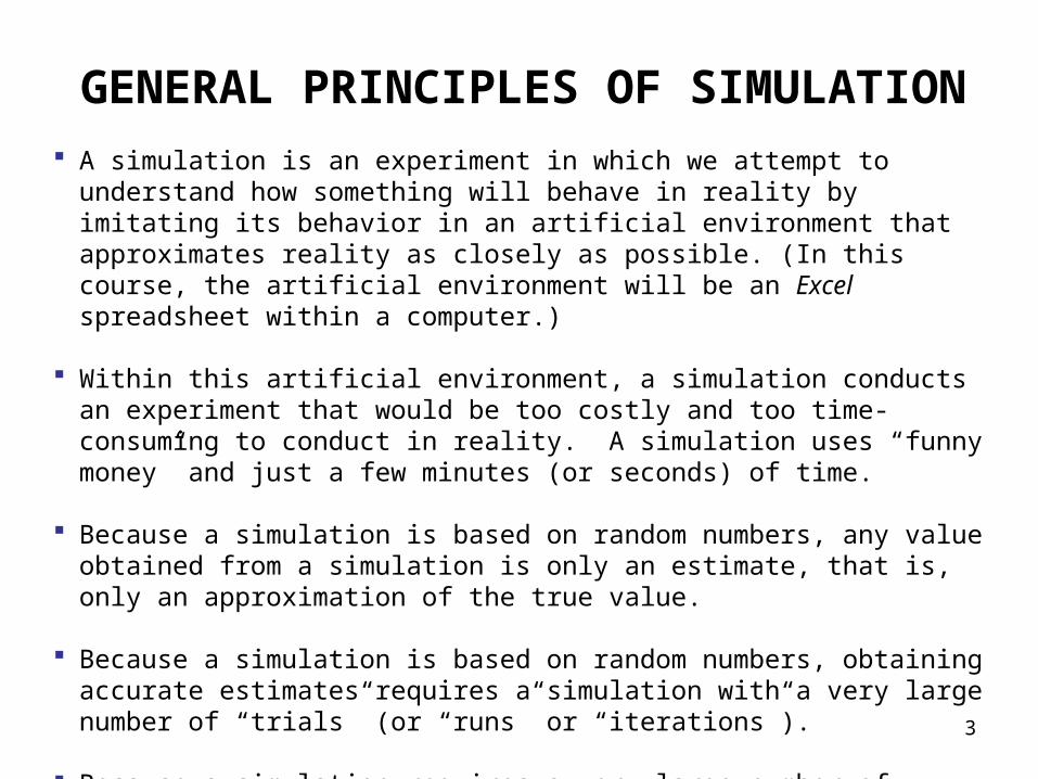
Instead of considering the (one-period) Newsboy Problem, we will consider the following three-period extension of the Newsboy Problem:

Sequoia’s Optimal Production Quantity Problem

For one of its products, Sequoia Computers plans to produce 25,000 units at aproduction cost of $10 per unit. This production quantity must last (with no possibility to increase) through three distinct selling seasons:

Primary Selling Season. During the primary selling season, the unit selling price is $13. Demand during the primary season has a Normal Probability Distribution with a mean of 20,000 and a standard deviation of 4000.

Secondary Selling Season. During the secondary selling season, the unit selling price is $12. Demand during the secondary season has a Normal Probability Distribution with a mean of 5000 and a standard deviation of 1000.

Tertiary Selling Season. During the tertiary selling season, the unit selling price is $8. During the tertiary season, Sequoia can sell any remaining inventory up to a maximum of 2500.

Sequoia wants to estimate the following:The mean and standard deviation of the profit.The probability that profit will fall within the interval of $30,000 to $60,000.The lower 10% “tail”, that is, a value v such that Pr{Profit <= v} = 0.10.

7DefineAssumption

DefineDecision

DefineForecast

Copy Data Paste Data Run Preferences

Start Simulation

Stop Simulation

Reset Simulation

Single Step

Forecast Charts Create Report

New Menu Selections

OVERVIEW OF CRYSTAL BALLAfter launching Crystal Ball, you will see the following menu and toolbars, where the three menu selections and the lower toolbar have been added-in to Excel. Crystal Ball permits three types of cells:

Assumption Cells: Each Assumption Cell contains a value about which you are uncertain. (Think of the Assumption Cells as the decision problem’s independent variables or inputs.)

Forecast Cells: Each Forecast Cell is one of the spreadsheet’s “bottom lines” and contains a formula that refers directly or indirectly to at least one of the Assumption Cells. (Think of the Forecast Cells as the decision problem’s dependent variables or outputs.)

Decision Cells: Each Decision Cell is under control of the decision maker and contains a value from of a set of alternative values.

8

WHEN USING CRYSTAL BALL FOR THE FIRST TIME

When using Crystal Ball for the first time, I recommend that you exercise the option of having Assumption Cells, Forecast Cells, and Decision Cells highlighted -- each type of cell in a different color and/or pattern. To do so, choose the Define, Cell Preferences menu selection and successively choose your desired “feng shui”. My choices are green Assumption Cells, magenta Forecast Cells, and yellow Decision Cells (with no patterns). Below is the screen shot for “Assumptions”, with there being similar screens for “Decision Variables” and Forecasts”.

9

Step 1: Construct the Spreadsheet. Design and construct the spreadsheet in the usual manner, temporarily ignoring any uncertainty and instead entering into an Assumption Cell a constant equal to either the mean or the “most likely” value.

10DefineAssumption

Step 2: Define Each Assumption Cell. To define an Assumption Cell, proceed as follows:

After clicking the cell, click the toolbar’s Define Assumption icon to:(1) select from the Distribution Gallery the probability distribution that is the “best fit”, (2) specify the selected distribution’s parameters, and (3) name the Assumption Cell.

NOTE #1: Although not required, before you define an Assumption Cell, it Is recommended that you enter into the cell a “representative” value, such as the mean, median, or mode.

NOTE #2: If a set of Assumption Cells share a common probability distribution, use Crystal Ball’s Copy Data and Paste Data menu selections.)

11

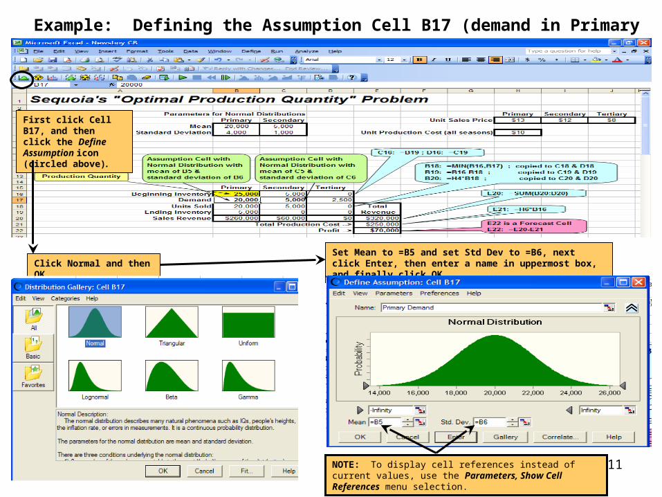
Example: Defining the Assumption Cell B17 (demand in Primary Season)

Click Normal and then OK.Set Mean to =B5 and set Std Dev to =B6, next click Enter, then enter a name in uppermost box, and finally click OK.

First click Cell B17, and then click the Define Assumption icon (circled above).

NOTE: To display cell references instead of current values, use the Parameters, Show Cell References menu selection.

12

Example: Defining the Assumption Cell C17 (demand in Secondary Season)

To Define the Assumption Cell for Cell C17, the demand in the Secondary Season, we could proceed as we just did for Cell B17. However, instead, we will illustrate Crystal Ball’s Copy Data and Paste Data icons.

First click on Cell B17, next click on the Copy Data icon (circled below), then click on Cell C17, and finally click on the Paste Data icon (circled below). To check the copy, click on Cell C17, next click on the Define Assumption icon (circled below), then “proofread” the Mean and Std Dev, then enter a name in the uppermost box, and finally click OK.

13

DefineForecast

Step 3: Define Each Forecast Cell. To define a Forecast Cell, proceed as follows:

After clicking the cell, click the toolbar’s Define Forecast icon to: (1) name the Forecast Cell, and (2) specify the Forecast Cell’s unit of measurement.

14

Example: Defining the Forecast Cell E22 (Profit)

First click Cell E22, and then click the Define Forecast icon (circled below).

Enter the name in the upper box and the units in the lower box, and then click OK. (This step is optional.)

15

Single Step

Step 4: “Debug” the Spreadsheet. Before running the simulation, “debug” the spreadsheet by repeatedly clicking the toolbar’s Single Step icon. Each repetition first generates a new set of sample values for the Assumption Cells and then recalculates the spreadsheet. Careful examination of the successive spreadsheets might reveal an error in the spreadsheet. (NOTE: This is an optional but highly recommended step.)

16

Example: “Debugging” Sequoia’s Spreadsheet

Each click of the Single Step icon (circled below) generates a new set of sample values for the two Assumption Cells (circled below). To “debug” this spreadsheet, continue to click the Single Step icon and “proofread” the resulting numbers until all possible scenarios have occurred: no Ending Inventory after Primary Season, Ending Inventory after Primary Season but no Ending Inventory after Secondary Season, Ending Inventory after both Primary and Secondary Seasons but no Ending Inventory after Tertiary Season, and Ending Inventory after all three seasons.

17

Run Preferences

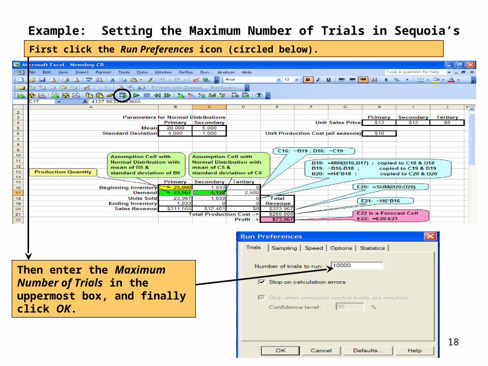
Step 5: Specify the Maximum Number of Trials. To specify the simulation’s maximum number of trails (i.e., iterations or runs), click the toolbar’s Run Preferences icon. In the resulting window, enter the desired number of trials (e.g., 1000, 5000, or 10,000), and then click OK.

18

Example: Setting the Maximum Number of Trials in Sequoia’s Spreadsheet.

Then enter the Maximum Number of Trials in the uppermost box, and finally click OK.

First click the Run Preferences icon (circled below).

19

Start Simulation

Step 6: Run the Simulation. To run the simulation, click the toolbar’s Start Simulation icon.

20

Step 7: View the Simulation’s Results. While the simulation is running and after it ends, Crystal Ball automatically displays in the foreground a window containing a Frequency Chart. (If there are other Forecast Cells, then their corresponding Frequency Charts will be in windows in the background.) The window for a Frequency Chart has its own menu, has a pair of “Certainty Grabbers” along the horizontal axis, and has three “Certainty Boxes” at the bottom. These can be used to perform the following tasks, which are illustrated by the next five slides:

Add to the Frequency Chart a box containing the mean and a corresponding vertical line at the mean value. (This is helpful.)

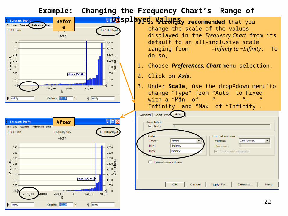
Change the scale of the values displayed in the Frequency Chart from its default to an all-inclusive scale ranging from –Infinity to +Infinity. (This is strongly recommended.)

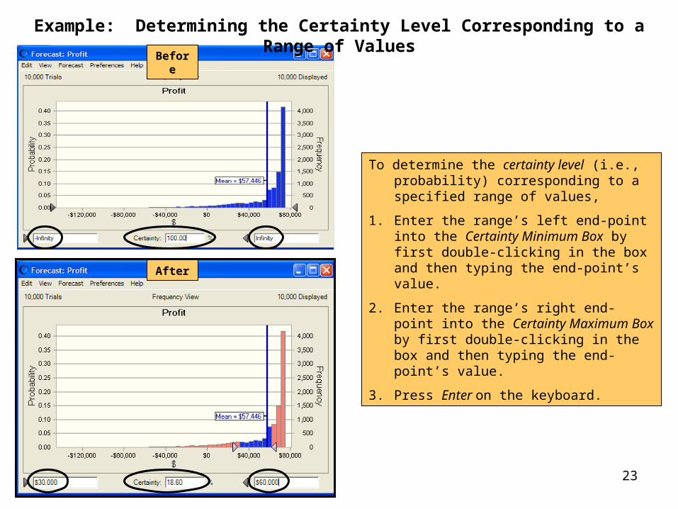
Determine the certainty level (i.e., probability) corresponding to a specified range of values.

Determine a range of values that is located at the chart’s left (right) tail and that corresponds to a specified certainty level.

View summary descriptive statistics

NOTE: If you close the Forecast Charts (by choice or by accident), you can re-open them by clicking the Forecast Charts icon, by clicking the Crystal Ball icon in Excel’s task bar, or by using the Analyze, Forecasts Charts menu selection.

21

Example: Adding the Mean to the Frequency Chart

Before

After

It is helpful to add to the Frequency Chart a box containing the mean and a corresponding vertical line at the mean value. To do so,

1. Choose Preferences, Chart menu selection.

2. Click on Chart Type..

3. Under Marker Lines, check box for “Mean”

22

Before

After

It is strongly recommended that you change the scale of the values displayed in the Frequency Chart from its default to an all-inclusive scale ranging from –Infinity to +Infinity. To do so,

1. Choose Preferences, Chart menu selection.

2. Click on Axis.

3. Under Scale, use the drop-down menu to change “Type” from “Auto” to Fixed” with a “Min” of “–Infinity” and “Max” of “Infinity”.

Example: Changing the Frequency Chart’s Range of Displayed Values

23

Before

After

To determine the certainty level (i.e., probability) corresponding to a specified range of values,

1. Enter the range’s left end-point into the Certainty Minimum Box by first double-clicking in the box and then typing the end-point’s value.

2. Enter the range’s right end-point into the Certainty Maximum Box by first double-clicking in the box and then typing the end-point’s value.

3. Press Enter on the keyboard.

Example: Determining the Certainty Level Corresponding to a Range of Values

24

Before

After

NOTE: Light instead of dark indicates it is “anchored”.

NOTE: Click to “anchor” in place. (Turns from dark to light, as shown below.)

To determine a range of values that is located at the chart’s left (right) tail and that corresponds to a specified certainty level,

1. Click on the left-most (right-most) Certainty Grabber to make it “anchored” (i.e., light-colored instead of dark-colored).

2. Double-click in the Certainty Box, and then type the certainty value (e.g., 10 for 10%) in the Certainty Box,

3. Press Enter on the keyboard.

Example: Determining the “Tail” Value for a Specified Certainty Level

25

After

To view summary descriptive Statistics, choose the View, Statistics menu selection.

To simultaneously view the Frequency Chart and Statistics, choose the View, Split View menu selection.

NOTE

The Mean Standard Error can be used to construct a confidence interval for the Mean. As examples, the 95% confidence interval for containing the true mean is

$57,446 ± (1.645)($251),and the 97.5% confidence interval is

$57,446 ± (1.96)($251).The more trials, the lower the Mean Standard Error, and the tighter the confidence interval.

$25110,000

$25,083

n

σErrorStandardMean

Example: Viewing Summary Statistics

26Create Report

Step 8: Save and Print the Simulation’s Results. Crystal Ball can create a summary report in the form of a spreadsheet that can be modified, printed, or saved in the same manner as any other spreadsheet. To do so, first click the toolbar’s Create Report icon (or choose the Analyze, Create Report menu selection). Then, using the resulting dialog box, customize the report. Although you may experiment with other preferences, see the next slide for my recommended preferences for “beginners”.

NOTES: To have Crystal Ball place the report in a new worksheet in current workbook, be sure to proceed as illustrated on the next slide. If you don’t do this, the Report will be placed in a worksheet in a new workbook. To move the worksheet to the current workbook, use Excel’s Edit, Move or Copy Sheet menu selection.

To add gridlines and/or row and column headings to the Report, choose Excel’s Tools, Options, View menu selection.

27

To create the “plain vanilla” summary report contained in the spreadsheet on the next slide,

1. Click the Create Report icon.2. At the top of the “Create Report Preferences” window, click

Options, and then, to create the report as a new worksheet in the current workbook, click the Current Workbook radio button.

3. At the top of the “Create Report Preferences” window, click Reports.

4. Click on “Custom” in the lower-right.5. In the “Custom Report” window, in “Report Sections” and

“Forecast Details”, click the boxes indicated below.6. Click OK twice to create the report on the next slide.

Example: Saving and Printing the Simulation’s Results

28

NOTE: To add gridlines and/or row and column headings to the Report, choose Excel’s Tools, Options, View menu selection.

Example: Saving and Printing the Simulation’s Results (continued)

NOTE: The report displays the Frequency Chart in its format at the time the Create Report icon was clicked.

29DefineAssumption

DefineForecast

Copy Data Paste Data Run Preferences

Start Simulation Single Step Create Report

Summary of Steps for Running a Simulation Using Crystal Ball

1. Construct the Spreadsheet.2. Define Each Assumption Cell.3. Define Each Forecast Cell.4. “Debug” the Spreadsheet.5. Specify the Maximum Number of Trials.6. Run the Simulation.7. View the Simulation’s Results.8. Save and Print the Simulation’s Results.

3

5

46 8

2

Use when some Assumption Cells have a common distribution, perhaps with different parameters.

2

30

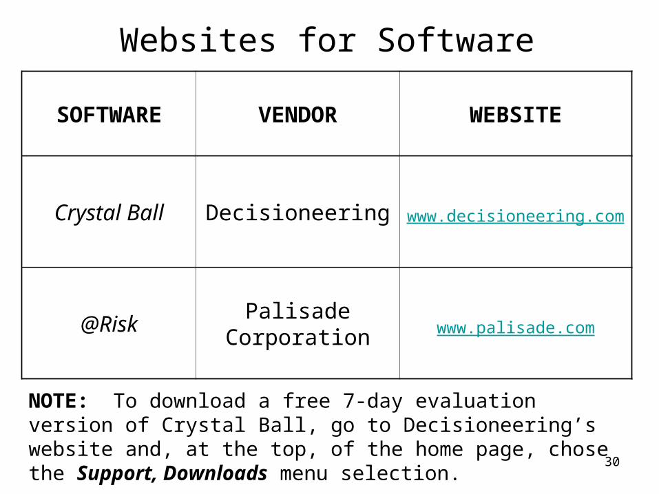
Websites for Software

SOFTWARE VENDOR WEBSITE

Crystal Ball Decisioneering www.decisioneering.com

@RiskPalisade

Corporation www.palisade.com

NOTE: To download a free 7-day evaluation version of Crystal Ball, go to Decisioneering’s website and, at the top, of the home page, chose the Support, Downloads menu selection.

31

An Introduction toRisk Management

(using Sequoia’s Optimal Production Quantity Problem)

For this portion of the session, the learning objectives are:

Learn the meaning of Risk and the meaning of Risk Management.

Learn the distinction between a good decision and a good outcome.

Understand scenarios where it is not appropriate to maximize Expected Monetary Value.

Learn decision-making criteria that take risk into account and that are alternatives to maximizing Expected Monetary Value.

32

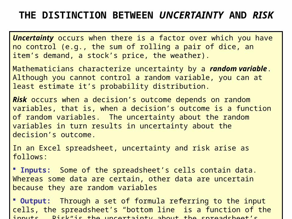
Uncertainty occurs when there is a factor over which you have no control (e.g., the sum of rolling a pair of dice, an item’s demand, a stock’s price, the weather).

Mathematicians characterize uncertainty by a random variable. Although you cannot control a random variable, you can at least estimate it’s probability distribution.

Risk occurs when a decision’s outcome depends on random variables, that is, when a decision’s outcome is a function of random variables. The uncertainty about the random variables in turn results in uncertainty about the decision’s outcome.

In an Excel spreadsheet, uncertainty and risk arise as follows:

Inputs: Some of the spreadsheet’s cells contain data. Whereas some data are certain, other data are uncertain because they are random variables

Output: Through a set of formula referring to the input cells, the spreadsheet’s “bottom line” is a function of the inputs. Risk is the uncertainty about the spreadsheet’s “bottom line” that results from the uncertainty about (at least some of) the spreadsheet’s inputs.

THE DISTINCTION BETWEEN UNCERTAINTY AND RISK

33

Although risk cannot be controlled, it can at least be “managed”.

In this session, you will learn about Risk Management -- a logical framework for making a decision when the decision has an uncertain outcome.

DEFINITION OF RISK MANAGEMENT

34

Risk Management grew from “roots” established during the Renaissance, when scientific and mathematical discoveries motivated challenges to long-held beliefs and facilitated unprecedented innovation and exploration.

During the middle of the 17-th century, two French mathematicians -- Blaise Pascal and Pierre de Fermat – “discovered” the theory of probability, the foundation of Risk Management.

In addition to being a mathematician, Pascal was a religious philosopher and is often credited with making the first statement about Risk Management. In handwritten notes known as “Pascal’s Wager”, Pascal analyzed the future consequences of believing or not believing in the existence of God. Pascal concluded that one should believe in God because, to paraphrase Pascal,

If you believe in God and there is none, then "no big deal". But, if you do not believe in God and there is one, then "BIG DEAL"!

In the 17-th century, Dutch farmers bought options on the price of tulips.

HISTORY OF RISK MANAGEMENT

35

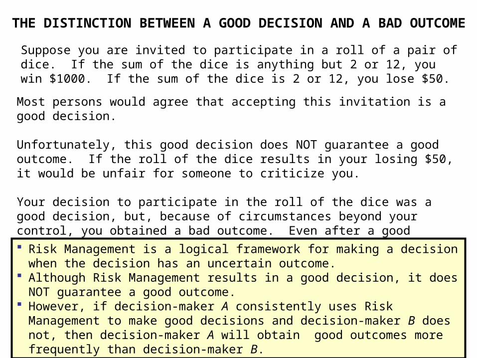
Most persons would agree that accepting this invitation is a good decision.

Unfortunately, this good decision does NOT guarantee a good outcome. If the roll of the dice results in your losing $50, it would be unfair for someone to criticize you.

Your decision to participate in the roll of the dice was a good decision, but, because of circumstances beyond your control, you obtained a bad outcome. Even after a good decision has been made, "luck" (that is, uncertainty) will play a role in determining whether the good decision results in a good or bad outcome.

Risk Management is a logical framework for making a decision when the decision has an uncertain outcome.

Although Risk Management results in a good decision, it does NOT guarantee a good outcome.

However, if decision-maker A consistently uses Risk Management to make good decisions and decision-maker B does not, then decision-maker A will obtain good outcomes more frequently than decision-maker B.

THE DISTINCTION BETWEEN A GOOD DECISION AND A BAD OUTCOME

Suppose you are invited to participate in a roll of a pair of dice. If the sum of the dice is anything but 2 or 12, you win $1000. If the sum of the dice is 2 or 12, you lose $50.

36

Motivation for the Return-Risk-Ratio

The Return-to-Risk Ratio is the ratio of the Mean to the Standard Deviation.

In the tables below, which scenario would you choose – A or B?

PROFIT Scenario A Scenario B

Mean 100 50 Std. Dev. 25 25

Ratio 4 2

PROFIT Scenario A Scenario B

Mean 100 100 Std. Dev. 50 20

Ratio 2 5

PROFIT Scenario A Scenario B

Mean 100 50 Std. Dev. 25 10

Ratio 4 5

PROFIT Scenario A Scenario B

Mean 150 50 Std. Dev. 25 10

Ratio 6 5

In Tables 1 & 2, it is clear that you should choose the scenario with the higher Return-to-Risk Ratio. Some decision-makers argue that this should also be true for Tables 3 & 4.

Note that, as the Mean increases (which is good) and the Standard Deviation decreases (which is good for someone who is risk-averse), then the Return-to-Risk Ratio increases. This is the motivation for maximizing the Return-to-Risk Ratio.

37

EXAMPLE OF RISK MANAGEMENTAn investment’s revenue is estimated to be one of six equally-likely values:

$1, $2, $3, $4, $5, or $6.

Think of the revenue as being determined by the roll of a die.

The investment costs $2.5, but, when 2 investments are purchased, there is a supplemental transaction charge of $0.1.

The table below analyzes two alternatives:

Alternative #1: You own 100% of 1 investment.

Alternative #2: You own 50% of 2 identical but independent investments.

1/6 1/6 1/6 1/6 1/6 1/6 6/365/36 4&3 5/36

4/36 3&3 3&4 4&4 4/363/36 3&2 4&2 5&2 5&3 5&4 3/36

2/36 2&2 2&3 2&4 2&5 3&5 4&5 5&5 2/361/36 2&1 3&1 4&1 5&1 6&1 6&2 6&3 6&4 6&5 1/361&1 1&2 1&3 1&4 1&5 1&6 2&6 3&6 4&6 5&6 6&6

DIE | AVERAGE OF DICE 1 2 3 4 5 6 1 1.5 2 2.5 3 3.5 4 4.5 5 5.5 6PAYOFF (1.5) (0.5) 0.5 1.5 2.5 3.5 (1.6) (1.1) (0.6) (0.1) 0.4 0.9 1.4 1.9 2.4 2.9 3.4

LOSS (if any) 1.5 0.5 0.0 0.0 0.0 0.0 1.6 1.1 0.6 0.1 0.0 0.0 0.0 0.0 0.0 0.0 0.0

ALTERNATIVE #1OWN 100% OF 1 INVESTMENT

ALTERNATIVE #2

PAYOFF = DIE - 2.5

OWN 50% OF 2 IDENTICAL BUT INDEPENDENT INVESTMENTS(For 2 investments, there is a supplemental transaction charge of $0.1.)

PAYOFF = (.5)(DIE #1 - 2.5) + (.5)(DIE #2 - 2.5) -0.1 = AVERAGE OF DICE - 2.6

38

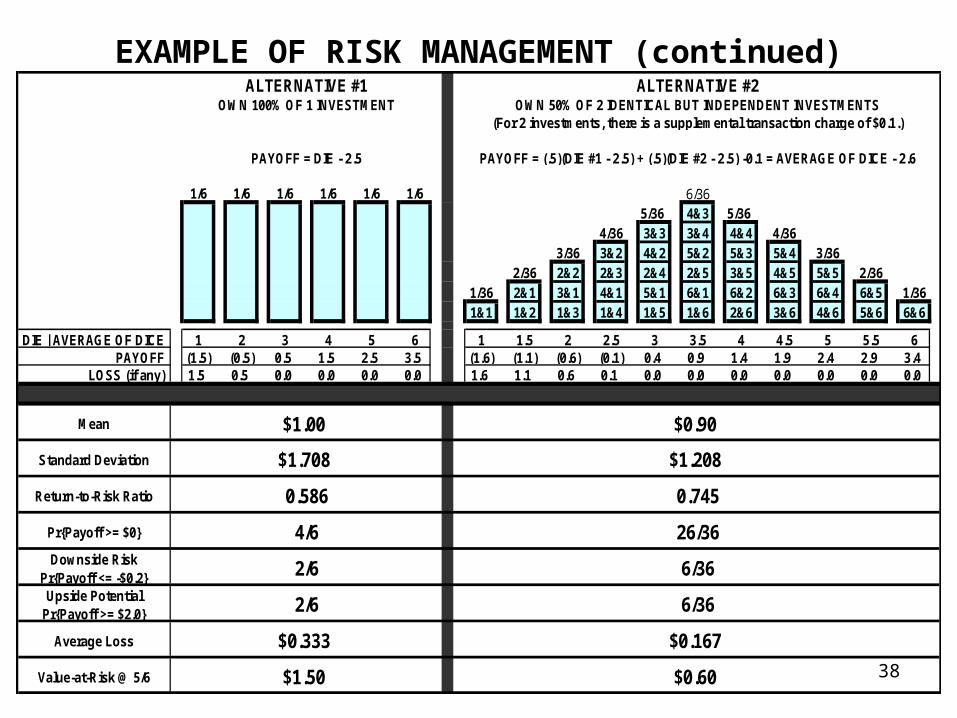
EXAMPLE OF RISK MANAGEMENT (continued)

1/6 1/6 1/6 1/6 1/6 1/6 6/365/36 4&3 5/36

4/36 3&3 3&4 4&4 4/363/36 3&2 4&2 5&2 5&3 5&4 3/36

2/36 2&2 2&3 2&4 2&5 3&5 4&5 5&5 2/361/36 2&1 3&1 4&1 5&1 6&1 6&2 6&3 6&4 6&5 1/361&1 1&2 1&3 1&4 1&5 1&6 2&6 3&6 4&6 5&6 6&6

DIE | AVERAGE OF DICE 1 2 3 4 5 6 1 1.5 2 2.5 3 3.5 4 4.5 5 5.5 6PAYOFF (1.5) (0.5) 0.5 1.5 2.5 3.5 (1.6) (1.1) (0.6) (0.1) 0.4 0.9 1.4 1.9 2.4 2.9 3.4

LOSS (if any) 1.5 0.5 0.0 0.0 0.0 0.0 1.6 1.1 0.6 0.1 0.0 0.0 0.0 0.0 0.0 0.0 0.0

Mean

Standard Deviation

Return-to-Risk Ratio

Pr{Payoff >= $0}

Downside RiskPr{Payoff <= -$0.2}Upside Potential

Pr{Payoff >= $2.0}

Average Loss

Value-at-Risk @ 5/6

ALTERNATIVE #1OWN 100% OF 1 INVESTMENT

ALTERNATIVE #2

PAYOFF = DIE - 2.5

OWN 50% OF 2 IDENTICAL BUT INDEPENDENT INVESTMENTS(For 2 investments, there is a supplemental transaction charge of $0.1.)

PAYOFF = (.5)(DIE #1 - 2.5) + (.5)(DIE #2 - 2.5) -0.1 = AVERAGE OF DICE - 2.6

$1.00

$1.708

0.586

4/6

2/6

2/6

$0.333

$1.50

$0.90

$1.208

0.745

26/36

6/36

6/36

$0.167

$0.60

39

Maximizing the Expected Monetary Value is appropriate when the decision-maker will encounter the same situation a very large number of times and can afford to "play the averages" (that is, can survive large losses or widely varying payoffs, as long as the average payoff is maximized).

However, maximizing the Expected Monetary Value is not appropriate when the decision-maker will encounter the situation only once and is risk-averse or risk-seeking, when a large loss would be catastrophic, and/or when the payoff’s standard deviation is important.

WHEN MAXIMIZING EXPECTED MONETARY VALUE (EMV)

IS NOT APPROPRIATE

40

ALTERNATIVE DECISION-MAKING CRITERIA IN THE CONTEXT OF

SEQUOIA’S OPTIMAL PRODUCTION QUANTITY PROBLEM

In our previous consideration of Sequoia’s Optimal Production Quantity Problem, we analyzed only the case where the production quantity was 25,000 units.

Now, we want to consider five alternative production quantities:

17,500 , 20,000 , 22,500 , 25,000, & 27,500.

We want to compare these five alternatives across the 8 alternative decision-making criteria summarized in the table on the next slide:

41

To fill-in the above table, we simply run our simulation five times, each time with a different value for the Production Quantity in Cell B16.

NOTE: It would be more efficient to use Crystal Ball’s Decision Table Tool, but we will postpone our discussion of this tool until a future session.

PRODUCTION QUANTITY (Q ) PROFIT (P ) 17,500 20,000 22,500 25,000 27,500 Criterion for "Optimal"

Mean <-- Maximize Mean.

Standard Deviation <-- Minimize Standard Deviation.

Return-to-Risk Ratio <-- Maximize Risk-to-Return Ratio.Pr{P >= $0} <-- Maximize Pr{P >= $0}.

Worst Case <-- Maximize Worst Case.Downside Risk defined as Pr{P <= $25,000} <-- Minimize Downside Risk.

Best Case <-- Maximize Best Case.Upside Potential defined as Pr{P >= $50,000} <-- Maximize Upside Potential.

42

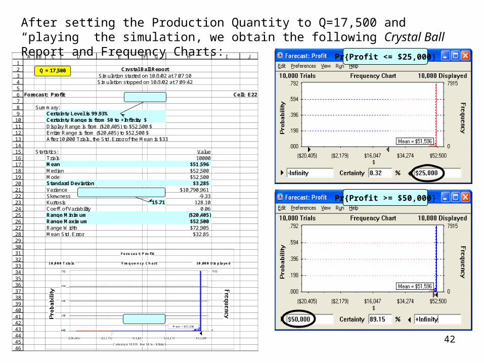
After setting the Production Quantity to Q=17,500 and “playing” the simulation, we obtain the following Crystal Ball Report and Frequency Charts:

Pr{Profit <= $25,000}

Pr{Profit >= $50,000}

12345678910111213141516171819202122232425262728293031323334353637383940414243444546

A B C D E F G H I J

Crystal Ball ReportSimulation started on 10/3/02 at 7:07:10Simulation stopped on 10/3/02 at 7:09:42

Forecast: Profit Cell: E22

Summary:Certainty Level is 99.93%Certainty Range is from $0 to +Infinity $Display Range is from ($20,405) to $52,500 $Entire Range is from ($20,405) to $52,500 $After 10,000 Trials, the Std. Error of the Mean is $33

Statistics: ValueTrials 10000Mean $51,596Median $52,500Mode $52,500Standard Deviation $3,285Variance $10,790,961Skewness -9.33Kurtosis 15.71 128.10Coeff. of Variability 0.06Range Minimum ($20,405)Range Maximum $52,500Range Width $72,905Mean Std. Error $32.85

Frequency Chart

Certainty is 99.93% from $0 to +Infinity $

Mean = $51,596.000

.198

.396

.594

.792

0

7915

($20,405) ($2,179) $16,047 $34,274 $52,500

10,000 Trials 10,000 Displayed

Forecas t: Profit

Q = 17,500

Pr{Profit >= 0}

Return-to-Risk Ratio = H17/H20

Pr{Profit >= 0}

43

After running our simulation five times – each time with a different value for the Production Quantity – we obtain the following table:

So, given the above table, what advice would we give to Sequoia?

PRODUCTION QUANTITY (Q ) PROFIT (P ) 17,500 20,000 22,500 25,000 27,500 Criterion for "Optimal"

Mean $51,596 $57,152 $59,798 $57,657 $49,176 <-- Maximize Mean.

Standard Deviation $3,285 $7,817 $15,414 $25,067 $35,329 <-- Minimize Standard Deviation.

Return-to-Risk Ratio 15.71 7.31 3.88 2.30 1.39 <-- Maximize Risk-to-Return Ratio.Pr{P >= $0} 0.9993 0.9974 0.9829 0.9533 0.8863 <-- Maximize Pr{P >= $0}.

Worst Case ($20,405) ($82,805) ($117,239) ($138,679) ($166,499) <-- Maximize Worst Case.Downside Risk defined as Pr{P <= $25,000} 0.0032 0.0161 0.0463 0.1114 0.2231 <-- Minimize Downside Risk.

Best Case $52,500 $60,000 $67,500 $75,000 $82,500 <-- Maximize Best Case.Upside Potential defined as Pr{P >= $50,000} 0.8915 0.9326 0.8870 0.7742 0.6131 <-- Maximize Upside Potential.

44

SUMMARY OF ALTERNATIVE DECISION-MAKING CRITERIA

1. Maximize the Mean of Profit (that is, the Expected Value of Profit).

2. Minimize the Standard Deviation of Profit, subject to a constraint that the Mean of Profit is greater than or equal to some specified “target value”.

3. Maximize the Return-to-Risk Ratio, that is, maximize the ratio of the Mean to the Standard Deviation. (Note: The Return-to-Risk Ratio equals the inverse of the Coefficient of Variability.)

4. Assuming that Profit can be negative (that is, that there can be a loss), then maximize the probability of a nonnegative profit (that is, the probability that there will NOT be a loss).

6. Minimize Downside Risk (that is, the probability that Profit is <= a specified low value).

8. Maximize Upside Potential (that is, the probability that Profit is >= a specified high value).

9. Between two decisions, choose the decision that has the higher probability of outperforming the other decision. (NOTE: We will postpone our discussion of this criterion until a future session.)

10. Assuming that Profit can be negative (that is, that there can be a loss), then minimize the Value-at-Risk (VaR) for a specified confidence interval such as 95% (that is, minimize the loss value which will be exceeded only 5% of the time). (NOTE: We will postpone our discussion of this criterion until a future session.)

NOTE: Instead of maximizing profit, we might be maximizing something else, such as Net Present Value.

5. Maximize the Worst Case.

7. Maximize the Best Case.