1

Scatter Component Analysis: A Unified Frameworkfor Domain Adaptation and Domain Generalization

Muhammad Ghifary, David Balduzzi, W. Bastiaan Kleijn, and Mengjie ZhangVictoria University of Wellington

{muhammad.ghifary,bastiaan.kleijn,mengjie.zhang}@ecs.vuw.ac.nz, david.balduzzi@vuw.ac.nz

Abstract—This paper addresses classification tasks on a particular target domain in which labeled training data are only available fromsource domains different from (but related to) the target. Two closely related frameworks, domain adaptation and domain generalization, areconcerned with such tasks, where the only difference between those frameworks is the availability of the unlabeled target data: domainadaptation can leverage unlabeled target information, while domain generalization cannot. We propose Scatter Component Analyis (SCA), afast representation learning algorithm that can be applied to both domain adaptation and domain generalization. SCA is based on a simplegeometrical measure, i.e., scatter, which operates on reproducing kernel Hilbert space. SCA finds a representation that trades betweenmaximizing the separability of classes, minimizing the mismatch between domains, and maximizing the separability of data; each of which isquantified through scatter. The optimization problem of SCA can be reduced to a generalized eigenvalue problem, which results in a fast andexact solution. Comprehensive experiments on benchmark cross-domain object recognition datasets verify that SCA performs much fasterthan several state-of-the-art algorithms and also provides state-of-the-art classification accuracy in both domain adaptation and domaingeneralization. We also show that scatter can be used to establish a theoretical generalization bound in the case of domain adaptation.

Index Terms—Domain adaptation, domain generalization, feature learning, kernel methods, scatter, object recognition.

F

1 INTRODUCTION

Supervised learning is perhaps the most popular task in machinelearning and has recently achieved dramatic successes in manyapplications such as object recognition [1], [2], object detection [3],speech recognition [4], and machine translation [5]. These successesderive in large part from the availability of massive labeled datasetssuch as PASCAL VOC2007 [6] and ImageNet [7]. Unfortunately,obtaining labels is often a time-consuming and costly process thatrequires human experts. Furthermore, the process of collecting sam-ples is prone to dataset bias [8], [9], i.e., a learning algorithmtrained on a particular dataset generalizes poorly across datasets. Inobject recognition, for example, training images may be collectedunder specific conditions involving camera viewpoints, backgrounds,lighting conditions, and object transformations. In such situations, theclassifiers obtained with learning algorithms operating on samplesfrom one dataset cannot be directly applied to other related datasets.Developing learning algorithms that are robust to label scarcity anddataset bias is therefore an important and compelling problem.

Domain adaptation [10] and domain generalization [11] havebeen proposed to overcome the fore-mentioned issues. In this context,a domain represents a probability distribution from which the samplesare drawn and is often equated with a dataset. The domain isusually divided into two different types: the source domain andthe target domain, to distinguish between a domain with labeledsamples and a domain without labeled samples. These two domainsare related but different, which limits the applicability of standardsupervised learning models on the target domain. In particular, thebasic assumption in standard supervised learning that training andtest data come from the same distribution is violated.

The goal of domain adaptation is to produce good models ona target domain, by training on labels from the source domain(s)and leveraging unlabeled samples from the target domain as supple-mentary information during training. Domain adaptation has demon-strated significant successes in various applications, such as sentiment

classification [12], [13], [14], visual object recognition [15], [16],[17], [18], and WiFi localization [19].

Finally, the problem of domain generalization arises in situationswhere unlabeled target samples are not available, but samples frommultiple source domains can be accessed. Examples of domain gen-eralization applications are automatic gating of flow cytometry [11],[20] and visual object recognition [21], [22], [23].

The main practical issue is that several state-of-the-art domainadaptation and domain generalization algorithms for object recogni-tion result in optimization problems that are inefficient to solve [16],[18], [23], [24]. Therefore, they may not be suitable in situationsthat require a real-time learning stage. Furthermore, although domainadaptation and domain generalization are closely related problems,domain adaptation algorithms cannot in general be applied directlyto domain generalization, since they rely on the availability of(unlabeled) samples from the target domain. It is highly desirableto develop algorithms that can be computed more efficiently, arecompatible with both domain adaptation and domain generalization,and provides state-of-the-art performance.

1.1 Goals and Objectives

To address the fore-mentioned issues, we propose a fast unifiedalgorithm for reducing dataset bias that can be used for both domainadaptation and domain generalization. The basic idea of our algorithmis to learn representations as inputs to a classifier that are invariant todataset bias. Intuitively, the learnt representations should incorporatefour requirements: (i) separate points with different labels and (ii)separate the data as a whole (high variance), whilst (iii) not separatingpoints sharing a label and (iv) not separating the two or more domains.The main contributions of this paper are as follows:

• The first contribution is scatter, a simple geometric functionthat quantifies the mean squared distance of a distributionfrom its centroid. We show that the above four requirements

arX

iv:1

510.

0437

3v1

[cs

.CV

] 1

5 O

ct 2

015

2

can be encoded through scatter and establish the relationshipwith Linear Discriminant Analysis [25], Principal ComponentAnalysis, Maximum Mean Discrepancy [26] and Distribu-tional Variance [20].

• The second contribution is a fast scatter-based feature learn-ing algorithm that can be applied to both domain adapta-tion and domain generalization problems, Scatter ComponentAnalysis (SCA). The optimization reduces to a generalizedeigenproblem that admits a fast and exact solution on parwith Kernel PCA [27] in terms of time complexity.

• The third contribution is the derivation of a theoretical boundfor SCA in the case of domain adaptation. Our theoreticalanalysis shows that domain scatter controls the general-ization performance of SCA. Under certain circumstances,we demonstrate that domain scatter has a connection withdiscrepancy distance, which has previously been shown tocontrol the generalization performance of domain adaptationalgorithms [28].

We performed extensive experiments to evaluate the performanceof SCA against a large suite of alternatives. We found that SCAperforms considerably faster than the prior state-of-the-art across arange of visual object cross-domain recognition, with competitive orbetter performance in terms of accuracy.

1.2 Organization of the PaperThis paper is organized as follows. Section 2 describes the problemdefinitions and reviews existing work on domain adaptation anddomain generalization. Sections 3 and 4 describes our proposedtool and also the corresponding feature learning algorithm, ScatterComponent Analysis (SCA). The theoretical domain adaptation boundfor SCA is then presented in Section 5. Comprehensive evaluationresults and analyses are provided in Sections 6 and 7. Finally, Section8 concludes the paper.

2 BACKGROUND AND LITERATURE REVIEW

This section establishes the basic definitions of domains, domainadaptation, and domain generalization. It then reviews existing workin domain adaptation and domain generalization, particularly in thearea of computer vision and object recognition.

A domain is a probability distribution PXY on X × Y , whereX and Y are the input and label spaces respectively. For thesake of simplicity, we equate PXY with P. The terms domainand distribution are used interchangeably throughout the paper. LetS = {xi, yi}ni=1 ∼ P be an i.i.d. sample from a domain. It isconvenient to use the notation P for the corresponding empiricaldistribution P(x, y) = 1

n

∑ni=1 δ(xi,yi)(x, y), where δ is the Dirac

delta.We define domain adaptation and domain generalization as

follows.

Definition 1 (Domain Adaptation). Let Ps and Pt be a sourceand target domain respectively, where Ps 6= Pt. Denote by Ss ={xsi , ysi }

nsi=1 ∼ Ps and Stu = {xti}

nti=1 ∼ PtX samples drawn from

both domains. The task of domain adaptation is to learn a goodlabeling function fPt : X → Y given Ss and Stu as the trainingexamples.

Definition 2 (Domain Generalization). Let ∆ = {P1, . . . ,Pm} bea set of m source domains and Pt /∈ ∆ be a target domain. Denoteby Sd = {xdi , ydi }

ndi=1 ∼ Pd samples drawn from m source domains.

The task of domain generalization is to learn a labeling functionfPt : X → Y given Sd,∀d = 1, ...,m as the training examples.

It is instructive to compare these two related definitions. The maindifference between domain adaptation and domain generalization ison the availability of the unlabeled target samples. Both have thesame goal: learning a labeling function f : X → Y that performswell on the target domain. In practice, domain generalization requiresm > 1 to work well although m = 1 might not violate Definition 2.Note that domain generalization can be exactly reduced to domainadaptation if m = 2 and PtX ∈ ∆.

Domain adaptation and domain generalization have recently at-tracted great interest in machine learning. We present a review ofrecent literature that is organized into two parts: i) domain adaptationand ii) domain generalization.

2.1 Domain AdaptationEarlier studies on domain adaptation focused on natural languageprocessing, see, e.g., [29] and references therein. A notable algorithmin this area is Structural Correspondence Learning (SCL) [10]. SCLuses unlabeled data from both source and target domains to modelcorrespondences among features with pivot features, that is, thosethat occur frequently and behave similarly in both domains. The pivotfeatures are then used to learn a mapping from the original featurespace to a shared, transformed feature space in which the domaindifference is reduced.

Recently, a number of domain adaptation works have been con-cerned with computer vision and object recognition [17], [30], [31],[32], [33], [34]. The reader is encouraged to consult the recent surveyin visual domain adaptation [35] for a more comprehensive review.We classify domain adaptation algorithms into three categories: i) theclassifier adaptation approach, ii) the selection/reweighting approach,and iii) the feature transformation-based approach.

The classifier adaptation approach aims to learn a good, adap-tive classifier on a target domain by leveraging knowledge fromsource or auxiliary domains. Adaptive Support Vector Machines (A-SVMs) [36] utilize auxiliary classifiers to adapt a primary classifierthat performs well on a target domain, where the optimizationcriterion is similar to standard SVMs. Domain Adaptation Machine(DAM) [37] employs both Laplacian manifold (to make use ofunlabeled target data) and sparsity regularizations in Least-SquaresSVMs [38]. A-SVMs and DAM are examples of successful applica-tions in video concept detection.

The reweighting/selection approach reduces sample bias byreweighting or selecting source instances that are ‘close’ to targetinstances – Selection can be considered as the ‘hard’ version ofreweighting. The basic idea has been studied under the name ofcovariate shift [39]. Gong et al. [40] applied a convex optimizationstrategy to select some source images that are maximally similar tothe target images according to Maximum Mean Discrepancy [41] –referred to as landmarks. The landmarks are then used to constructmultiple auxiliary tasks as a basis for composing domain-invariantfeatures. Transfer Joint Matching (TJM) [16] uses a reweightingstrategy as a regularizer based on `2,1-norm structured sparsity onthe source subspace bases.

The feature transformation-based approach is perhaps the mostpopular approach in domain adaptation. Here the notion of transfor-mation has a broad meaning: feature projection, alignment, augmen-tation, etc. A kernelized projection-based algorithm, Transfer Com-ponent Analysis (TCA) and its semi-supervised version SSTCA [42],utilizes Maximum Mean Discrepancy (MMD) [41] to extract domain-invariant features for WiFi localization and text classification. Somemetric learning-based methods have been proposed, which can beconsidered as early works on the Office cross-domain recogni-tion [17], [43]. The idea of finding ‘intermediate features’ by exploit-

3

ing geodesic distances on Grassmann manifolds, where a point on themanifold is an orthogonal subspace, was also considered [30], [44].These ‘intermediate features’ can also be constructed by probablya simpler approach: aligning two different subspaces by a linearoperator [32]. Algorithms based on hierarchical non-linear feature ordeep learning are also capable of producing powerful domain adaptivefeatures [15], [45], [46], [47], [48], [49]. The algorithm proposed inthis paper belongs to the feature transformation-based approach.

Some works have addressed Probably Approximately Correct(PAC) theoretical bounds for domain adaptation. Ben-David et al. [50]presented the first theoretical analysis of domain adaptation, that is,an adaptation generalization bound in classification tasks based on thedA-distance. Mansour et al. [28] extended this work in several waysbuilt on Rademacher complexity [51] and the discrepancy distance,as an alternative to dA-distance. In this paper, we provide a domainadaptation bound for our new algorithm based on the latter analysis.

2.2 Domain GeneralizationDomain generalization is a newer line of research than domainadaptation. Blanchard et al. [11] first studied this issue and proposedan augmented SVM that encodes empirical marginal distributions intothe kernel for solving automatic gating of flow cytometry. A featureprojection-based algorithm, Domain-Invariant Component Analysis(DICA) [20], was then introduced to solve the same problem.DICA extends Kernel PCA [27] by incorporating the distributionalvariance to reduce the dissimilarity across domains and the centralsubspace [52] to capture the functional relationship between thefeatures and their corresponding labels.

Domain generalization algorithms also have been used in objectrecognition. Khosla et al. [22] proposed a multi-task max-marginclassifier, which we refer to as Undo-Bias, that explicitly encodesdataset-specific biases in feature space. These biases are used topush the dataset-specific weights to be similar to the global weights.Fang et al. [21] developed Unbiased Metric Learning (UML) basedon a learning-to-rank framework. Validated on weakly-labeled webimages, UML produces a less biased distance metric that providesgood object recognition performance. More recently, Xu et al. [23]extended an exemplar-SVM [53] to domain generalization by addinga nuclear norm-based regularizer that captures the likelihoods of allpositive samples. The proposed model is referred to as LRE-SVM.

Although both domain adaptation and domain generalization havethe same goal (reducing dataset bias), the approaches are generallynot compatible to each other – domain adaptation methods cannotbe directly applied to domain generalization or vice versa. To ourbest knowledge, only LRE-SVM has this compatibility. Furthermore,several state-of-the-art domain adaptation and domain generalizationalgorithms, including LRE-SVM, require the solution of a computa-tionally complex optimization that induces high complexity in time.In this work, we establish a fast algorithm that overcomes the aboveissues.

3 SCATTER

We work in a feature space that is a reproducing kernel Hilbert space(RKHS) H. The main motivation is to transform original inputs ontoH, which is high or possibly infinite dimensional space, with thehope that the new features are linearly separable. The most importantproperty of RKHS is perhaps to allow a computationally feasibletransformation onto H by virtue of the kernel trick.

Definition 3 (Reproducing Kernel Hilbert Space). Let X bean arbitrary set and H ⊂ {f : X → R} a Hilbert space offunctions on X . Define the evaluation functional Lx : H → R by

Lx[h] := h(x),∀h ∈ H. Then H is a reproducing kernel Hilbertspace (RKHS) if the functional Lx is always bounded: i.e. for allx ∈ X there exists an λx > 0 such that

|Lx[h]| = |h(x)| ≤ λx‖h‖H. (1)

It follows that there is a function φ : X → H (referred to as thecanonical feature map) satisfying:

Lx[h] = 〈h, φ(x)〉 = h(x) for all h ∈ H and x ∈ X . (2)

Consequently, for each t ∈ X , one can write

〈φ(t), φ(x)〉 =: κ(t, x).

The function κ : X × X → R is referred to as the reproducingkernel.

Expression (1) is the weakest condition that ensures the existenceof an inner product and also the ability to evaluate each function inHat every point in the domain, while (2) provides more useful notionin practice.

Before introducing scatter, it is convenient to first representdomains as points in RKHS using the mean map [54]:

Definition 4 (Mean map). Suppose that X is equipped with a kernel,and thatH is the corresponding RKHS with feature map φ : X → H.Let ∆X denote the set of probability distributions on X . The meanmap takes distributions on X to points in H:

µ : ∆X → H : P 7→ Ex∼P

[φ(x)

]=: µP.

Geometrically, the mean map is the centroid of the image of thedistribution under φ. We define scatter as the variance of points inthe image around its centroid:

Definition 5 (Scatter). The scatter of distribution P on X relative toφ is

Ψφ(P) := Ex∼P

[∥∥µP − φ(x)∥∥2H

]where ‖ · ‖H is the norm on H.

The scatter of a domain cannot be computed directly; instead it isestimated from observations. The scatter of a finite set of observations{x1, . . . , xn} is computed with respect to the empirical distribution

P(x) :=1

n

n∑i=1

δxi(x) where δxi

(x) =

{1 if xi = x

0 else.

We provide a theorem that shows how the difference between thetrue scatter and a finite sample estimate decreases with the samplesize. To do so, we need a concentration of measure bound referred toas McDiarmid’s inequality [55].

Theorem 1 (McDiarmid’s Inequality). Let X1, ..., Xn be indepen-dent random variables taking values in the set X under a distributionP. Further, let f : Xn → R be a function of X1, .., Xn that satisfies

supx1...xn,x′i∈X

∣∣f(x1 . . . xi . . . xn)− f(x1 . . . x′i . . . xn)

∣∣ ≤ ci,where xi 6= x′i and 1 ≤ i ≤ n. The following inequality holds for allε > 0

P{∣∣E[f ]− f

∣∣ ≥ ε} ≤ 2 exp

( −2ε2∑ni=1 c

2i

).

Now it is convenient to bound the difference between the empiri-cal scatter and the true scatter given by the following theorem:

Theorem 2 (Scatter Bound). Suppose P is a true distribution overall samples of size n and P is its empirical distribution. Further

4

suppose that ‖φ(x)‖2 ≤ M for all x ∈ X . Then, with probability≥ 1− δ, ∣∣Ψφ(P)−Ψφ(P)

∣∣ ≤M√

2 log( 2δ )

n.

Proof. Let Ψi←x := Ψφ(x1 . . . xi−1, x, xi+1 . . . xn). It is easy tosee that

supx1...xn,x∈X

|Ψφ(x1 . . . xn)−Ψi←x(x1 . . . xn)| ≤ 2M

n

for all i. By Theorem 1 we get

P{∣∣Ψφ(P)−Ψφ(P)

∣∣ > ε}≤ 2 exp

(−ε

2 · n2M2

).

By setting δ = 2 exp(− ε2·n

2M2

), the results follows directly.

We provide an example for later use. If the input space is a vectorspace and φ is the identity then it follows immediately that

Lemma 3 (Total variance as scatter). The scatter of the set of d-dimensional points (in a matrix form) X = [x1, . . . ,xn]> ∈ Rn×drelative to the identity map φ : Rd → Rd, i.e., φ(x) := x, is thetotal variance:

Ψ(X) = Tr(X− X)>(X− X) = Tr Cov(X),

where Tr(·) denotes the trace operation and X = [x, . . . , x]> withx =

∑ni=1 xi.

We utilize scatter to formulate a feature learning algorithmreferred to as Scatter Component Analysis (SCA). Specifically, scat-ter quantifies requirements needed in SCA to develop an effectivesolution for both domain adaptation and generalization, which willbe described in the next section.

4 SCATTER COMPONENT ANALYSIS (SCA)SCA aims to efficiently learn a representation that improves bothdomain adaptation and domain generalization. The strategy is toconvert the observations into a configuration of points in featurespace such that the domain mismatch is reduced. SCA then findsa representation of the problem (that is, a linear transformationof feature space) for which (i) the source and target domains aresimilar and (ii) elements with the same label are similar; whereas(iii) elements with different labels are well separated and (iv) thevariance of the whole data is maximized. Each requirement can bequantified through scatter that leads to four consequences: (i) domainscatter, (ii) between-class scatter, (iii) within-class scatter, and (iv)total scatter.

The remainder of the subsection defines the above four scatterquantities in more detail (along the way relating the terms to principalcomponent analysis, the maximum mean discrepancy, and Fisher’slinear discriminant) and describes the SCA’s learning algorithm. Wewill also see that SCA can be easily switched to either domainadaptation or domain generalization by modifying the configurationof the input domains.

4.1 Total ScatterGiven m domains P1

X , . . . ,PmX on X , we define the total domain asthe mean PX = 1

m

∑md=1 P

dX . The total scatter is then defined by

total scatter = Ψφ (PX) . (3)

It is worth emphasizing that this definition is general in the sense thatit covers both domain adaptation (m = 2 and one of them is thetarget domain) and domain generalization (m > 2).

Total scatter is estimated from data as follows. Let X =[x1, ...,xn]> ∈ Rn×p be the matrix of unlabeled samples from allm domains (n =

∑md=1 nd, where nd is the number of examples

in the d-th domain). Given a feature map φ : Rp → H corre-sponding to kernel κ, define a set of functions arranged in a columnvector Φ = [φ(x1), ..., φ(xn)]>. After centering {φ(xi)}ni=1 bysubtracting the mean, the covariance matrix is Cov(Φ) = Φ>Φ. ByLemma 3,

Ψφ

(ˆPX)

= Tr Cov(Φ). (4)

We are interested in the total scatter after applying a lineartransform to a finite relevant subspace W : H → Rk. To avoidthe direct computation of φ : X → H, which could be expensiveor undoable, we use the kernel trick. Let Z = ΦW ∈ Rn×k be then transformed feature vectors and [K]ij = [ΦΦ>]ij = [κ(xi,xj)].After fixing B ∈ Rn×k such that W = Φ>B, the total transformedscatter is

ΨB◦φ(ˆPX) = Tr(B>KKB︸ ︷︷ ︸

Cov(Z)

). (5)

We remark that, in our notation, Kernel Principal Component Analy-sis (KPCA) [27] corresponds to the optimization problem

max ΨB◦φ(ˆPX) s.t. B>KB = I. (6)

4.2 Domain ScatterSuppose we are given m domains P1

X , . . . ,PmX on X . We can thinkof the set {µP1

X, . . . , µPm

X} ⊂ H as a sample from some latent

distribution on domains. Equipping the sample with the empiricaldistribution and computing scatter relative to the identity map on Hyields domain scatter:

Ψ({µP1

X, . . . , µPm

X})

=1

m

m∑i=1

∥∥µ− µPi

∥∥2, (7)

where µ = 1m

∑mi=1 µPi . Note that domain scatter coincides with

the distributional variance introduced in [20]. Domain scatter is alsoessentially equivalent to the Maximum Mean Discrepancy (MMD),used in some domain adaptation algorithms [34], [42], [56].

Definition 6. Let F be a set of functions f : X → R. The maximummean discrepancy between domains P and Q is

MMDF [P,Q] := supf∈F

(EP

[f(x)]− EQ

[f(x)]

).

The MMD measures the extent to which two domains resembleone another from the perspective of function class F . The followingtheorem relates domain scatter to MMD given two domains, wherethe case of interest is bounded linear functions on the feature space:

Theorem 4 (Scatter recovers MMD). The scatter of domains P andQ on X is their (squared) maximum mean discrepancy:

Ψ({µP, µQ}) =1

4MMD2

F [P,Q],

where F = {f : X → R | f is linear and ‖f‖F ≤ 1}.In particular, if φ is induced by a characteristic kernel on X then

Ψ({µP, µQ}) = 0 if and only if P = Q.

Proof. Note that the theorem involves two levels of probabilitydistributions: (i) the domains P and Q on X , and (ii) the empiricaldistribution on F that assigns probability p = 1

2 to the points µPand µQ, and p = 0 to everything else. Let µ = 1

2 (µP + µQ). ByDefinition 5,

Ψ({µP, µQ}) =1

2‖µ− µP‖2F +

1

2‖µ− µQ‖2F =

1

4‖µP − µQ‖2F .

5

The result follows from Theorem 2.2 of [26].

Theorem 4 also tells that the domain scatter is a valid metric ifthe kernel on X is characteristic [57]. We also remark that MMD canbe estimated from observed data with bound provided in [58], whichis analogous to Theorem 2.

Domain scatter in a transformed feature space in Rk is estimatedas follows. Suppose we have m samples Sdu = {xdi }

ndi=1 ∼ PdX .

Recall that Z = ΦW = K>B, where Z = [z1, . . . , zn]> containsprojected samples from all domains: zi = W>φ(xi) and

K =

K11 · · · K1m

.... . .

...Km1 · · · Kmm

∈ Rn×n (8)

is the corresponding kernel matrix, where [Kkl]ij = κ(xki ,xlj). By

some algebra, the domain scatter is

ΨB

({µPd

X}md=1

)= Tr(B>KLKB), (9)

where L is a coefficient matrix

L =

L11 · · · L1m

.... . .

...Lm1 · · · Lmm

∈ Rn×n

with [Lkl]ij = m−1m2n2

kif k = l, and − 1

m2nknlotherwise.

4.3 Class Scatter

For each class k ∈ {1, . . . , C}, let PlX|k denote the conditionaldistribution on X induced by the total labeled domain PlXY =1q

∑qj=1 P

jXY when Y = k (the number of labeled domains q does

not necessarily equal to the number of source domains m). We definethe within-class scatter and between-class scatter as

Ψφ(PlX|k)︸ ︷︷ ︸within-class-k scatter

and Ψ({µPl

X|k=1, . . . , µPl

X|k=C})

︸ ︷︷ ︸between-class scatter

. (10)

The class scatters are estimated as follows. Let Swk =(φ(xj)

)xj∈k

denote the nk-tuple of source samples in class k.

The centroid of Swk is µk = 1nk

∑xi∈k φ(xi). Furthermore, let

Sb = (µ1, . . . ,µ|C|) denote the n-tuple of all class centroids wherecentroid k appears nk times in Sb. The centroid of Sb is then thecentroid of the source domain: µs = 1

n

∑|C|k=1 nkµk. It follows that

the within-class scatter is

Ψφ

(PlX|yk

)= Tr

nk∑j=1

(φ(xjk)− µk) (φ(xjk)− µk)>

and the between-class scatter is

Ψ({µPl

X|yk

}Ck=1

)= Tr

(nk(µk − µ)(µk − µ)>

).

The right-hand sides of the above equations are the classical defini-tions of within- and between- class scatter [25]. The classical lineardiscriminant is thus a ratio of scatters

Fisher’s linear discriminant =Ψ({µPl

X|yk

}Ck=1

)∑Ck=1 Ψφ

(PlX|yk

) .Maximizing Fisher’s linear discriminant increases the separation ofthe data points with respect to the class clusters.

Given a linear transformation W : H → Rk, it follows fromLemma 3 that the class scatters in the projected feature space H are

ΨB

({µPl

X|yk

}Ck=1

)= Tr(W>Cov(Sb)W)

= Tr(B>PsB), (11)C∑k=1

ΨB◦φ

(PsX|yk

)=

C∑k=1

Tr(W>Cov(Swk )W)

= Tr(B>QsB), (12)

where

Ps =C∑k=1

nk(mk − m)(mk − m)>, (13)

Qs =C∑k=1

KkHkK>k , (14)

with mk = 1nk

∑nk

j=1 κ(·,xjk), m = 1n

∑nj=1 κ(·,xj), [Kk]ij =

[κ(xik,xjk)], and the centering matrix Hk = Ink− 1

nk1nk

1>nk,

where Inkdenotes a nk×nk identity matrix and 1nk

∈ Rnk denotesa vector of ones.

4.4 The AlgorithmHere we formulate the SCA’s learning algorithm by incorporating theabove four quantities. The objective of SCA is to seek a representationby solving an optimization problem in the form of the followingexpression

sup{total scatter}+ {between-class scatter}{domain scatter}+ {within-class scatter}

. (15)

Using (5), (9), (11), and (12), the above expression can then bespecified in more detail:

argmaxB

ΨB◦φ

(ˆPX)

+ ΨB

({µPl

X|yk

}Ck=1

)ΨB

({µPd

X}md=1

)+∑Ck=1 ΨB◦φ

(PlX|yk

) . (16)

Maximizing the numerator encourages SCA to preserve the totalvariability of the data and the separability of classes. Minimizingthe denominator encourages SCA to find a representation for whichthe source and target domains are similar, and source samples sharinga label are similar.

Objective function. We reformulate (16) in three ways. First,we express it in terms of linear algebra. Second, we insert hyper-parameters that control the trade-off between scatters as one scatterquantity could be more important than others in a particular case.Third, we impose the constraint that W>W = B>KB = I tocontrol the scale of the solution.

Explicitly, SCA finds a projection matrix B = [b1,b2, ...,bk]that solves the constrained optimization

argmaxB∈Rn×k

Tr(B>((1− β)KK + βP)B

)Tr(B>(δKLK + Q)B

) s.t. B>KB = I,

(17)where

P =

[Ps 0ns×nt

0nt×ns0nt×nt

],Q =

[Qs 0ns×nt

0nt×ns0nt×nt

],

and β, δ > 0 are the trade-off parameters controlling the total andbetween-class scatter, and domain scatter respectively.

The problem (17) can be written in the form of Lagrangian

J(B) = Tr(B>((1− β)KK + βP)B)−Tr((B>(δKLK + K + Q)B− Ik)Λ), (18)

6

Algorithm 1 Scatter Component AnalysisInput:• Sets of training datapoints Sdu = {xdi }

ndi=1,∀d = 1, . . . ,m and

their corresponding matrices X =[X1; . . . ; Xm

]∈ Rn×p, where

Xd = [xd1, . . . ,xdnd

]>;• Training labels yl = [y11 , . . . , y

1n1, . . . , yq1, . . . , y

qnq

]> ∈ Rn;• Hyper-parameters β, δ > 0; kernel bandwidth σ;• Number of subspace bases k;

1: Construct kernel matrix K from X, matrices L, P and Q basedon (8), (13), (14), and (18), and apply the centering operationK ← K − 1nK −K1n + 1nK1n, where n =

∑md=1 nd and

[1n]ij := 1n ;

2: Obtain the transformation B∗ and its corresponding eigenvaluesΛ by solving the generalized eigendecomposition problem in Eq.(19) and selecting the k leading eigenvectors;

3: Target feature extraction: Let Su =⋃md=1 S

du be the to-

tal training sample and Stu be a target sample (for domainadaptation, Stu ⊂ Su). Construct a kernel matrix [Kt]ij =κ(xi, tj),∀xi ∈ Su, tj ∈ Stu. The extracted features are givenby Zt = Kt>B∗Λ−

12

Output:• Optimal transformation matrix B∗ ∈ Rn×k;• Feature matrix Zt ∈ Rnt×k.

where Λ ∈ Rk×k is a symmetric matrix. To solve (17), set the firstderivative ∂J(B)

∂B = 0, inducing the generalized eigenproblem

((1− β)KK + βP)B∗ = (δKLK + K + Q)B∗Λ, (19)

where Λ = diag(λ1, ..., λk) are the k leading eigenvalues and B =[b1, ...,bk] contains the corresponding eigenvectors.1 Algorithm 1provides a complete summary of SCA.

4.5 Relation to other methods

SCA is closely related to a number of feature learning and domainadaptation methods. Setting the hyper-parameters β = δ = 0 andQ = 0 recovers KPCA. Setting β = 1 and δ = 0 recovers theKernel Fisher Discriminant method [59].

Setting β = 0 and Q = 0 (that is, ignoring class separation)yields a new algorithm: unsupervised Scatter Component Analysis(uSCA), which is closely related to TCA. The difference betweenthe two algorithms is that TCA constrains the total variance andregularizes the transform, whereas uSCA trades-off the total varianceand constrains the transform (recall B>KB = I) motivated byTheorem 2. It turns out that uSCA consistently outperforms TCAin the case of domain adaptation, see Section 6.

Eliminating the orthogonality constraint in (17) from uSCA yieldsTCA [42]. The semi-supervised extension SSTCA of TCA differsmarkedly from SCA. Instead of incorporating within- and between-class scatter into the objective function, SSTCA incorporates aterm derived from the Hilbert-Schmidt Independence Criterion thatmaximizes the dependence of the embedding on labels.

uSCA is closely related to unsupervised Domain Invariant Com-ponent Analysis (uDICA) in the case where there are two domains[20]. However, as for SSTCA, supervised DICA incorporates label-information differently from SCA – via the notion of a centralsubspace. In particular, supervised DICA requires that all data pointsare labeled, and so it cannot be applied in our experiments.

1. In the implementation, a numerically more stable variant is obtained by using(19) using δKLK+K+Q+ εI, where ε > 0 is a fixed small constant.

4.6 Computational Complexity

Here we analyze the computation complexity of the SCA algorithm.Suppose that we have m domains with n1, . . . , nm are the number ofsamples for each domain (m > 2 covers the domain generalizationcase). Denote the total number of samples by n = n1+ . . .+nm andthe number of leading eigenvectors by k � n. Computing the ma-trices K, L, P, and Q takes O(n2) (Line 1 at Algorithm 1). Hence,the total complexity of SCA after solving the eigendecompositionproblem (Line 2) takes O(kn2), or quadratic in n. This complexityis similar to that of KPCA and Transfer Component Analysis [42].

In comparison to Transfer Joint Matching (TJM) [34], the priorstate-of-the-art domain adaptation algorithm for object recognition,TJM uses an alternating eigendecomposition procedure in which Titerations are needed. Using our notation, the complexity of TJM isO(Tkn2), i.e., TJM is T times slower than SCA.

4.7 Hyper-parameter Settings

Before reporting the detailed evaluation results, it is important to firstexplain how SCA hyper-parameters were tuned. The formulation ofSCA described in Section 4 has four hyper-parameters: 1) the choiceof the kernel, 2) the number of subspace bases k, 3) the between-class and total scatters trade-off β, and 4) the domain scatter δ,.Tuning all those hyper-parameters using a standard strategy, e.g., agrid-search, might be impractical due to two reasons. The first is ofthe computational complexity. The second, which is crucial, is thatcross-validating a large number of hyper-parameters may worsen thegeneralization on the target domain, since labeled samples from thetarget domain are not available.

Our strategy to deal with the issue is to reduce the number oftunable hyper-parameters. For the kernel selection, we chose the RBFkernel exp(

−‖a−b‖22σ2 ),∀a,b ∈ X , where the kernel bandwidth σ

was set analytically to the median distance between samples in theaggregate domain following [58],

σ = median(‖a− b‖22),∀a,b ∈ Ss ∪ St. (20)

For domain adaptation, δ was fixed at 1. Thus, only two hyper-parameters remain tunable: k and β. For domain generalization, weset β at 1, i.e., the total scatter was eliminated, and allowed δ to betuned – the number of tunable hyper-parameters remains unchanged.In all evaluations, we used m-fold cross validation using sourcelabeled data to find the optimal k and β. We found that this strategyis sufficient to produce good SCA models for both domain adaptationand generalization cases.

5 ANALYSIS OF ADAPTATION PERFORMANCE

We derive a bound for domain adapation that shows how the MMDcontrols generalization performance in the case of the squared loss`(y, y′) = (y − y′)2. Despite the widespread use of the MMD fordomain adaptation [16], [24], [37], [42], [60], to the best of ourknowledge, this is the first generalization bound. The main idea isto incorporate the MMD (that is, domain scatter) into the adaptationbound proven for the discrepancy distance [28]. A generalizationbound for domain generalization in terms of domain scatter is givenin [20], see remark 1.

Let Hyp := {h : X → Y} denote a hypothesis class of functionsfrom X to Y where X is a compact set. Given a loss function definedover pairs of labels ` : Y × Y → R+ and a distribution D over X ,let LD

(h, h′

)= Ex∼D[`(h(x), h′(x))] denote the expected loss for

any two hypotheses h, h′ ∈ Hyp. We consider the case where thehypothesis set Hyp is a subset of an RKHS H.

7

We first introduce discrepancy distance, discHyp(P,Q), whichmeasures the difference between two distributions P and Q.

Definition 7 (Discrepancy Distance [28]). Let Hyp ⊂ {f : X →Y} be a set of functions mapping from X to Y . The discrepancydistance between two distributions P and Q over X is defined by

disc(P,Q) = suph,h′∈Hyp

∣∣LP(h, h′)− LQ(h, h′)∣∣ (21)

The discrepancy is symmetric and satisfies the triangle inequal-ity, but it does not define a distance in general: ∃P 6= Q suchthat discHyp(P,Q) = 0 [28]. However, it is a valid distance ifHyp = {f : ‖f‖H < k} ⊂ H for some k > 0, where H is anRKHS endowed with a universal kernel [61], and ` is the squaredloss [62].

The first step of the proof is to find a relationship between domainscatter and the discrepancy distance in RKHS. To do so, we introducethe multiplication operator:

Definition 8 (Multiplication Operator). Let C(X ) be the spaceof continuous functions on the compact set X equipped with thesupremum norm ‖ · ‖∞. Given g ∈ C(X ), define the multiplicationoperator as the bounded linear operator Mg : C(X ) → C(X )given by

Mg(h)(x) = g(x)h(x).

Note that a general RKHS is not closed under the multiplicationoperator [63]. However, if the kernel is a universal kernel [64], i.e.satisfies H = C(X ) as topological spaces, then H is closed undermultiplication since the space of continuous functionsC(X ) is closedunder multiplication. The most important example of a universalkernel is the Gaussian RBF kernel, which is the kernel used in theexperiments below.

The following Lemma provides the upper bound for norm ofmultiplication operator, which will be useful to prove our maintheorem.

Lemma 5. Given g, h ∈ H, where H is equipped with a universalkernel, it holds that ‖Mg(h)‖H = ‖g · h‖H ≤ ‖g‖∞ · ‖f‖H.

Proof. Straightforward calculation. The Lemma requires a universalkernel since ‖g · h‖H is only defined if g · h ∈ H.

We now provide a theorem that shows that domain scatter of twodistributions provides an upper bound for discrepancy distance.

Theorem 6 (Domain scatter bounds discrepancy). Let H be anRKHS with a universal kernel. Suppose that `(y, y′) = (y − y′)2 isthe square loss, and consider the hypothesis set

Hyp = {f ∈ H : ‖f‖H ≤ 1 and ‖f‖∞ ≤ r}.

Let P and Q be two domains over X . Then the following inequalityholds:

disc`(P,Q) ≤ 8r√

Ψφ({µP, µQ}). (22)

where r > 0 is a constant such that ‖h‖H ≤ r.

Proof. Let h, h′ ∈ Hyp. Observe that

disc`(P,Q) = suph,h′∈Hyp

∣∣∣∣ Ex∼P

[(h(x)− h′(x))2

]− E

x∼Q

[(h(x)− h′(x))2

]∣∣∣∣= sup

h,h′∈Hyp

∣∣ Ex∼P

[h(x)h(x)− 2h(x)h′(x) + h′(x)h′(x)

]− E

x∼Q

[h(x)h(x)− 2h(x)h′(x) + h′(x)h′(x)

] ∣∣= sup

h,h′∈Hyp

∣∣ Ex∼P

[⟨Mhh− 2Mh′h+Mh′h

′, φ(x)⟩H]

− Ex∼Q

[⟨Mhh− 2Mh′h+Mh′h

′, φ(x)⟩H] ∣∣

≤ ‖Mhh− 2Mh′h+Mh′h′‖H · ‖µP − µQ‖H

≤(‖Mhh‖H + 2‖Mh′h‖H + ‖Mh′h

′‖H)MMDHyp[P,Q]

≤(‖h‖∞‖h‖H + 2‖h′‖∞‖h‖H + ‖h′‖∞‖h′‖H

)MMDHyp[P,Q]

≤ 4r ·MMDHyp[P,Q],

where the second-to-last inequality follows from Lemma 5.The result then follows after observing that disc(P,Q) =suph,h′∈Hyp

∣∣LP(h, h′)− LQ(h, h′)∣∣ and applying Theorem 4.

Theorem 6 relates domain scatter to generalization bounds fordomain adaptation proven in [28]. Before stating the bounds, weintroduce Rademacher complexity [51], which measures the degreeto which a class of functions can fit random noise. This measure isthe basis of bounding the empirical loss and expected loss.

Definition 9 (Rademacher Complexity). Let G be a family of func-tions mapping from X × Y to [a, b] and S = (z1, ..., zn) ∈ X × Ybe a fixed sample of size n. The empirical Rademacher complexity ofG with respect to the sample S is

RS(G) = Eσ

[supg∈G

1

n

n∑i=1

σig(zi)

], (23)

where σ = (σ1, . . . , σn)> are Rademacher variables, with σisindependent uniform random variables taking values in {−1,+1}.The Rademacher complexity over all samples of size n is

Rn(G) = ES

[RS(G)

]. (24)

Note that the family of functions G can be associated with abounded loss function ` : Y × Y → [0, B] and the hypothesis setHyp, that is, G contains mappings from (x, y) 7→ `(h(x), y), whereh ∈ Hyp. The following theorem bounds the difference between theempirical loss and the true loss by means of measuring complexityon Hyp.

Theorem 7 (Rademacher Bound). Let ` : Y × Y → [0, B] be aq-Lipschitz loss function, i.e., for all a, b ∈ Y × Y , |`(a) − `(b)| =q|a − b|. Then, for any δ > 0, with probability at least 1 − δ overall i.i.d. samples SX = (x1, . . . , xn) of size n, each of the followingholds for any h ∈ Hyp:

LD(h, f) ≤ LD(h, f) + 2qRSX (Hyp) + 3B

√log 2

δ

2n(25)

Proof. This theorem follows from the standard generalization boundusing Definition 9 (see, for example, Theorem 3.1 in [65])

LD(h, f) ≤ LD(h, f) + 2RS(G) + 3B

√log 2

δ

2n

and Ledoux and Talagrand’s contraction principle [66]

RS(G) ≤ qRSX (Hyp). (26)

We now have all the ingredients to derive domain adaptationbounds in terms of domain scatter. Let fP and fQ be the true

8

labeling functions on domain P and Q respectively, and h∗P :=argminh∈Hyp LP(h, fP) and h∗Q := argminh∈Hyp LQ(h, fQ) bethe minimizers. For a successful domain adaptation, we shall assumethat LP(h∗P, h

∗Q) is small. The following theorem provides a domain

adaptation bound in terms of scatter (recall that the MMD is a specialcase of scatter by Theorem 4).

Theorem 8 (Adaptation bounds with domain scatter). Let Hyp bea family of functions mapping from X to R, SP

X = (xt1, . . . , xtns

) ∼P and SQ

X = (xt1, . . . , xtnt

) ∼ Q be a source and target samplerespectively. Let the rest of the assumptions be as in Theorems 6 and7. For any hypothesis h ∈ Hyp, with probability at least 1 − δ, thefollowing adaptation bound holds:

LQ(h, fQ)− LQ(h∗Q, fQ) ≤ LP(h, h∗P) + 2qRSPX

(Hyp)

+3B

√log 2

δ

2nt+ 8r

√Ψφ({µQ, µP}) + LP(h∗P, h

∗Q). (27)

Proof. Fix h ∈ Hyp. Since the square loss is symmetric and obeysthe triangle inequality, Theorem 8 in [28] implies that

LQ(h, fQ)− LQ(h∗Q, fQ) ≤ LP(h, h∗P) + disc`(Q,P)

+LP(h∗P, h∗Q). (28)

The result then follows by Theorem 6 combined with Theorem 7.

The scatter Ψφ({µP, µQ}) thus controls the generalization per-formance in domain adaptation. Unfortunately, the (true) scatter isunknown. However, it is straightforward to rewrite the bound interm of the empirical scatter Ψφ({µP, µQ}) by applying Theorem 2.It is instructive to compare Theorem 8 above with Theorem 9 in[28], which is the analog if we expand discl(Q,P) in (28) with itsempirical measure.

Remark 1 (The role of scatter in domain generalization). The-orem 5 of [20] shows that the domain scatter (or, alternatively,the distributional variance) is one of the key terms arising in ageneralization bound in the setting of domain generalization.

6 EXPERIMENT I : DOMAIN ADAPTATION

The first set of experiments evaluated the domain adaptation perfor-mance of SCA on synthetic data and real-world object recognitiontasks. The synthetic data was designed to understand the behaviorof the learned features compared to other algorithms, whereas thereal-world images were utilized to verify the performance of SCA.

The experiments are divided into three parts. Section 6.1 visual-izes performance on synthetic data. Section 6.2 evaluates performanceon a range of cross-domain object recognition tasks with a standardyet realistic hyper-parameter tuning. Section 6.3 reports some resultswith a tuning protocol established in the literature for completeness.

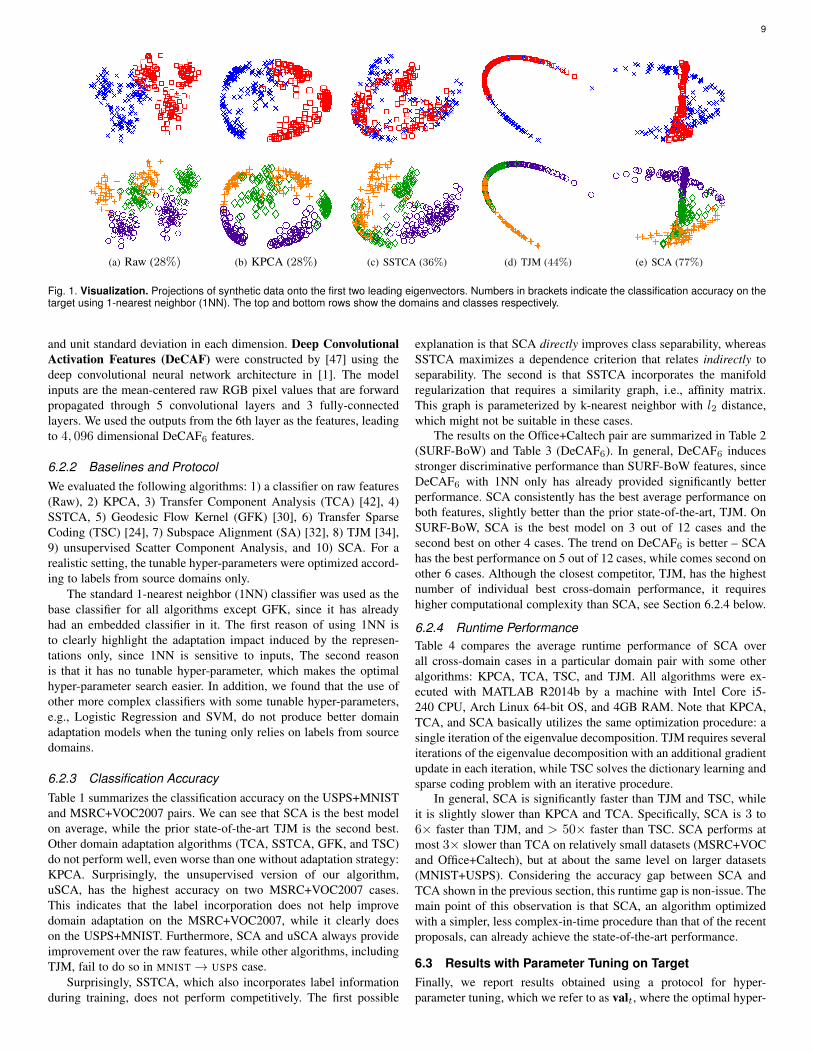
6.1 Synthetic dataFigure 1 depicts synthetic data that consists of two dimensional datapoints under three classes with six clusters. The data points in eachcluster were generated from a Gaussian distribution xci ∼ N (µc, σc),where µc and σc is the mean and standard deviation of the c-th cluster. The RBF kernel k(a,b) = exp(−‖a−b‖

22

σ2 ) was usedfor all algorithms. All tunable hyper-parameters were selected ac-cording to 1-nearest neighbor’s test accuracy. We compare featuresextracted from Kernel Principal Component Analysis (KPCA), Semi-Supervised Transfer Component Analysis (SSTCA) [42], TransferJoint Matching (TJM) [34], and SCA.

The top row of Figure 1 illustrates how the features extracted fromthe MMD-based algorithms (SSTCA, TJM, and SCA) reduce the

domain mismatch. Red and blue colors indicate the source and targetdomains, respectively. Good features for domain adaptation shouldhave a configuration of which the red and blue colors are mixed. Thiseffect can be seen in features extracted from SSTCA, TJM, and SCA,which indicates that the domain mismatch is successfully reduced inthe feature space. In classification, domain adaptive features shouldalso have a certain level of class separability. The bottom rowhighlights a major difference between SCA and the other algorithmsin terms of the class separability: the SCA features are more clusteredwith respect to the classes, with more prominent gaps among clusters.This suggests that it would be easier for a simple function to correctlyclassify SCA features.

6.2 Real world object recognition

We summarize the complete domain adaptation results over a rangeof cross-domain object recognition tasks. Several real-world imagedatasets were utilized such as handwritten digits (MNIST [67] andUSPS [68]) and general objects (MSRC [69], VOC2007 [6], Caltech-256 [70], Office [17]). Three cross-domain pairs were constructedfrom these datasets: USPS+MNIST, MSRC+VOC2007, and Of-fice+Caltech.

6.2.1 Data SetupThe USPS+MNIST pair consists of raw images subsampled fromdatasets of handwritten digits. MNIST contains 60,000 trainingimages and 10,000 test images of size 28 × 28. USPS has 7,291training images and 2,007 test images of size 16× 16 [67] . The pairwas constructed by randomly sampling 1,800 images from USPSand 2,000 images from MNIST. Images were uniformly rescaled tosize 16× 16 and encoded into feature vectors representing the gray-scale pixel values. Two SOURCE→ TARGET classification tasks wereconstructed: USPS→ MNIST and MNIST→ USPS.

The MSRC+VOC2007 pair consist of 240-dimensional imagesthat share 6 object categories: “aeroplane”, “bicycle”,“bird”, “car”,“cow”, and “sheep” taken from the MSRC and VOC2007 [6] datasets.The pair was constructed by selecting all 1,269 images in MSRCand 1,530 images in VOC2007. Feature were extracted from theraw pixels as follows. First, images were rescaled to be 16 × 16pixels. Second, 128-dimensional dense SIFT (DSIFT) features wereextracted using the VLFeat open source package [71]. Finally, a240-dimensional codebook was created using K-means clustering toobtain the codewords.

The Office+Caltech consists of 2,533 images of ten categories(8 to 151 images per category per domain), that forms four do-mains: (A) AMAZON, (D) DSLR, (W ) WEBCAM, and (C) CALTECH.AMAZON images were acquired in a controlled environment withstudio lighting. DSLR consists of high resolution images capturedby a digital SLR camera in a home environment under naturallighting. WEBCAM images were acquired in a similar environmentto DSLR, but with a low-resolution webcam. Finally, CALTECH

images were collected from Google Images [70]. Taking all possiblesource-target combinations yields 12 cross-domain datasets denotedby A → W,A → D,A → C, . . . , C → D. We used two typesof extracted features from these datasets that are publicly available:SURF-BoW2 [17] and DeCAF6

3 [47]. SURF-BoW features wereextracted using SURF [72] and quantized into 800-bin histogramswith codebooks computed by K-means on a subset of AMAZON

images. The final histograms were standardized to have zero mean

2. http://www-scf.usc.edu/∼boqinggo/da.html3. http://vc.sce.ntu.edu.sg/transfer learning domain adaptation/domain

adaptation home.html

9

(a) Raw (28%) (b) KPCA (28%) (c) SSTCA (36%) (d) TJM (44%) (e) SCA (77%)

Fig. 1. Visualization. Projections of synthetic data onto the first two leading eigenvectors. Numbers in brackets indicate the classification accuracy on thetarget using 1-nearest neighbor (1NN). The top and bottom rows show the domains and classes respectively.

and unit standard deviation in each dimension. Deep ConvolutionalActivation Features (DeCAF) were constructed by [47] using thedeep convolutional neural network architecture in [1]. The modelinputs are the mean-centered raw RGB pixel values that are forwardpropagated through 5 convolutional layers and 3 fully-connectedlayers. We used the outputs from the 6th layer as the features, leadingto 4, 096 dimensional DeCAF6 features.

6.2.2 Baselines and ProtocolWe evaluated the following algorithms: 1) a classifier on raw features(Raw), 2) KPCA, 3) Transfer Component Analysis (TCA) [42], 4)SSTCA, 5) Geodesic Flow Kernel (GFK) [30], 6) Transfer SparseCoding (TSC) [24], 7) Subspace Alignment (SA) [32], 8) TJM [34],9) unsupervised Scatter Component Analysis, and 10) SCA. For arealistic setting, the tunable hyper-parameters were optimized accord-ing to labels from source domains only.

The standard 1-nearest neighbor (1NN) classifier was used as thebase classifier for all algorithms except GFK, since it has alreadyhad an embedded classifier in it. The first reason of using 1NN isto clearly highlight the adaptation impact induced by the represen-tations only, since 1NN is sensitive to inputs, The second reasonis that it has no tunable hyper-parameter, which makes the optimalhyper-parameter search easier. In addition, we found that the use ofother more complex classifiers with some tunable hyper-parameters,e.g., Logistic Regression and SVM, do not produce better domainadaptation models when the tuning only relies on labels from sourcedomains.

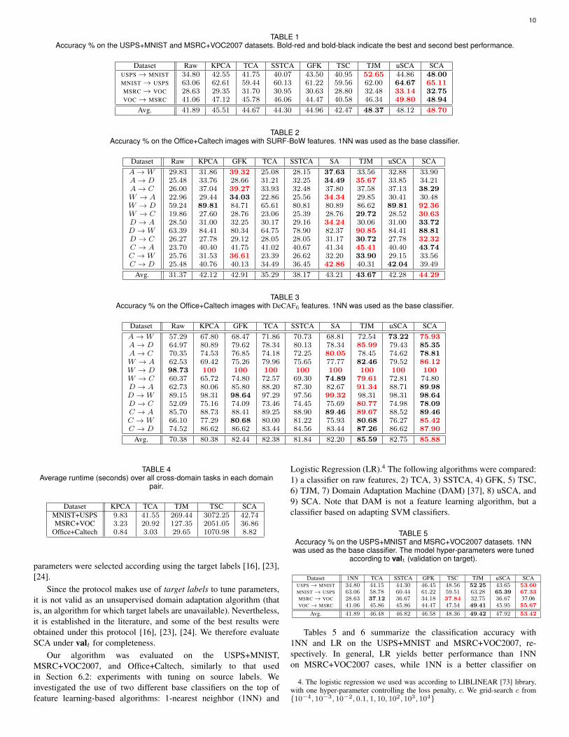
6.2.3 Classification AccuracyTable 1 summarizes the classification accuracy on the USPS+MNISTand MSRC+VOC2007 pairs. We can see that SCA is the best modelon average, while the prior state-of-the-art TJM is the second best.Other domain adaptation algorithms (TCA, SSTCA, GFK, and TSC)do not perform well, even worse than one without adaptation strategy:KPCA. Surprisingly, the unsupervised version of our algorithm,uSCA, has the highest accuracy on two MSRC+VOC2007 cases.This indicates that the label incorporation does not help improvedomain adaptation on the MSRC+VOC2007, while it clearly doeson the USPS+MNIST. Furthermore, SCA and uSCA always provideimprovement over the raw features, while other algorithms, includingTJM, fail to do so in MNIST → USPS case.

Surprisingly, SSTCA, which also incorporates label informationduring training, does not perform competitively. The first possible

explanation is that SCA directly improves class separability, whereasSSTCA maximizes a dependence criterion that relates indirectly toseparability. The second is that SSTCA incorporates the manifoldregularization that requires a similarity graph, i.e., affinity matrix.This graph is parameterized by k-nearest neighbor with l2 distance,which might not be suitable in these cases.

The results on the Office+Caltech pair are summarized in Table 2(SURF-BoW) and Table 3 (DeCAF6). In general, DeCAF6 inducesstronger discriminative performance than SURF-BoW features, sinceDeCAF6 with 1NN only has already provided significantly betterperformance. SCA consistently has the best average performance onboth features, slightly better than the prior state-of-the-art, TJM. OnSURF-BoW, SCA is the best model on 3 out of 12 cases and thesecond best on other 4 cases. The trend on DeCAF6 is better – SCAhas the best performance on 5 out of 12 cases, while comes second onother 6 cases. Although the closest competitor, TJM, has the highestnumber of individual best cross-domain performance, it requireshigher computational complexity than SCA, see Section 6.2.4 below.

6.2.4 Runtime PerformanceTable 4 compares the average runtime performance of SCA overall cross-domain cases in a particular domain pair with some otheralgorithms: KPCA, TCA, TSC, and TJM. All algorithms were ex-ecuted with MATLAB R2014b by a machine with Intel Core i5-240 CPU, Arch Linux 64-bit OS, and 4GB RAM. Note that KPCA,TCA, and SCA basically utilizes the same optimization procedure: asingle iteration of the eigenvalue decomposition. TJM requires severaliterations of the eigenvalue decomposition with an additional gradientupdate in each iteration, while TSC solves the dictionary learning andsparse coding problem with an iterative procedure.

In general, SCA is significantly faster than TJM and TSC, whileit is slightly slower than KPCA and TCA. Specifically, SCA is 3 to6× faster than TJM, and > 50× faster than TSC. SCA performs atmost 3× slower than TCA on relatively small datasets (MSRC+VOCand Office+Caltech), but at about the same level on larger datasets(MNIST+USPS). Considering the accuracy gap between SCA andTCA shown in the previous section, this runtime gap is non-issue. Themain point of this observation is that SCA, an algorithm optimizedwith a simpler, less complex-in-time procedure than that of the recentproposals, can already achieve the state-of-the-art performance.

6.3 Results with Parameter Tuning on TargetFinally, we report results obtained using a protocol for hyper-parameter tuning, which we refer to as valt, where the optimal hyper-

10

TABLE 1Accuracy % on the USPS+MNIST and MSRC+VOC2007 datasets. Bold-red and bold-black indicate the best and second best performance.

Dataset Raw KPCA TCA SSTCA GFK TSC TJM uSCA SCAUSPS→ MNIST 34.80 42.55 41.75 40.07 43.50 40.95 52.65 44.86 48.00MNIST→ USPS 63.06 62.61 59.44 60.13 61.22 59.56 62.00 64.67 65.11MSRC→ VOC 28.63 29.35 31.70 30.95 30.63 28.80 32.48 33.14 32.75VOC→ MSRC 41.06 47.12 45.78 46.06 44.47 40.58 46.34 49.80 48.94

Avg. 41.89 45.51 44.67 44.30 44.96 42.47 48.37 48.12 48.70

TABLE 2Accuracy % on the Office+Caltech images with SURF-BoW features. 1NN was used as the base classifier.

Dataset Raw KPCA GFK TCA SSTCA SA TJM uSCA SCAA→W 29.83 31.86 39.32 25.08 28.15 37.63 33.56 32.88 33.90A→ D 25.48 33.76 28.66 31.21 32.25 34.49 35.67 33.85 34.21A→ C 26.00 37.04 39.27 33.93 32.48 37.80 37.58 37.13 38.29W → A 22.96 29.44 34.03 22.86 25.56 34.34 29.85 30.41 30.48W → D 59.24 89.81 84.71 65.61 80.81 80.89 86.62 89.81 92.36W → C 19.86 27.60 28.76 23.06 25.39 28.76 29.72 28.52 30.63D → A 28.50 31.00 32.25 30.17 29.16 34.24 30.06 31.00 33.72D →W 63.39 84.41 80.34 64.75 78.90 82.37 90.85 84.41 88.81D → C 26.27 27.78 29.12 28.05 28.05 31.17 30.72 27.78 32.32C → A 23.70 40.40 41.75 41.02 40.67 41.34 45.41 40.40 43.74C →W 25.76 31.53 36.61 23.39 26.62 32.20 33.90 29.15 33.56C → D 25.48 40.76 40.13 34.49 36.45 42.86 40.31 42.04 39.49

Avg. 31.37 42.12 42.91 35.29 38.17 43.21 43.67 42.28 44.29

TABLE 3Accuracy % on the Office+Caltech images with DeCAF6 features. 1NN was used as the base classifier.

Dataset Raw KPCA GFK TCA SSTCA SA TJM uSCA SCAA→W 57.29 67.80 68.47 71.86 70.73 68.81 72.54 73.22 75.93A→ D 64.97 80.89 79.62 78.34 80.13 78.34 85.99 79.43 85.35A→ C 70.35 74.53 76.85 74.18 72.25 80.05 78.45 74.62 78.81W → A 62.53 69.42 75.26 79.96 75.65 77.77 82.46 79.52 86.12W → D 98.73 100 100 100 100 100 100 100 100W → C 60.37 65.72 74.80 72.57 69.30 74.89 79.61 72.81 74.80D → A 62.73 80.06 85.80 88.20 87.30 82.67 91.34 88.71 89.98D →W 89.15 98.31 98.64 97.29 97.56 99.32 98.31 98.31 98.64D → C 52.09 75.16 74.09 73.46 74.45 75.69 80.77 74.98 78.09C → A 85.70 88.73 88.41 89.25 88.90 89.46 89.67 88.52 89.46C →W 66.10 77.29 80.68 80.00 81.22 75.93 80.68 76.27 85.42C → D 74.52 86.62 86.62 83.44 84.56 83.44 87.26 86.62 87.90

Avg. 70.38 80.38 82.44 82.38 81.84 82.20 85.59 82.75 85.88

TABLE 4Average runtime (seconds) over all cross-domain tasks in each domain

pair.

Dataset KPCA TCA TJM TSC SCAMNIST+USPS 9.83 41.55 269.44 3072.25 42.74MSRC+VOC 3.23 20.92 127.35 2051.05 36.86

Office+Caltech 0.84 3.03 29.65 1070.98 8.82

parameters were selected according using the target labels [16], [23],[24].

Since the protocol makes use of target labels to tune parameters,it is not valid as an unsupervised domain adaptation algorithm (thatis, an algorithm for which target labels are unavailable). Nevertheless,it is established in the literature, and some of the best results wereobtained under this protocol [16], [23], [24]. We therefore evaluateSCA under valt for completeness.

Our algorithm was evaluated on the USPS+MNIST,MSRC+VOC2007, and Office+Caltech, similarly to that usedin Section 6.2: experiments with tuning on source labels. Weinvestigated the use of two different base classifiers on the top offeature learning-based algorithms: 1-nearest neighbor (1NN) and

Logistic Regression (LR).4 The following algorithms were compared:1) a classifier on raw features, 2) TCA, 3) SSTCA, 4) GFK, 5) TSC,6) TJM, 7) Domain Adaptation Machine (DAM) [37], 8) uSCA, and9) SCA. Note that DAM is not a feature learning algorithm, but aclassifier based on adapting SVM classifiers.

TABLE 5Accuracy % on the USPS+MNIST and MSRC+VOC2007 datasets. 1NN

was used as the base classifier. The model hyper-parameters were tunedaccording to valt (validation on target).

Dataset 1NN TCA SSTCA GFK TSC TJM uSCA SCAUSPS→ MNIST 34.80 44.15 44.30 46.45 48.56 52.25 43.65 53.60MNIST→ USPS 63.06 58.78 60.44 61.22 59.51 63.28 65.39 67.33MSRC→ VOC 28.63 37.12 36.67 34.18 37.84 32.75 36.67 37.06VOC→ MSRC 41.06 45.86 45.86 44.47 47.54 49.41 45.95 55.67

Avg. 41.89 46.48 46.82 46.58 48.36 49.42 47.92 53.42

Tables 5 and 6 summarize the classification accuracy with1NN and LR on the USPS+MNIST and MSRC+VOC2007, re-spectively. In general, LR yields better performance than 1NNon MSRC+VOC2007 cases, while 1NN is a better classifier on

4. The logistic regression we used was according to LIBLINEAR [73] library,with one hyper-parameter controlling the loss penalty, c. We grid-search c from{10−4, 10−3, 10−2, 0.1, 1, 10, 102, 103, 104}

11

TABLE 6Accuracy % on the USPS+MNIST and MSRC+VOC2007 datasets.

Logistic Regression (LR) was used as the base classifier for TCA, TSC,TJM, and SCA. The model hyper-parameters were tuned according to valt

(validation on target).

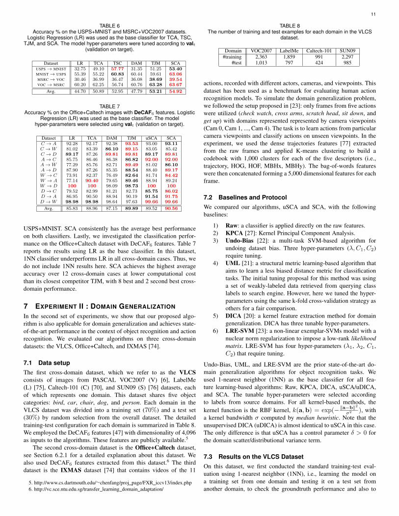
Dataset LR TCA TSC DAM TJM SCAUSPS→ MNIST 32.75 49.10 57.77 31.35 51.25 53.40MNIST→ USPS 55.39 55.22 60.83 60.44 59.61 63.06MSRC→ VOC 30.46 36.99 36.47 36.08 38.69 39.54VOC→ MSRC 60.20 62.25 56.74 60.76 63.28 63.67

Avg. 44.70 50.89 52.95 47.79 53.21 54.92

TABLE 7Accuracy % on the Office+Caltech images with DeCAF6 features. Logistic

Regression (LR) was used as the base classifier. The modelhyper-parameters were selected using valt (validation on target).

Dataset LR TCA DAM TJM uSCA SCAC → A 92.28 92.17 92.38 93.53 93.00 93.11C →W 81.02 83.39 86.10 89.15 83.05 85.42C → D 89.17 87.26 89.81 89.81 89.17 89.81A→ C 85.75 86.46 86.38 86.82 92.00 92.00A→W 77.29 85.76 82.71 89.49 81.02 86.10A→ D 87.90 87.26 85.35 88.54 88.40 89.17W → C 73.91 82.37 76.49 82.64 81.74 84.42W → A 77.14 90.40 79.65 89.46 88.94 89.24W → D 100 100 98.09 98.73 100 100D → C 79.52 82.99 81.21 82.73 85.75 86.02D → A 86.95 90.50 88.94 90.19 91.54 91.75D →W 98.98 98.98 98.64 97.63 99.66 99.66

Avg. 85.83 88.96 87.15 89.89 89.52 90.56

USPS+MNIST. SCA consistently has the average best performanceon both classifiers. Lastly, we investigated the classification perfor-mance on the Office+Caltech dataset with DeCAF6 features. Table 7reports the results using LR as the base classifier. In this dataset,1NN classifier underperforms LR in all cross-domain cases. Thus, wedo not include 1NN results here. SCA achieves the highest averageaccuracy over 12 cross-domain cases at lower computational costthan its closest competitor TJM, with 8 best and 2 second best cross-domain performance.

7 EXPERIMENT II : DOMAIN GENERALIZATION

In the second set of experiments, we show that our proposed algo-rithm is also applicable for domain generalization and achieves state-of-the-art performance in the context of object recognition and actionrecognition. We evaluated our algorithms on three cross-domaindatasets: the VLCS, Office+Caltech, and IXMAS [74].

7.1 Data setupThe first cross-domain dataset, which we refer to as the VLCSconsists of images from PASCAL VOC2007 (V) [6], LabelMe(L) [75], Caltech-101 (C) [70], and SUN09 (S) [76] datasets, eachof which represents one domain. This dataset shares five objectcategories: bird, car, chair, dog, and person. Each domain in theVLCS dataset was divided into a training set (70%) and a test set(30%) by random selection from the overall dataset. The detailedtraining-test configuration for each domain is summarized in Table 8.We employed the DeCAF6 features [47] with dimensionality of 4,096as inputs to the algorithms. These features are publicly available.5

The second cross-domain dataset is the Office+Caltech dataset,see Section 6.2.1 for a detailed explanation about this dataset. Wealso used DeCAF6 features extracted from this dataset.6 The thirddataset is the IXMAS dataset [74] that contains videos of the 11

5. http://www.cs.dartmouth.edu/∼chenfang/proj page/FXR iccv13/index.php6. http://vc.sce.ntu.edu.sg/transfer learning domain adaptation/

TABLE 8The number of training and test examples for each domain in the VLCS

dataset.

Domain VOC2007 LabelMe Caltech-101 SUN09#training 2,363 1,859 991 2,297

#test 1,013 797 424 985

actions, recorded with different actors, cameras, and viewpoints. Thisdataset has been used as a benchmark for evaluating human actionrecognition models. To simulate the domain generalization problem,we followed the setup proposed in [23]: only frames from five actionswere utilized (check watch, cross arms, scratch head, sit down, andget up) with domains represented represented by camera viewpoints(Cam 0, Cam 1, ..., Cam 4). The task is to learn actions from particularcamera viewpoints and classify actions on unseen viewpoints. In theexperiment, we used the dense trajectories features [77] extractedfrom the raw frames and applied K-means clustering to build acodebook with 1,000 clusters for each of the five descriptors (i.e.,trajectory, HOG, HOF, MBHx, MBHy). The bag-of-words featureswere then concatenated forming a 5,000 dimensional features for eachframe.

7.2 Baselines and ProtocolWe compared our algorithms, uSCA and SCA, with the followingbaselines:

1) Raw: a classifier is applied directly on the raw features.2) KPCA [27]: Kernel Principal Component Analysis.3) Undo-Bias [22]: a multi-task SVM-based algorithm for

undoing dataset bias. Three hyper-parameters (λ,C1, C2)require tuning.

4) UML [21]: a structural metric learning-based algorithm thataims to learn a less biased distance metric for classificationtasks. The initial tuning proposal for this method was usinga set of weakly-labeled data retrieved from querying classlabels to search engine. However, here we tuned the hyper-parameters using the same k-fold cross-validation strategy asothers for a fair comparison.

5) DICA [20]: a kernel feature extraction method for domaingeneralization. DICA has three tunable hyper-parameters.

6) LRE-SVM [23]: a non-linear exemplar-SVMs model with anuclear norm regularization to impose a low-rank likelihoodmatrix. LRE-SVM has four hyper-parameters (λ1, λ2, C1,C2) that require tuning.

Undo-Bias, UML, and LRE-SVM are the prior state-of-the-art do-main generalization algorithms for object recognition tasks. Weused 1-nearest neighbor (1NN) as the base classifier for all fea-ture learning-based algorithms: Raw, KPCA, DICA, uSCA/uDICA,and SCA. The tunable hyper-parameters were selected accordingto labels from source domains. For all kernel-based methods, thekernel function is the RBF kernel, k(a,b) = exp(−‖a−b‖

2

σ2 ), witha kernel bandwidth σ computed by median heuristic. Note that theunsupervised DICA (uDICA) is almost identical to uSCA in this case.The only difference is that uSCA has a control parameter δ > 0 forthe domain scatter/distributional variance term.

7.3 Results on the VLCS DatasetOn this dataset, we first conducted the standard training-test eval-uation using 1-nearest neighbor (1NN), i.e., learning the model ona training set from one domain and testing it on a test set fromanother domain, to check the groundtruth performance and also to

12

TABLE 9The groundtruth 1NN accuracy % of five-class classification when training on one dataset (the left-most column) and testing on another (the upper-most

row). The bold black numbers indicate in-domain performance, while the plain black indicate cross-domain performance. “Self” refers to training andtesting on the same dataset, same as the bold black numbers and “mean others” refers to the average performance over all cross-domain cases. Dividing

“self” and “mean others” results in the (percent) performance drop indicated by the red color.

Training/Test VOC2007 LabelMe Caltech-101 SUN09 Self Mean others Percent dropVOC2007 72.46 52.45 89.17 60.00 72.46 67.20 ∼ 7%LabelMe 54.99 63.74 79.72 46.90 63.74 60.54 ∼ 5%

Caltech-101 53.70 44.79 99.53 44.87 99.53 47.49 ∼ 52%SUN09 51.63 50.69 50.71 68.12 68.12 51.01 ∼ 25%

Mean others 53.44 49.31 73.19 50.59 75.96 56.63 ∼ 25%

TABLE 10The domain generalization performance accuracy (%) on the VLCS dataset with DeCAF6 features as inputs. The accuracy of all feature learning-based

algorithms: Raw, KPCA, uSCA, DICA, SCA is according to 1-nearest neighbor (1NN) classifier. Bold red and bold black indicate the best and the secondbest performance, respectively.

Source Target Raw KPCA Undo-Bias UML LRE-SVM uSCA DICA SCAL,C,S V 57.26 60.22 54.29 56.26 60.58 58.54 59.62 64.36V,C,S L 52.45 51.94 58.09 58.50 59.74 54.08 51.82 59.60V,L,S C 90.57 90.09 87.50 91.13 88.11 85.14 78.30 88.92V,L,C S 56.95 55.03 54.21 58.49 54.88 55.63 55.33 59.29C,S V,L 55.08 55.64 59.28 56.47 55.04 53.98 50.90 59.50C,L V,S 52.60 50.70 55.80 54.72 52.87 49.05 55.47 55.96V,C L,S 56.62 54.66 62.35 55.49 58.84 55.89 58.08 60.77

Avg. 60.22 59.47 61.65 61.58 61.44 58.90 58.50 64.06

TABLE 11The domain generalization performance accuracy (%) on the Office+Caltech dataset with DeCAF6 features as inputs.

Source Target Raw KPCA Undo-Bias UML LRE-SVM uSCA DICA SCAW, D, C A 85.39 89.14 90.98 91.02 91.87 89.46 90.40 92.38A,W,D C 73.73 75.87 85.95 84.59 86.38 77.15 84.33 86.73

A,C D,W 67.92 78.99 80.49 82.29 84.59 78.10 79.65 85.84D,W A,C 67.09 68.84 69.98 79.54 81.17 71.74 69.73 75.54

Avg. 72.28 77.71 81.85 84.36 86.00 79.11 81.02 85.12

TABLE 12The domain generalization performance accuracy (%) on the IXMAS dataset with dense trajectory-based features.

Source Target Raw KPCA Undo-Bias UML LRE-SVM uSCA DICA SCACam 0,1 Cam 2,3,4 58.24 67.77 69.03 74.14 79.96 66.67 65.93 80.59

Cam 2,3,4 Cam 0,1 20.33 41.21 60.56 63.79 80.15 51.09 78.02 85.16Cam 0,1,2,3 Cam 4 58.24 59.34 56.84 60.37 74.97 61.54 62.64 70.33

Avg. 45.60 56.10 62.14 66.10 78.36 59.77 68.86 78.69

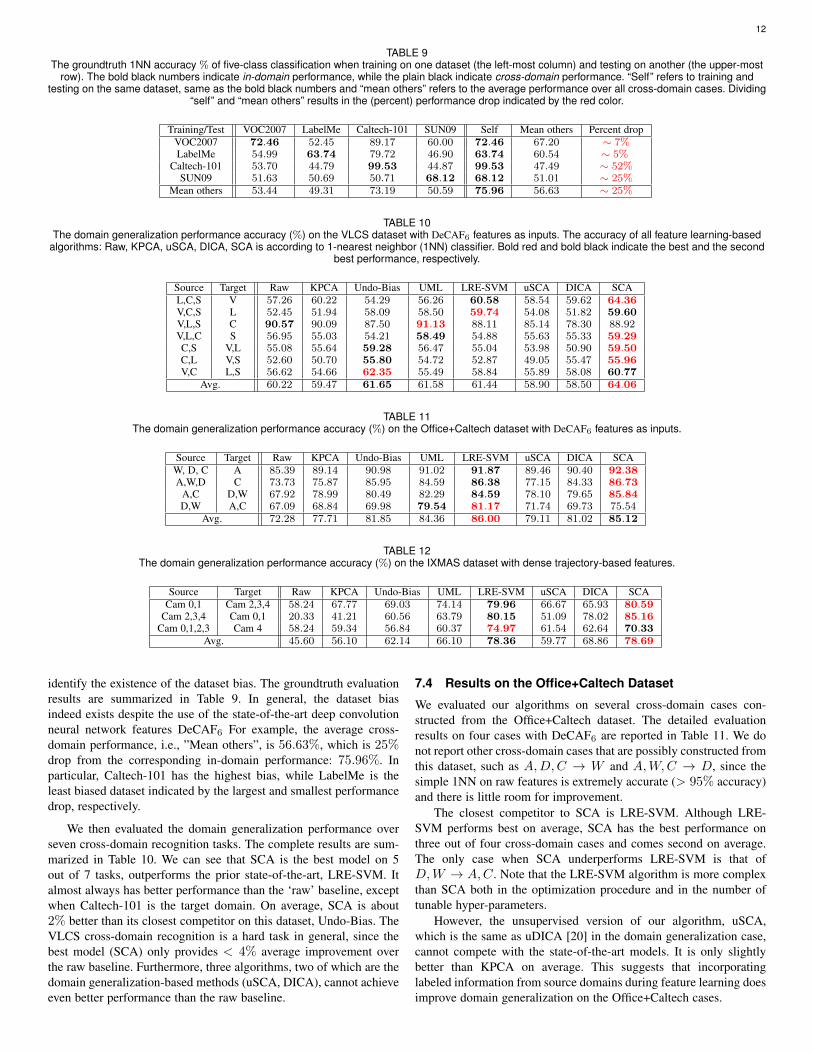
identify the existence of the dataset bias. The groundtruth evaluationresults are summarized in Table 9. In general, the dataset biasindeed exists despite the use of the state-of-the-art deep convolutionneural network features DeCAF6 For example, the average cross-domain performance, i.e., ”Mean others”, is 56.63%, which is 25%drop from the corresponding in-domain performance: 75.96%. Inparticular, Caltech-101 has the highest bias, while LabelMe is theleast biased dataset indicated by the largest and smallest performancedrop, respectively.

We then evaluated the domain generalization performance overseven cross-domain recognition tasks. The complete results are sum-marized in Table 10. We can see that SCA is the best model on 5out of 7 tasks, outperforms the prior state-of-the-art, LRE-SVM. Italmost always has better performance than the ‘raw’ baseline, exceptwhen Caltech-101 is the target domain. On average, SCA is about2% better than its closest competitor on this dataset, Undo-Bias. TheVLCS cross-domain recognition is a hard task in general, since thebest model (SCA) only provides < 4% average improvement overthe raw baseline. Furthermore, three algorithms, two of which are thedomain generalization-based methods (uSCA, DICA), cannot achieveeven better performance than the raw baseline.

7.4 Results on the Office+Caltech Dataset

We evaluated our algorithms on several cross-domain cases con-structed from the Office+Caltech dataset. The detailed evaluationresults on four cases with DeCAF6 are reported in Table 11. We donot report other cross-domain cases that are possibly constructed fromthis dataset, such as A,D,C → W and A,W,C → D, since thesimple 1NN on raw features is extremely accurate (> 95% accuracy)and there is little room for improvement.

The closest competitor to SCA is LRE-SVM. Although LRE-SVM performs best on average, SCA has the best performance onthree out of four cross-domain cases and comes second on average.The only case when SCA underperforms LRE-SVM is that ofD,W → A,C. Note that the LRE-SVM algorithm is more complexthan SCA both in the optimization procedure and in the number oftunable hyper-parameters.

However, the unsupervised version of our algorithm, uSCA,which is the same as uDICA [20] in the domain generalization case,cannot compete with the state-of-the-art models. It is only slightlybetter than KPCA on average. This suggests that incorporatinglabeled information from source domains during feature learning doesimprove domain generalization on the Office+Caltech cases.

13

7.5 Results on the IXMAS datasetTable 12 summarizes the classification accuracies on the IXMASdataset over three cross-domain cases. We can see that the standardbaselines (Raw, KPCA) cannot match other algorithms with domaingeneralization strategies. In this dataset, SCA has the best perfor-mance on two out of three cases and on average. In particular, SCA issignificantly better than others on Cam 2,3,4→ Cam 0,1 case. LRE-SVM remains the closest competitor of SCA – it has the second bestaverage performance with one best cross-domain case.

7.6 Runtime PerformanceNext we report the average (training) runtime performance overall cross-domain recognition tasks in each dataset. All algorithmswere executed using the same software and machine as describedin Section 6.2.4. From Table 13, we can see that the runtime ofSCA is on par with KPCA and DICA, which is expected sincethey utilize the same optimization procedure: a single run with ageneralized eigenvalue decomposition. In the previous subsections,we have shown that SCA provides better performance accuracy thanKPCA and DICA.

SCA is significantly faster than some prior state-of-the-art do-main generalization methods (Undo-Bias, UML, and LRE-SVM).For example, on the VLCS dataset, Undo-Bias, UML, and LRE-SVM require ∼ 30 minutes, while SCA only needs ∼ 5 minutesaverage training time. An analogous trend can also be seen in thecase of Office+Caltech and IXMAS datasets. This outcome indicatesthat SCA is better suited for domain generalization tasks than thecompeting algorithms if a training stage in real time is required.

TABLE 13Average domain generalization runtime (seconds) over all cross-domain

recognition tasks in each dataset.

Dataset KPCA Undo-Bias DICA UML LRE-SVM SCAVLCS 201.99 1, 925.54 336.92 1, 652.67 2, 161.60 300.94

Office+Caltech 6.53 589.50 17.90 413.25 695.31 18.49IXMAS 0.50 49.14 0.79 57.67 65.47 0.96

8 CONCLUSIONS

The scatter-based objective function is a straightforward way toencode the relevant structure of the domain adaptation and domaingeneralization problems. SCA uses variances between subsets of thedata to construct a linear transformation that dampens unimportantdistinctions (within labels and between domains) and amplifies usefuldistinctions (between labels and overall variability). Extensive experi-ments on several cross-domain image datasets show that SCA is muchfaster than competing algorithms and provides the state-of-the-artperformance on both domain adaptation and domain generalization.

Our theoretical analysis shows that scatter with two input do-mains, i.e., domain scatter, relates to generalization bounds fordomain adaptation [28]. In the setting of domain adaptation, recallremark 1, prior work has shown that the distributional variance (whichis a special case of scatter) arises as one of the terms controllinggeneralization performance [20]. Scatter thus unifying quantity thatcontrols generalization performance in for domain adaptation andgeneralization.

SCA is a natural extension of Kernel PCA, Kernel Fisher Dis-criminant and TCA. In contrast, many domain adaptation methodsuse objective functions that combine the total variance and MMDwith quantities that are fundamentally different in kind such as thegraph Laplacian [24], sparsity constraints [24], [34], the Hilbert-Schmidt independence criterion [42] or the central subspace [20].SCA can easily be extended to semi-supervised domain adaptation, by

incorporating target labels into the class scatters. Finally, we remarkthat it should be possible to speed up SCA for large-scale problemsusing random features [78], [79].

In general, the domain adaptation and domain generalizationproblem, that is, dataset bias, remains far from solved. The actualsatisfactory performance of existing algorithms (≥ 80% accuracy)is achieved only in several cross-domain tasks, even using powerfulfeature extraction methods such as DeCAF6 (for images) and densetrajectory-based features (for videos). The use of less powerfulfeatures (raw pixels or SURF-BoW) is clearly unsatisfactory. Thus,it is crucial to develop more fundamental feature learning algorithmsthat can significantly reduce dataset bias in all situations.

9 ACKNOWLEDGMENTS

The authors would like to thank Zheng Xu for sharing the extracteddense trajectories features from the IXMAS dataset, and also ChenFang for sharing the Unbiased Metric Learning code and usefuldiscussions.

REFERENCES

[1] A. Krizhevsky, I. Sutskever, and G. E. Hinton, “Classification with DeepConvolutional Neural Networks,” in NIPS, vol. 25, 2012, pp. 1106–1114.

[2] K. Simonyan and A. Zisserman, “Very deep convolutional networks forlarge-scale image recognition,” in Proceedings of International Conferenceon Learning Representations, 2015.

[3] R. Girshick, J. Donahue, T. Darrell, and J. Malik, “Rich feature hierarchiesfor accurate object detection and semantic segmentation,” in Computer Visionand Pattern Recognition (CVPR), 2014.

[4] G. E. Dahl, T. N. Sainath, and G. Hinton, “Improving deep neural networksfor LVCSR using rectified linear units and dropout,” in ICASSP, 2013.

[5] I. Sutskever, O. Vinyals, and Q. Le, “Sequence to Sequence Learning withNeural Networks,” in NIPS, 2014.

[6] M. Everingham, L. Van-Gool, C. K. I. Williams, J. Winn, and A. Zisserman,“The PASCAL Visual Object Classes Challenge 2007 Results,” 2007.

[7] A. Krizhevsky, “Learning Multiple Layers of Features from Tiny Images,”Master’s thesis, Department of Computer Science, University of Toronto,Apr. 2009.

[8] J. Ponce, T. L. Berg, M. Everingham, D. A. Forsyth, M. Hebert, S. Lazebnik,M. Marsza?ek, C. Schmid, B. C. Russell, A. Torralba, C. K. I. Williams,J. Zhang, and A. Zisserman, “Dataset issues in object recognition,” in TowardCategory-Level Object Recognition, 2006, vol. 4170, pp. 29–48.

[9] A. Torralba and A. A. Efros, “Unbiased Look at Dataset Bias,” in CVPR,2011, pp. 1521–1528.

[10] J. Blitzer, R. McDonald, and F. Pereira, “Domain Adaptation with StructuralCorrespondence Learning,” in Proceedings of the 2006 Conference onEmpirical Methods in Natural Language Processing, 2006, pp. 120–128.

[11] G. Blanchard, G. Lee, and C. Scott, “Generalizing from Several RelatedClassification Tasks to a New Unlabeled Sample,” in NIPS, 2011, pp. 2178–2186.

[12] J. Blitzer, M. Dredze, and F. Pereira, “Biographies, bollywood, boom-boxesand blenders: Domain adaptation for sentiment classification,” in Associationfor Computational Linguistics (ACL), 2007.

[13] M. Chen, Z. Xu, K. Weinberger, and F. Sha, “Marginalized DenoisingAutoencoders for Domain Adaptation,” in ICML, 2012, pp. 767–774.

[14] X. Glorot, A. Bordes, and Y. Bengio, “Domain Adaptation for Large-ScaleSentiment Classification: A Deep Learning Approach,” in Proceedings ofthe 28th International Conference on Machine Learning (ICML), 2011, pp.513–520.

[15] J. Hoffman, E. Rodner, J. Donahue, T. Darrell, and K. Saenko, “EfficientLearning of Domain-invariant Image Representations,” in ICLR, 2013.

[16] M. Long, J. Wang, G. Ding, D. Shen, and Q. Yang, “Transfer Learningwith Graph Co-Regularization,” IEEE Transactions on Knowledge and DataEngineering, vol. 26, no. 7, pp. 1805–1818, 2014.

[17] K. Saenko, B. Kulis, M. Fritz, and T. Darrell, “Adapting Visual CategoryModels to New Domains,” in ECCV, 2010, pp. 213–226.

[18] S. Shekhar, V. M. Patel, H. V. Nguyen, and R. Chellapa, “Generalizeddomain-adaptive dictionaries,” in IEEE Conference on Computer Vision andPattern Recognition, 2013, pp. 361–368.

[19] S. J. Pan, I. W. Tsang, J. T. Kwok, and Q. Yang, “Domain adaptation viatransfer component analysis,” in IJCAI, 2009, pp. 1187–1192.

[20] K. Muandet, D. Balduzzi, and B. Scholkopf, “Domain Generalization viaInvariant Feature Representation,” in ICML, vol. 28, 2013, pp. 10–18.

14

[21] C. Fang, Y. Xu, and D. N. Rockmore, “Unbiased Metric Learning: On theUtilization of Multiple Datasets and Web Images for Softening Bias,” inICCV, 2013, pp. 1657–1664.

[22] A. Khosla, T. Zhou, T. Malisiewicz, A. Efros, and A. Torralba, “Undoing theDamage of Dataset Bias,” in ECCV, vol. I, 2012, pp. 158–171.

[23] Z. Xu, W. Li, L. Niu, and D. Xu, “Exploiting Low-Rank Structure fromLatent Domains for Domain Generalization,” in European Conference onComputer Vision (ECCV), 2014, pp. 628–643.

[24] M. Long, G. Ding, J. Wang, J. Sun, Y. Guo, and P. S. Yu, “Transfer SparseCoding for Robust Image Representation,” in CVPR, 2013, pp. 404–414.

[25] R. A. Fisher, “The Use of Multiple Measurements in Taxonomic Problems,”Annals of Eugenics, vol. 7, pp. 179–188, 1936.

[26] K. M. Borgwardt, A. Gretton, M. J. Rasch, H.-P. Kriegel, B. Scholkopf, andA. J. Smola, “Integrating structured biological data by Kernel MaximumMean Discrepancy,” Bioinformatics, vol. 22, no. 14, pp. e49–e57, 2006.

[27] B. Scholkopf, A. Smola, and K.-R. Muller, “Nonlinear Component Analysisas a Kernel Eigenvalue Problem,” Neural Computation, vol. 10, no. 5, pp.1299–1319, 1998.

[28] Y. Mansour, M. Mohri, and A. Rostamizadeh, “Domain adaptation: Learningbounds and algorithms,” in Conference on Learning Theory (COLT), 2009.

[29] J. Jiang, “A Literature Survey on Domain Adaptation of StatisticalClassifiers,” Available at http://sifaka.cs.uiuc.edu/jiang4/domain adaptation/survey, 2008.

[30] B. Gong, Y. Shi, F. Sha, and K. Grauman, “Geodesic Flow Kernel forUnsupervised Domain Adaptation,” in CVPR, 2012, pp. 2066–2073.

[31] T. Tommasi and B. Caputo, “Frustratingly Easy NBNN Domain Adaptation,”in ICCV, 2013, pp. 897–904.

[32] B. Fernando, A. Habrard, M. Sebban, and T. Tuytelaars, “UnsupervisedVisual Domain Adaptation Using Subspace Alignment,” in ICCV, 2013, pp.2960–2967.

[33] J. Hoffman, T. Darrell, and K. Saenko, “Continuous Manifold Based Adap-tation for Evolving Visual Domains,” in CVPR, 2014.

[34] M. Long, J. Wang, G. Ding, J. Sun, and P. S. Yu, “Transfer Joint Matchingfor Unsupervised Domain Adaptation,” in CVPR, 2014, pp. 1410–1417.

[35] V. M. Patel, R. Gopalan, R. Li, and R. Chellapa, “Visual domain adaptation:A survey of recent advances,” IEEE Signal Processing Magazine, vol. 32,no. 3, pp. 53–69, 2015.

[36] J. Yang, R. Yan, and A. G. Hauptmann, “Cross-domain video conceptdetection using adaptive SVMs,” in Proc of 15th Int Conf on Multimedia,2007, pp. 188–197.

[37] L. Duan, I. W. Tsang, and D. Xu, “Domain Adaptation from Multiple Sourcesvia Auxiliary Classifiers,” in ICML, 2009, pp. 289–296.

[38] T. van Gestel, B. B. Suykens, Johan A. K., S. Viaene, J. Vanthienen,G. Dedene, B. de Moor, and J. Vandewalle, “Benchmarking least squaressupport vector machine classifiers,” Machine Learning, vol. 54, no. 1, pp.5–32, 2004.

[39] H. Shimodaira, “Improving predictive inference under covariate shift byweighting the log-likelihood function,” Journal of Statistical Planning andInference, vol. 90, no. 2, pp. 227–244, 2000.

[40] B. Gong, K. Grauman, and F. Sha, “Connecting the Dots with Landmarks:Discriminatively Learning Domain-Invariant Features for Unsupervised Do-main Adaptation,” in Proceedings of the International Conference on Ma-chine Learning (ICML), 2013.

[41] A. Gretton, K. M. Borgwardt, M. Rasch, B. Scholkopf, and A. J. Smola,“A Kernel Method for the Two-Sample-Problem,” in Advances in NeuralInformation Processing System 19 (NIPS), 2007, pp. 513–520.

[42] S. J. Pan, I. W.-H. Tsang, J. T. Kwok, and Q. Yang, “Domain adaptation viatransfer component analysis,” IEEE Trans. Neural Networks, vol. 22, no. 2,pp. 199–210, 2011.

[43] B. Kulis, K. Saenko, and T. Darrell, “What You Saw is Not What You Get:Domain Adaptation Using Asymmetric Kernel Transforms,” in CVPR, 2011,pp. 1785–1792.

[44] R. Gopalan, R. Li, and R. Chellapa, “Domain Adaptation for Object Recog-nition: An Unsupervised Approach,” in ICCV, 2011, pp. 999–1006.

[45] S. Chopra, S. Balakrishnan, and R. Gopalan, “DLID: Deep Learning forDomain Adaptation by Interpolating between Domains,” in ICML Workshopon Challenges in Representation Learning, 2013.

[46] H. V. Nguyen, H. T. Ho, V. M. Patel, and R. Chellapa, “Joint HierarchicalDomain Adaptation and Feature Learning,” IEEE Transactions on ImageProcessing, 2015.

[47] J. Donahue, Y. Jia, O. Vinyals, J. Hoffman, N. Zhang, E. Tzeng, andT. Darrell, “DeCAF: A Deep Convolutional Activation Feature for GenericVisual Recognition,” in ICML, 2014.

[48] M. Ghifary, W. B. Kleijn, and M. Zhang, “Domain adaptive neural networksfor object recognition,” in PRICAI: Trends in AI, vol. 8862, 2014, pp. 898–904.

[49] M. Long, Y. Cao, J. Wang, and M. I. Jordan, “Learning transferable featureswith deep adaptation networks,” in Proceedings of the 32nd InternationalConference on Machine Learning, 2015.

[50] S. Ben-David, J. Blitzer, K. Crammer, and F. Pereira, “Analysis of Rep-resentations for Domain Adaptation,” in Advances in Neural InformationProcessing Systems (NIPS), 2007, pp. 137–144.

[51] P. L. Bartlett and S. Mendelson, “Rademacher and gaussian complexities:Risk bounds and structural results,” Journal of Machine Learning Research,2002.

[52] M. Kim and V. Pavlovic, “Central Subspace Dimensionality Reduction UsingCovariance Operators,” IEEE Transactions on Pattern Analysis and MachineIntelligence, vol. 33, no. 4, pp. 657–670, 2011.

[53] T. Malisiewicz, A. Gupta, and A. A. Efros, “Ensemble of Exemplar-SVMs for Object Detection and Beyond,” in Proceedings of InternationalConference on Computer Vision, 2011.

[54] A. Smola, A. Gretton, L. Song, and B. Scholkopf, “A Hilbert SpaceEmbedding for Distributions,” in ALT, 2007.

[55] C. McDiarmid, “On the Method of Bounded Differences,” Surveys inCombinatorics, vol. 141, no. 148-188, 1989.

[56] J. Huang, A. J. Smola, A. Gretton, and S. B. Borgwardt, Karsten M.,“Correcting sample selection bias by unlabeled data,” in Advances in NeuralInformation Processing Systems 19 (NIPS), 2007, pp. 601–608.

[57] B. K. Sriperumbudur, A. Gretton, K. Fukumizu, B. Scholkopf, and G. R. G.Lanckriet, “Hilbert space embeddings and metrics on probability measures,”Journal of Machine Learning Research, vol. 99, pp. 1517–1561, 2010.

[58] A. Gretton, K. M. Borgwardt, M. J. Rasch, B. Scholkopf, and A. Smola, “AKernel Two-Sample Test,” JMLR, pp. 723–773, 2012.

[59] S. Mika, G. Ratsch, J. Weston, B. Scholkopf, and K.-R. Muller, “Fisher dis-criminant analysis with kernels,” in Neural Networks for Signal ProcessingIX, 1999, pp. 41–48.

[60] B. Geng, D. Tao, and C. Xu, “DAML: Domain Adaptation Metric Learning,”IEEE Transactions on Image Processing, vol. 20, no. 10, pp. 2980–2989,2011.

[61] I. Steinwart, “On the influence of the kernel on the consistency of supportvector machines,” Journal of Machine Learning Research, vol. 2, pp. 67–93,2002.

[62] C. Cortes and M. Mohri, “Domain adaptation and sample bias correctiontheory and algorithm for regression,” Theoretical Computer Science, vol.519, pp. 103–126, 2014.

[63] Steffen Grunewalder and Arthur Gretton and John Shawe-Taylor, “SmoothOperators,” in ICML, 2013.

[64] C. A. Micchelli, Y. Xu, and H. Zhang, “Universal Kernels,” JMLR, vol. 7,pp. 2651–2667, 2006.

[65] M. Mohri, A. Rostamizadeh, and A. Talwalkar, Foundations of MachineLearning. The MIT Press, 2012.

[66] M. Ledoux and M. Talagrand, Probability in Banach Space. Springer-Verlag, New York, 1991.

[67] Y. LeCun, L. Bottou, Y. Bengio, and P. Haffner, “Gradient-based learningapplied to document recognition,” in Proceedings of the IEEE, vol. 86,no. 11, 1998, pp. 2278–2324.

[68] J. J. Hull, “A database for handwritten text recognition research,” IIEEETransactions on Pattern Analysis and Machine Intelligence (TPAMI), vol. 16,no. 5, pp. 550–554, 1994.

[69] J. Winn, A. Criminisi, and T. Minka, “Object categorization by learned uni-versal visual dictionary,” in Proceedings of IEEE International Conferenceon Computer Vision (ICCV), 2005.

[70] G. Griffin, A. Holub, and P. Perona, “Caltech-256 object categorydataset,” California Inst. of Tech., Tech. Rep., 2007. [Online]. Available:http://authors.library.caltech.edu/7694

[71] A. Vedaldi and B. Fulkerson, “VLFeat: An open and portable library ofcomputer vision algorithms,” http://www.vlfeat.org, 2008.

[72] H. Bay, T. Tuytelaars, and L. V. Gool, “SURF: Speeded Up Robust Features,”CVIU, vol. 110, no. 3, pp. 346–359, 2008.

[73] R.-E. Fan, K.-W. Chang, C.-J. Hsieh, X.-R. Wang, and C.-J. Lin, “LIB-LINEAR: A Library for Large Linear Classification,” Journal of MachineLearning Research, vol. 9, pp. 1871–1874, 2008.

[74] D. Weinland, R. Ronfard, and E. Boyer, “Free viewpview action recognitionusing motion history volumes,” Computer Vision and Image Understanding,vol. 104, no. 2, pp. 249–257, 2006.

[75] B. C. Russell, A. Torralba, K. P. Murphy, and W. T. Freeman, “LabelMe: Adatabase and web-based tool for image annotation,” in IJCV, 2008, vol. 77,pp. 157–173.

[76] M. J. Choi, J. J. Lim, A. Torralba, and A. S. Willsky, “Exploiting hierarchicalcontext on a large database of object categories,” in CVPR, 2010, pp. 129–136.

[77] H. Wang, A. Klaser, C. Schmid, and C.-L. Liu, “Dense trajectories andmotion boundary descriptors for action recognition,” International Journalof Computer Vision (IJCV), vol. 103, no. 1, pp. 60–79, 2013.

[78] C. K. I. Williams and M. Seeger, “Using the Nystrom Method to Speed UpKernel Machines,” in NIPS, 2001, pp. 682–688.

[79] A. Rahimi and B. Recht, “Random Features for Large-Scale Kernel Ma-chines,” in NIPS, 2007.