The English Fox in the Louisiana Civil Law Chausse-Trappe ...
date post
21-Dec-2015Category
view
217download
3
1
Robust Statistical Methods for Securing Wireless Localization in Sensor Networks
- Zang Li, Wade Trappe, Yanyong Zhang, Badri Nath
Presented By: Vipul Gupta

2
Outline Introduction and Motivation
Related Work
Robust Triangulation Robust Fitting: Least Median of Squares Robust Localization with LMS Simulation and Results
Switched LS-LMS Localization Scheme
Robust RF-Based Fingerprinting
Conclusions
Future Work

3
Introduction
What is Localization (w.r.t. sensor networks)? Is the process of estimating the location of a sensor
node w.r.t. a known location (also called anchor node)
Why Localization? Enforcing location aware security policies (e.g. this
entity should remain in this building only - laptop), emergencies (e.g. where did the fire alarm go off?)
Localization Schemes Methods of obtaining estimate location information
about a sensor node (e.g. DV – Hop, APIT, Cricket)
d
Sensor Node
Anchor Node

4
Introduction
Threat to Localization Infrastructure Purpose of the attacks
To give false location information.
Types of attacks May be intentional
Non – cryptographic attacks
Classical security threats (e.g. Sybil attack)
Or unintentional Presence of passerby, opening doors of hallway
Anchor Node
Sensor Node
Sensor Node (True)

5
Motivation behind Statistical Robustness of Localization Single defense mechanism will not work!
Unforeseen and non-filterable attacks
Localization should function properly at all times!
Living with the bad guys!

6
Related Work Two main localization techniques:
Range – based localization (more accurate) Measurement of absolute point to point distance estimate (or angle)
Range – free localization (no special hardware)
Range – based localization: Time of Flight (e.g. Cricket) Angle of Arrival (e.g. APS)
Range – free localization: Hop Count (e.g. DV-Hop) Region Inclusion (e.g. APIT)
Anchor Node
Sensor Node
d
Anchor Node
Anchor NodeAnchor Node
Sensor Node

7
Related Work Cricket
Time of Flight (Time difference of Arrival) Using RF and Ultrasonic Waves Utilizes the difference in propagation speeds
Pure RF – based system not used! (Why?)
Difference between the receipt of first bit of RF and ultrasound signals
Distance = Speed * Time For constant speeds, greater the distance, longer
the signal takes Signal 1: T seconds
Signal 2: >T seconds

8
Cricket
TRF TUS
Where TRF is the time at which the RF signal is received
TUS is the time at which the Ultrasonic signal is received
Δ = TRF – TUS ; is the time difference
Speed * Time = Distance
Speeds are known, time is known, distance can be calculated

9
Attack Threats
Remove direct path & force radio transmission to employ multipath
Exploit difference in propagation speeds
Adversary
Sends ultrasonic signal
True Ultrasonic signal on its way
RF Signal reaches sensor node, nearby adversary hears it

10
Attack Threats
Make the signal to pass through another medium
Speed gets affected and hence the distance estimate
Sensor node
Another medium
Signal

11
Related Work Ad Hoc Positioning System (APS)
Uses Angle of Arrival
Use of directional antennas
12
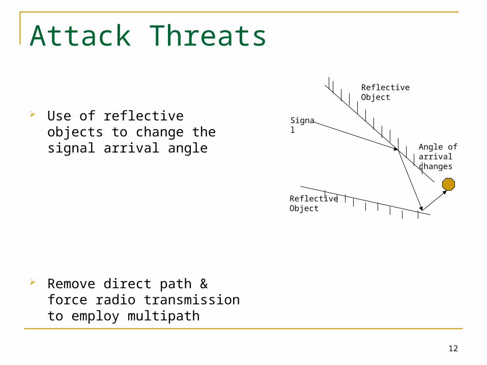
Attack Threats
Use of reflective objects to change the signal arrival angle
Remove direct path & force radio transmission to employ multipath
Reflective Object
Reflective Object
Signal
Angle of arrival changes

13
Related Work
DV – Hop
Three stages – Calculate distance in hops to anchor nodes (using beacons)
An anchor node calculates distance to other anchor nodes
Correction (average per hop distance) is calculated for each anchor node and deployed to the nodes
i ≠ j – for all anchor nodes j
i
jiji
i h
YYXXc
22

14
DV Hop
Example

15
Attack Threats
Vary hop count:
Wormhole
Jamming
Varying the radio range
Vary the per-hop distance

16
Attack Threats
Wormhole and Jamming

17
Related Work APIT (Approximate Point-in-Triangulation
Test)
Uses area-based (Region Inclusion) estimation
Environment divided into triangular regions
PIT test narrows the location of the node
Calculated the Center of Gravity of the narrowed region

18
Attack Threats
Alter neighborhood
Wormholes
Jamming
Changing the shape of the received radio region Placing an absorbing barrier
Alter the per-hop measurement

19
Least Squares
According to Wikipedia, is used to model the numerical data obtained from observations by adjusting the parameters of the model so as to get an optimal fit for the data.
Optimal fit – Sum of squared residuals having least value
Residue – Difference between the observed value and the value given by the model
Has its own shortcomings, which we will see soon

20
Localization Schemes
Triangulation & Trilateration
Collecting (x, y, d) values for each node
(x, y) coordinates of the anchor node
d is the distance to the anchor node
Using sufficient (xi, yi, di) solving for (x0, y0) is a simple least squares problem
)1.........(..........)()(),( 20
20
2 yyxxyxd
da
db dc
(Xa, ya)
(Xc, yc)(Xb, yb)
(x0, y0)

21
Shortcomings of Least Squares Non-robustness to outliers
A single incorrect (x, y, d) value may deviate the location estimate significantly away from the true value in spite of other correct values being present
e.g. altering hop count using wormhole or jamming attacks may deviate d significantly from its original value
Let 10 samples values of ‘d’ be – 8, 9, 10, 11, 8, 9, 10, 11, 9, 10;
However if an attacker changes one ’10’ to ‘100’, it will significantly affect the location measurement

22
Robust Fitting: Least Median of Squares Fitting: Finding the best fitting curve for a given set of points Cost Function for LS algorithm (in this case) is given by:
where d is the parameter to be estimated (distance), is the i-th measured distance, xi and yi are the coordinates of the i-th location and x0 and y0 are the coordinates of the true location
A single outlier may ruin the estimation due to the summation in the cost function
N
iiii yyxxddJ
1
220
20
' ][)(
'id

23
Robust Localization with Least Median of Squares Under ideal conditions (no attacks), the device location can be
estimated by …..(A)
value of the argument for which the value of the expression attains its minimum value
In presence of adversaries, we get outliers. Instead of trying to identify the outliers, we want to live with the bad nodes. This is achieved using LMS instead of LS
….(B)
N
iiii
yxdyyxxyx
1
220
20
),(00 ])()([minarg)ˆ,ˆ(
00
220
20
),(00 ])()([minarg)ˆ,ˆ(
00iiii
yxdyyxxmedyx

24
Non-linear and Linear Least Squares Equation A is a nonlinear least squares problem and is equivalent to
solving:
Averaging the left and right sides:

25
Non-linear and Linear Least Squares Subtracting the last two equations …
which is a linear LS problem

26
Non-linear and Linear Least Squares Linear LS has less computational complexity
Starting with a linear estimate can avoid local minimum
Linear LS and nonlinear LS starting from the linear estimate

27
Simulation – Threat Model Contamination Ratio Є < 50%, the fraction of distance measurements
compromised
Coordinated corruption of data rather than random perturbations
Adversary tries to modify NЄ values so that they all “vote” for (xa, ya)
(xa, ya)
(x0,y0)
Greater the da, stronger is the attack
202
0 yyxxd aaa
da

28
Simulation Linear LS used
mean square error of an estimator (quantity to be measured), according to wikipedia is:
In simple words, it is the estimation error, i.e. how much the experimental value differs from the mathematical value
Experiments conducted with different contamination ratio Є and measurement noise level
Implemented system robust to 30 percent contamination
n

29
Results
Each point represents average over 2000 trials

30
Results Impacts of Є and :
Severe performance degradation observed at Є = .35
n

31
Switched LS-LMS Localization Scheme
For 50 samples: x = 31… 50 represents outliers y represents values

32
Switched LS-LMS Localization Scheme Inliers and outliers well separated – LMS performs good
Inliers and outliers pretty close, LMS cannot differentiate and messes up – fits partly inlier and partly outlier data giving a worse estimate
A threshold T is selected and is compared with where is the observed noise level and normal measurement noise level is known
If T < LMS is used, else LS
nn
n
n
n
n

33
Results

34
RF-Based Fingerprinting Multiple anchor points deployed
Signal strengths at each anchor point recorded as {x, y, ss1,…ssN} where ss are the corresponding signal strengths; x,y is the position, N is number of anchor nodes (at least 3)
Beacons are broadcasted and signal strengths measured at each anchor node
The signal strengths ss’ (observed) are compared with the ones recorded by the central anchor node
The closest match is selected as the estimated location (minimum value of )

35
Robust Methods for RF-Based Fingerprinting A single corrupted signal strength at an anchor node will affect the
location. This can be easily done by: Using an absorbing barrier between the node and anchor node
Turning a microwave on
Instead of finding minimized Euclidean distance we can find the minimized median - to find the location

36
Conclusions Finding a correct estimate of the location is important
Adversaries will always be there, so live in harmony – rather than trying to eliminate all the attacks, tolerate them
Both LS and LMS have their pros and cons
Switched LS-LMS does the trick!
Median based distance metric is good for RF based fingerprinting

37
Limitations
LS-LMS scheme fails when the contamination ratio increases more than 50%
For large number of compromised nodes, median may be far different from the average value

38
Future Work
Limited attacker capabilities considered. That is, the attacker can compromise only a limited number of percentage of nodes.
Errors caused by malicious users considered. They have not considered errors caused due to limitations of ranging methods like signal attenuation, multipath signals, etc.

39
Thank You !!