1 Robust distributed linear programming - arXiv · 1 Robust distributed linear programming Dean...

arX

iv:1

409.

7140

v1 [

mat

h.O

C]

25 S

ep 2

014

1

Robust distributed linear programming

Dean Richert Jorge Cortes

Abstract

This paper presents a robust, distributed algorithm to solve general linear programs. The algorithm

design builds on the characterization of the solutions of the linear program as saddle points of a modified

Lagrangian function. We show that the resulting continuous-time saddle-point algorithm is provably

correct but, in general, not distributed because of a globalparameter associated with the nonsmooth exact

penalty function employed to encode the inequality constraints of the linear program. This motivates the

design of a discontinuous saddle-point dynamics that, while enjoying the same convergence guarantees,

is fully distributed and scalable with the dimension of the solution vector. We also characterize the

robustness against disturbances and link failures of the proposed dynamics. Specifically, we show that

it is integral-input-to-state stable but not input-to-state stable. The latter fact is a consequence of a more

general result, that we also establish, which states that noalgorithmic solution for linear programming

is input-to-state stable when uncertainty in the problem data affects the dynamics as a disturbance. Our

results allow us to establish the resilience of the proposeddistributed dynamics to disturbances of finite

variation and recurrently disconnected communication among the agents. Simulations in an optimal

control application illustrate the results.

I. INTRODUCTION

Linear optimization problems, or simply linear programs, model a broad array of engineering

and economic problems and find numerous applications in diverse areas such as operations

research, network flow, robust control, microeconomics, and company management. In this paper,

we are interested in both the synthesis of distributed algorithms that can solve standard form linear

programs and the characterization of their robustness properties. Our interest is motivated by

multi-agent scenarios that give rise to linear programs with an intrinsic distributed nature. In such

contexts, distributed approaches have the potential to offer inherent advantages over centralized

Incomplete versions of this paper were submitted to the 2013American Control Conference and the 2013 IEEE Conference

on Decision and Control.

The authors are with the Department of Mechanical and Aerospace Engineering, University of California, San Diego, CA

92093, USA,drichert,[email protected]

September 26, 2014 DRAFT

http://arxiv.org/abs/1409.7140v1

2

solvers. Among these, we highlight the reduction on communication and computational overhead,

the availability of simple computation tasks that can be performed by inexpensive and low-

performance processors, and the robustness and adaptive behavior against individual failures.

Here, we consider scenarios where individual agents interact with their neighbors and are only

responsible for computing their own component of the solution vector of the linear program. We

study the synthesis of provably correct, distributed algorithms that make the aggregate of the

agents’ states converge to a solution of the linear program and are robust to disturbances and

communication link failures.

Literature review.Linear programs play an important role in a wide variety of applications,

including perimeter patrolling [1], task allocation [2], [3], operator placement [4], process con-

trol [5], routing in communication networks [6], and portfolio optimization [7]. This relevance

has historically driven the design of efficient methods to solve linear optimization problems, see

e.g., [8], [9], [10]. More recently, the interest on networked systems and multi-agent coordination

has stimulated the synthesis of distributed strategies to solve linear programs [11], [12], [13] and

more general optimization problems with constraints, see e.g., [14], [15], [16] and references

therein. The aforementioned works build on consensus-based dynamics [17], [18], [19], [20]

whereby individual agents agree on the global solution to the optimization problem. This is a

major difference with respect to our work here, in which eachindividual agent computes only its

own component of the solution vector by communicating with its neighbors. This feature makes

the messages transmitted over the network independent of the size of the solution vector, and

hence scalable (a property which would not be shared by a consensus-based distributed optimiza-

tion method for the particular class of problems consideredhere). Some algorithms that enjoy a

similar scalability property exist in the literature. In particular, the recent work [21] introduces

a partition-based dual decomposition algorithm for network optimization. Other discrete-time

algorithms for non-strict convex problems are proposed in [22], [23], but require at least one of

the exact solutions of a local optimization problem at each iteration, bounded feasibility sets, or

auxiliary variables that increase the problem dimension. The algorithm in [24] on the other hand

only achieves convergence to an approximate solution of theoptimization problem. Closer to our

approach, although without equality constraints, the works [25], [26] build on the saddle-point

dynamics of a smooth Lagrangian function to propose algorithms for linear programming. The

resulting dynamics are discontinuous because of the projections taken to keep the evolution within

the feasible set. Both works establish convergence in the primal variables under the assumption


3

that the solution of the linear program is unique [26] or thatSlater’s condition is satisfied [25],

but do not characterize the properties of the final convergence point in the dual variables, which

might indeed not be a solution of the dual problem. We are unaware of works that explicitly

address the problem of studying the robustness of linear programming algorithms, particularly

from a systems and control perspective. This brings up another point of connection of the present

treatment with the literature, which is the body of work on robustness of dynamical systems

against disturbances. In particular, we explore the properties of our proposed dynamics with

respect to notions such as robust asymptotic stability [27], input-to-state stability (ISS) [28], and

integral input-to-state stability (iISS) [29]. The term ‘robust optimization’ often employed in the

literature, see e.g. [30], refers instead to worst-case optimization problems where uncertainty in

the data is explicitly included in the problem formulation.In this context, ‘robust’ refers to the

problem formulation and not to the actual algorithm employed to solve the optimization.

Statement of contributions.We consider standard form linear programs, which contain both

equality and non-negativity constraints on the decision vector. Our first contribution is an al-

ternative formulation of the primal-dual solutions of the linear program as saddle points of a

modified Lagrangian function. This function incorporates an exact nonsmooth penalty function to

enforce the inequality constraints. Our second contribution concerns the design of a continuous-

time dynamics that find the solutions of standard form linearprograms. Our alternative problem

formulation motivates the study of the saddle-point dynamics (gradient descent in one variable,

gradient ascent in the other) associated with the modified Lagrangian. It should be noted that,

in general, saddle points are only guaranteed to be stable (and not necessarily asymptotically

stable) for the corresponding saddle-point dynamics. Nevertheless, in our case, we are able

to establish the global asymptotic stability of the (possibly unbounded) set of primal-dual

solutions of the linear program and, moreover, the pointwise convergence of the trajectories.

Our analysis relies on the set-valued LaSalle Invariance Principle and, in particular, a careful

use of the properties of weakly and strongly invariant sets of the saddle-point dynamics. In

general, knowledge of the global parameter associated withthe nonsmooth exact penalty function

employed to encode the inequality constraints is necessaryfor the implementation of the saddle-

point dynamics. To circumvent this need, we propose an alternative discontinuous saddle-point

dynamics that does not require such knowledge and is fully distributed over a multi-agent system

in which each individual computes only its own component of the solution vector. We show that

the discontinuous dynamics share the same convergence properties of the regular saddle-point


4

dynamics by establishing that, for sufficiently large values of the global parameter, the trajectories

of the former are also trajectories of the latter. Two key advantages of our methodology are that

it (i) allows us to establish global asymptotic stability ofthe discontinuous dynamics without

establishing any regularity conditions on the switching behavior and (ii) sets the stage for the

characterization of novel and relevant algorithm robustness properties. This latter point bring

us to our third contribution, which pertains the robustnessof the discontinuous saddle-point

dynamics against disturbances and link failures. We establish that no continuous-time algorithm

that solves general linear programs can be input-to-state stable (ISS) when uncertainty in the

problem data affects the dynamics as a disturbance. As our technical approach shows, this fact

is due to the intrinsic properties of the primal-dual solutions to linear programs. Nevertheless,

when the set of primal-dual solutions is compact, we show that our discontinuous saddle-

point dynamics possesses an ISS-like property against small constant disturbances and, more

importantly, is integral input-to-state stable (iISS) – and thus robust to finite energy disturbances.

Our proof method is based on identifying a suitable iISS Lyapunov function, which we build

by combining the Lyapunov function used in our LaSalle argument and results from converse

Lyapunov theory. We conclude that one cannot expect better disturbance rejection properties

from a linear programming algorithm than those we establishfor our discontinuous saddle-point

dynamics. These results allow us to establish the robustness of our dynamics against disturbances

of finite variation and communication failures among agentsmodeled by recurrently connected

graphs. Simulations in an optimal control problem illustrate the results.

Organization.Section II introduces basic preliminaries. Section III presents the problem state-

ment. Section IV proposes the discontinuous saddle-point dynamics, establishes its convergence,

and discusses its distributed implementation. Sections V and VI study the algorithm robustness

against disturbances and communication link failures, respectively. Simulations illustrate our

results in Section VII. Finally, Section VIII summarizes our results and ideas for future work.

II. PRELIMINARIES

Here, we introduce notation and basic notions on nonsmooth analysis and dynamical systems.

This section may be safely skipped by the reader who is familiar with the notions reviewed here.

A. Notation and basic notions

The set of real numbers isR. Forx ∈ Rn, x ≥ 0 (resp.x > 0) means that all components ofx

are nonnegative (resp. positive). Forx ∈ Rn, we definemax0, x = (max0, x1, . . . ,max0, xn) ∈


5

Rn≥0. We let 1n ∈ R

n denote the vector of ones. We use‖ · ‖ and ‖ · ‖∞ to denote the2- and

∞-norms inRn. The Euclidean distance from a pointx ∈ Rn to a setA ⊂ R

n is denoted by

‖ · ‖A. The setB(x, δ) ⊂ Rn is the open ball centered atx ∈ R

n with radiusδ > 0. The set

A ⊂ Rn is convex if it fully contains the segment connecting any twopoints inA.

A function V : Rn → R is positive definite with respect toA ⊂ Rn if (i) V (x) = 0 for all

x ∈ A andV (x) > 0 for all x /∈ A. If A = 0, we refer toV as positive definite.V : Rn → R

is radially unbounded with respect toA if V (x) → ∞ when‖x‖A → ∞. If A = 0, we refer to

V as radially unbounded. A functionV is proper with respect toA if it is both positive definite

and radially unbounded with respect toA. A set-valued mapF : Rn⇒ R

n maps elements in

Rn to subsets ofRn. A function V : X → R defined on the convex setX ⊂ R

n is convex

if V (kx + (1 − k)y) ≤ kV (x) + (1 − k)V (y) for all x, y ∈ X and k ∈ [0, 1]. V is concave

iff −V is convex. Givenρ ∈ R, we defineV −1(≤ ρ) = x ∈ X | V (x) ≤ ρ. The function

L : X × Y → R defined on the convex setX × Y ⊂ Rn ×R

m is convex-concave if it is convex

on its first argument and concave on its second. A point(x, y) ∈ X × Y is a saddle point ofL

if L(x, y) ≥ L(x, y) ≥ L(x, y) for all (x, y) ∈ X × Y .

The notion of comparison function is useful to formalize stability properties. The class of

K functions is composed by functions of the form[0,∞) → [0,∞) that are continuous, zero

at zero, and strictly increasing. The subset of classK functions that are unbounded are called

classK∞. A classKL function [0,∞) × [0,∞) → [0,∞) is classK in its first argument and

continuous, decreasing, and converging to zero in its second argument.

An undirected graph is a pairG = (V, E), whereV = 1, . . . , n is a set of vertices and

E ⊆ V ×V is a set of edges. Given a matrixA ∈ Rm×n, we call a graphconnected with respect

to A if for each ℓ ∈ 1, . . . , m such thataℓ,i 6= 0 6= aℓ,j, it holds that(i, j) ∈ E .

B. Nonsmooth analysis

Here we review some basic notions from nonsmooth analysis following [31]. A function

V : Rn → R is locally Lipschitz atx ∈ R

n if there existδx > 0 and Lx ≥ 0 such that

|V (y1)−V (y2)| ≤ Lx‖y1− y2‖ for y1, y2 ∈ B(x, δx). If V is locally Lipschitz at allx ∈ Rn, we

refer toV as locally Lipschitz. IfV is convex, then it is locally Lipschitz. A locally Lipschitz

function is differentiable almost everywhere. LetΩV ⊂ Rn be then the set of points whereV is

not differentiable. The generalized gradient of a locally Lipschitz functionV at x ∈ Rn is

∂V (x) = co

limi→∞

∇V (xi) : xi → x, xi /∈ S ∪ ΩV

,


6

where co· denotes the convex hull andS ⊂ Rn is any set with zero Lebesgue measure.

A critical point x ∈ Rn of V satisfies0 ∈ ∂V (x). For a convex functionV , the first-order

condition of convexity states thatV (y) ≥ V (x) + (y − x)Tg for all g ∈ ∂V (x) andx, y ∈ Rn.

For V : Rn × Rn → R and (x, y) ∈ R

n × Rn, we use∂xV (x, y) and ∂yV (x, y) to denote the

generalized gradients of the mapsx′ 7→ V (x′, y) at x andy′ 7→ V (x, y′) at y, respectively.

A set-valued mapF : X ⊂ Rn⇒ R

n is upper semi-continuous if for allx ∈ X andε ∈ (0,∞)

there existsδx ∈ (0,∞) such thatF (y) ⊆ F (x) + B(0, ε) for all y ∈ B(x, δx). Conversely,F is

lower semi-continuous if for allx ∈ X, ε ∈ (0,∞), and any open setA intersectingF (x) there

exists aδ ∈ (0,∞) such thatF (y) intersectsA for all y ∈ B(x, δ). If F is both upper and lower

semi-continuous then it is continuous. Also,F is locally bounded if for everyx ∈ X there exist

ε ∈ (0,∞) andM > 0 such that‖z‖ ≤ M for all z ∈ F (y) and ally ∈ B(x, ε).

Lemma II.1 (Properties of the generalized gradient).If V : Rn → R is locally Lipschitz

at x ∈ Rn, then ∂V (x) is nonempty, convex, and compact. Moreover,x 7→ ∂V (x) is locally

bounded and upper semi-continuous.

C. Set-valued dynamical systems

Our exposition on basic concepts for set-valued dynamical systems follows [32]. A time-

invariant set-valued dynamical system is represented by the differential inclusion

x ∈ F (x), (1)

where t ∈ R≥0 andF : Rn⇒ R

n is a set valued map. IfF is locally bounded, upper semi-

continuous and takes nonempty, convex, and compact values,then from any initial condition

in Rn, there exists an absolutely continuous curvex : R≥0 → R

n, called solution, satisfying (1)

almost everywhere. The solution is maximal if it cannot be extended forward in time. The set

of equilibria of F is defined asx ∈ Rn | 0 ∈ F (x). A set M is strongly (resp. weakly)

invariant with respect to (1) if, for eachx0 ∈ M, M contains all (resp. at least one) maximal

solution(s) of (1) with initial conditionx0. The set-valued Lie derivative of a differentiable

function V : Rn → R along the trajectories of (1) is defined as

LFV (x) = ∇V (x)T v : v ∈ F (x).

The following result helps establish the asymptotic convergence properties of (1).


7

Theorem II.2 (Set-valued LaSalle Invariance Principle).LetX ⊂ Rn be compact and strongly

invariant with respect to(1). AssumeV : Rn → R is differentiable andF is locally bounded,

upper semi-continuous and takes nonempty, convex, and compact values. IfLFV (x) ⊂ (−∞, 0]

for all x ∈ X, then any solution of(1) starting inX converges to the largest weakly invariant

setM contained inx ∈ X : 0 ∈ LFV (x).

Differential inclusions are specially useful to handle differential equations with discontinuities.

Specifically, letf : X ⊂ Rn → R

n be a piecewise continuous vector field and consider

x = f(x). (2)

The classical notion of solution is not applicable to (2) because of the discontinuities. Instead,

consider the Filippov set-valued map associated tof , defined byF [f ](x) := co

limi→∞ f(xi) :

xi → x, xi /∈ Ωf

, whereco· denotes the closed convex hull andΩf are the points wheref

is discontinuous. One can show that the set-valued mapF [f ] is locally bounded, upper semi-

continuous and takes nonempty, convex, and compact values,and hence solutions exist to

x ∈ F [f ](x) (3)

starting from any initial condition. The solutions of (2) inthe sense of Filippov are, by definition,

the solutions of the differential inclusion (3).

III. PROBLEM STATEMENT AND EQUIVALENT FORMULATION

This section introduces standard form linear programs and describes an alternative formulation

that is useful later in fulfilling our main objective, which is the design of robust, distributed

algorithms to solve them. Consider the following standard form linear program,

min cTx (4a)

s.t. Ax = b, x ≥ 0, (4b)

wherex, c ∈ Rn, A ∈ R

m×n, andb ∈ Rm. We only consider feasible linear programs with finite

optimal value. The set of solutions to (4) is denoted byX ⊂ Rn. The dual formulation is

max − bT z (5a)

s.t. AT z + c ≥ 0. (5b)


8

The set of solutions to (5) is denoted byZ ⊂ Rm. We usex∗ andz∗ to denote a solution of (4)

and (5), respectively. The following result is a fundamental relationship between primal and dual

solutions of linear programs and can be found in many optimization references, see e.g., [10].

Theorem III.1 (Complementary slackness and strong duality). Suppose thatx ∈ Rn is

feasible for(4) and z ∈ Rm is feasible for(5). Thenx is a solution to(4) and z is a solution

to (5) if and only if (AT z + c)Tx = 0. In compact form,

X × Z = (x, z) ∈ Rn × R

m | Ax = b, x ≥ 0, AT z + c ≥ 0, (AT z + c)Tx = 0. (6)

Moreover, for any(x∗, z∗) ∈ X × Z, it holds thatcTx∗ = −bT z∗.

The equality(AT z + c)Tx = 0 is called thecomplementary slacknesscondition whereas

the property thatcTx∗ = −bT z∗ is called strong duality. One remarkable consequence of

Theorem III.1 is that the set on the right-hand side of (6) is convex (becauseX ×Z is convex).

This fact is not obvious since the complementary slackness condition is not affine in the variables

x andz. This observation will allow us to use a simplified version ofDanskin’s Theorem (see

Lemma A.2) in the proof of a key result of Section V. The next result establishes the connection

between the solutions of (4) and (5) and the saddle points of amodified Lagrangian function. Its

proof can be deduced from results on penalty functions that appear in optimization, see e.g. [33],

but we include it here for completeness and consistency of the presentation.

Proposition III.2 (Solutions of linear program as saddle points). For K ≥ 0, let LK :

Rn × R

m → R be defined by

LK(x, z) = cTx+1

2(Ax− b)T (Ax− b) + zT (Ax− b) +K1

Tn max0,−x. (7)

Then,LK is convex inx and concave (in fact, linear) inz. Moreover,

(i) if x∗ ∈ Rn is a solution of(4) and z∗ ∈ R

m is a solution of(5), then the point(x∗, z∗) is

a saddle point ofLK for anyK ≥ ‖AT z∗ + c‖∞,

(ii) if (x, z) ∈ Rn × R

m is a saddle point ofLK with K > ‖AT z∗ + c‖∞ for somez∗ ∈ Rm

solution of (5), then x ∈ Rn is a solution of (4).

Proof: One can readily see from (7) thatLK is a convex-concave function. Letx∗ be a

solution of (4) and letz∗ be a solution of (5). To show (i), using the characterizationof X ×Z


9

described in Theorem III.1 and the fact thatK ≥ ‖AT z∗ + c‖∞, we can write for anyx ∈ Rn,

LK(x, z∗) = cTx+ (Ax− b)T (Ax− b) + zT∗ (Ax− b) +K1

Tn max0,−x,

≥ cTx+ zT∗ (Ax− b) + (AT z∗ + c)T max0,−x,

≥ cTx+ zT∗ (Ax− b)− (AT z∗ + c)Tx,

= cTx+ zT∗ A(x− x∗)− (AT z∗ + c)T (x− x∗),

= cTx− cT (x− x∗) = cTx∗ = LK(x∗, z∗).

The fact thatLK(x∗, z) = LK(x∗, z∗) for any z ∈ Rm is immediate. These two facts together

imply that (x∗, z∗) is a saddle point ofLK .

We prove (ii) by contradiction. Let(x, z) be a saddle point ofLK with K > ‖AT z∗+ c‖∞ for

somez∗ ∈ Z, but supposex is not a solution of (4). Letx∗ ∈ X . Since for fixedx, z 7→ LK(x, z)

is concave and differentiable, a necessary condition for(x, z) to be a saddle point ofLK is that

Ax− b = 0. Using this fact,LK(x∗, z) ≥ LK(x, z) can be expressed as

cTx∗ ≥ cT x+K1

Tn max0,−x. (8)

Now, if x ≥ 0, thencTx∗ ≥ cT x, and thusx would be a solution of (4). If, instead,x 6≥ 0,

cT x = cTx∗ + cT (x− x∗),

= cTx∗ − zT∗ A(x− x∗) + (AT z∗ + c)T (x− x∗),

= cTx∗ − zT∗ (Ax− b) + (AT z∗ + c)T x,

> cTx∗ −K1

Tn max0,−x,

which contradicts (8), concluding the proof.

The relevance of Proposition III.2 is two-fold. On the one hand, it justifies searching for the

saddle points ofLK instead of directly solving the constrained optimization problem (4). On

the other hand, given thatLK is convex-concave, a natural approach to find the saddle points

is via the associated saddle-point dynamics. However, for an arbitrary function, such dynamics

is known to render saddle points only stable, not asymptotically stable (in fact, the saddle-

point dynamics derived using the standard Lagrangian for a linear program does not converge

to a solution of the linear program, see e.g., [34], [26]). Interestingly [26], the convergence

properties of saddle-point dynamics can be improved using penalty functions associated with

the constraints to augment the cost function. In our case, weaugment the linear cost function


10

cTx with a quadratic penalty for the equality constraints and a nonsmooth penalty function for

the inequality constraints. This results in the nonlinear optimization problem,

minAx=b

cTx+ ‖Ax− b‖2 +K1

Tn max0,−x,

whose standard Lagrangian is equivalent toLK . We use the nonsmooth penalty function to

ensure that there is anexactequivalence between saddle points ofLK and the solutions of (4).

Instead, the use of smooth penalty functions such as the logarithmic barrier function used in [16],

results only in approximate solutions. In the next section,we show that indeed the saddle-point

dynamics ofLK asymptotically converges to saddle points.

Remark III.3 (Bounds on the parameter K). It is worth noticing that the lower bounds

on K in Proposition III.2 are characterized by certain dual solutions, which are unknown a

priori. Nevertheless, our discussion later shows that thisproblem can be circumvented and that

knowledge of such bounds is not necessary for the design of robust, distributed algorithms that

solve linear programs. •

IV. SADDLE-POINT DYNAMICS FOR DISTRIBUTED LINEAR PROGRAMMING

In this section, we design a continuous-time algorithm to find the solutions of (4) and discuss its

distributed implementation in a multi-agent system. We further build on the elements of analysis

introduced here to characterize the robustness propertiesof linear programming dynamics in

the forthcoming sections. Building on the result in Proposition III.2, we consider the saddle-

point dynamics (gradient descent in one argument, gradientascent in the other) of the modified

LagrangianLK . Our presentation proceeds by characterizing the properties of this dynamics and

observing its limitations, leading up to the main contribution, which is the introduction of a

discontinuous saddle-point dynamics amenable to distributed implementation.

The nonsmooth character ofLK means that its saddle-point dynamics takes the form of the

following differential inclusion,

x+ c+ AT (z + Ax− b) ∈ −K∂max0,−x, (9a)

z = Ax− b. (9b)

For notational convenience, we useFKsdl : R

n × Rm⇒ R

n × Rm to denote the set-valued vector

field which defines the differential inclusion (9). The following result characterizes the asymptotic

convergence of (9) to the set of solutions to (4)-(5).


11

Theorem IV.1 (Asymptotic convergence to the primal-dual solution set). Let (x∗, z∗) ∈ X×Z

and defineV : Rn × Rm → R≥0 as

V (x, z) =1

2(x− x∗)

T (x− x∗) +1

2(z − z∗)

T (z − z∗).

For ∞ > K ≥ ‖AT z∗+ c‖∞, it holds thatLFKsdlV (x, z) ⊂ (−∞, 0] for all (x, z) ∈ R

n×Rm and

any trajectoryt 7→ (x(t), z(t)) of (9) converges asymptotically to the setX × Z.

Proof: Our proof strategy is based on verifying the hypotheses of the LaSalle Invariance

Principle, cf. Theorem II.2, and identifying the set of primal-dual solutions as the corresponding

largest weakly invariant set. First, note that Lemma II.1 implies thatFKsdl is locally bounded,

upper semi-continuous and takes nonempty, convex, and compact values. By Proposition III.2(i),

(x∗, z∗) is a saddle point ofLK whenK ≥ ‖AT z∗ + c‖∞. Consider the quadratic functionV

defined in the theorem statement, which is continuously differentiable and radially unbounded.

Let a ∈ LFKsdlV (x, z). By definition, there existsv =(−c−AT (z+Ax−b)−gx, Ax−b) ∈ FK

sdl(x, z),

with gx ∈ K∂max0,−x, such that

a = vT∇V (x, z) = (x−x∗)T (−c−AT (z+Ax−b)−gx)+(z − z∗)(Ax− b). (10)

SinceLK is convex in its first argument, andc+AT (z +Ax− b) + gx ∈ ∂xLK(x, z), using the

first-order condition of convexity, we have

LK(x, z) ≤ LK(x∗, z)+(x−x∗)T(

c+AT (z+Ax−b)+gx)

.

SinceLK is linear inz, we haveLK(x, z) = LK(x, z∗) + (z − z∗)T (Ax− b). Using these facts

in (10), we get

a ≤ LK(x∗, z)− LK(x, z∗) = LK(x∗, z)− LK(x∗, z∗) + LK(x∗, z∗)− LK(x, z∗) ≤ 0,

since(x∗, z∗) is a saddle point ofLK . Sincea is arbitrary, we deduce thatLFKsdlV (x, z) ⊂ (−∞, 0].

For any givenρ ≥ 0, this implies that the sublevel setV −1(≤ ρ) is strongly invariant with respect

to (9). SinceV is radially unbounded,V −1(≤ ρ) is also compact. The conditions of Theorem II.2

are then satisfied withX = V −1(≤ ρ), and therefore any trajectory of (9) starting inV −1(≤ ρ)

converges to the largest weakly invariant setM in (x, z) ∈ V −1(≤ ρ) : 0 ∈ LFKsdlV (x, z)

(note that for any initial condition(x0, z0) one can choose aρ such that(x0, z0) ∈ V −1(≤ ρ)).

This set is closed, which can be justified as follows. SinceFKsdl is upper semi-continuous and

V is continuously differentiable, the map(x, z) 7→ LFKsdlV (x, z) is also upper semi-continuous.


12

Closedness then follows from [35, Convergence Theorem]. Wenow show thatM ⊆ X ×Z. To

start, take(x′, z′) ∈ M. ThenLK(x∗, z∗)− LK(x′, z∗) = 0, which implies

LK(x′, z∗)− (Ax′ − b)T (Ax′ − b) = 0, (11)

whereLK(x′, z∗) = cTx∗ − cTx′ − zT∗ (Ax′ − b) −K1

Tn max0,−x′. Using strong duality, the

expression ofLK can be simplified toLK(x′, z∗) = −(AT z∗ + c)Tx′ − K1

Tn max0,−x′. In

addition,AT z∗+c ≥ 0 by dual feasibility. Thus, whenK ≥ ‖AT z∗+c‖∞, we haveLK(x, z∗) ≤ 0

for all (x, z) ∈ V −1(≤ ρ). This implies that(Ax′ − b)T (Ax′ − b) = 0 for (11) to be true, which

further implies thatAx′ − b = 0. Moreover, from the definition ofLK and the bound onK, one

can see that ifx′ 6≥ 0, thenLK(x′, z∗) < 0. Therefore, for (11) to be true, it must be thatx′ ≥ 0.

Finally, from (11), we get thatLK(x′, z∗) = cTx∗ − cTx′ = 0. In summary, if(x′, z′) ∈ M then

cTx∗ = cTx′, Ax′ − b = 0, andx′ ≥ 0. Therefore,x′ is a solution of (4). Now, we show that

z′ is a solution of (5). BecauseM is weakly invariant, there exists a trajectory starting from

(x′, z′) that remains inM. The fact thatAx′ = b implies that z = 0, and hencez(t) = z′ is

constant. For any giveni ∈ 1, . . . , n, we consider the cases (i)x′i > 0 and (ii) x′

i = 0. In

case (i), the dynamics of theith component ofx is xi = −(c + AT z′)i where (c + AT z′)i is

constant. It cannot be that−(c+AT z′)i > 0 because this would contradict the fact thatt 7→ xi(t)

is bounded. Therefore,(c + AT z′)i ≥ 0. If xi = −(c + AT z′)i < 0, thenxi(t) will eventually

become zero, which we consider in case (ii). In fact, since the solution remains inM, without

loss of generality, we can assume that(x′, z′) is such that eitherx′i > 0 and (c+AT z′)i = 0 or

x′i = 0 for eachi ∈ 1, . . . , n. Consider now case (ii). Sincexi(t) must remain non-negative

in M, it must be thatxi(t) ≥ 0 when xi(t) = 0. That is, inM, we havexi(t) ≥ 0 when

xi(t) = 0 and xi(t) ≤ 0 whenxi(t) > 0. Therefore, for any trajectoryt 7→ xi(t) in M starting

at x′i = 0, the unique Filippov solution is thatxi(t) = 0 for all t ≥ 0. As a consequence,

(c+ AT z′)i ∈ [0, K] if x′i = 0. To summarize cases (i) and (ii), we have

• Ax′ = b andx′ ≥ 0 (primal feasibility),

• AT z′ + c ≥ 0 (dual feasibility),

• (AT z′ + c)i = 0 if x′i > 0 andx′

i = 0 if (AT z′ + c)i > 0 (complementary slackness),

which is sufficient to show thatz ∈ Z (cf. Theorem III.1). HenceM ⊆ X × Z. Since the

trajectories of (9) converge toM, this completes the proof.

Using a slightly more complicated lower bound on the parameter K, we are able to show

point-wise convergence of the saddle-point dynamics. We state this result next.


13

Corollary IV.2 (Point-wise convergence of saddle-point dynamics).Let ρ > 0. Then, with the

notation of Theorem IV.1, for

∞ > K ≥ max(x,z)∈(X×Z)∩V −1(≤ρ)

‖AT z + c‖∞, (12)

it holds that any trajectoryt 7→ (x(t), z(t)) of (9) starting inV −1(≤ ρ) converges asymptotically

to a point inX × Z.

Proof: If K satisfies (12), then in particularK ≥ ‖AT z∗+c‖∞. Thus,V −1(≤ ρ) is strongly

invariant under (9) sinceLFKsdlV (x, z) ⊂ (−∞, 0] for all (x, z) ∈ V −1(≤ ρ) (cf. Theorem IV.1).

Also, V −1(≤ ρ) is bounded becauseV is quadratic. Therefore, by the Bolzano-Weierstrass

theorem [36, Theorem 3.6], there exists a subsequence(x(tk), z(tk)) ∈ V −1(≤ρ) that converges

to a point(x, z) ∈ (X × Z) ∩ V −1(≤ ρ). Given ε > 0, let k∗ be such that‖(x(tk∗), z(tk∗)) −

(x, z)‖ ≤ ε. Consider the functionV (x, z) = 12(x − x)T (x − x) + 1

2(z − z)T (z − z). When

K satisfies (12), again it holds thatK ≥ ‖AT z + c‖∞. Applying Theorem IV.1 once again,

V −1(≤ ρ) is strongly invariant under (9). Consequently, fort ≥ tk∗, we have(x(t), z(t)) ∈

V −1(≤ V (x(tk∗), z(tk∗))) = B(

(x, z), ‖(x(tk∗), z(tk∗))− (x, z)‖)

⊂ B((x, z), ε). Sinceε can be

taken arbitrarily small, this implies that(x(t), z(t)) converges to the point(x, z) ∈ X × Z.

Remark IV.3 (Choice of parameter K). The bound (12) for the parameterK depends on (i)

the primal-dual solution setX × Z as well as (ii) the initial condition, since the result is only

valid when the dynamics start inV −1(≤ ρ). However, if the setX ×Z is compact, the parameter

K can be chosen independently of the initial condition since the maximization in (12) would be

well defined when taken over the whole setX × Z. We should point out that, in Section IV-A

we introduce a discontinuous version of the saddle-point dynamics which does not involveK.•

A. Discontinuous saddle-point dynamics

Here, we propose an alternative dynamics to (9) that does notrely on knowledge of the

parameterK and also converges to the solutions of (4)-(5). We begin by defining thenominal

flow functionfnom : Rn≥0 × R

m → Rn by

fnom(x, z) := −c− AT (z + Ax− b).


14

This definition is motivated by the fact that, for(x, z) ∈ Rn>0 × R

m, the set∂xLK(x, z) is the

singleton−fnom(x, z). The discontinuous saddle-point dynamicsis, for i ∈ 1, . . . , n,

xi =

fnomi (x, z), if xi > 0,

max0, fnomi (x, z), if xi = 0,

(13a)

z = Ax− b. (13b)

When convenient, we use the notationfdis : Rn≥0×R

m → Rn×R

m to refer to the discontinuous

dynamics (13). Note that the discontinuous function that defines the dynamics (13a) is simply

the positive projection operator, i.e., whenxi = 0, it corresponds to the projection offnomi (x, z)

onto R≥0. We understand the solutions of (13) in the Filippov sense. We begin our analysis

by establishing a relationship between the Filippov set-valued map offdis and the saddle-point

dynamicsFKsdl which allows us to relate the trajectories of (13) and (9).

Proposition IV.4 (Trajectories of the discontinuous saddle-point dynamics are trajectories

of the saddle-point dynamics).Let ρ > 0 and (x∗, z∗) ∈ X × Z be given and the functionV

be defined as in Theorem IV.1. Then, for any

∞ > K ≥ K1 := max(x,z)∈V −1(≤ρ)

‖fnom(x, z)‖∞,

the inclusionF [fdis](x, z) ⊆ FKsdl(x, z) holds for every(x, z) ∈ V −1(≤ ρ). Thus, the trajectories

of (13) starting in V −1(≤ ρ) are also trajectories of(9).

Proof: The projection onto theith component of the Filippov set-valued mapF [fdis] is

proji(F [fdis](x, z)) =

fnomi (x, z), if i ∈ 1, . . . , n andxi > 0,

[fnomi (x, z),max0, fnom

i (x, z)], if i ∈ 1, . . . , n andxi = 0,

(Ax− b)i, if i ∈ n+ 1, . . . , n+m.

As a consequence, for anyi ∈ n+ 1, . . . , n+m, we have

proji(FKsdl(x, z)) = (Ax− b)i = proji(F [fdis](x, z)),

and, for anyi ∈ 1, . . . , n such thatxi > 0, we have

proji(FKsdl(x, z)) = (−c− AT (Ax− b+ z))i = fnom

i (x, z) = proji(F [fdis](x, z)).


15

Thus, let us consider the case whenxi = 0 for somei ∈ 1, . . . , n. In this case, note that

proji(F [fdis](x, z)) = [fnomi (x, z),max0, fnom

i (x, z)] ⊆ [fnomi (x, z), fnom

i (x, z) + |fnomi (x, z)|],

proji(FKsdl(x, z)) = [fnom

i (x, z), fnomi (x, z) +K].

The choiceK ≥ |fnomi (x, z)| for eachi ∈ 1, . . . , n makesF [fdis](x, z) ⊆ FK

sdl(x, z). More

generally, sinceV −1(ρ) is compact andfnom is continuous, the choice

∞ > K ≥ max(x,z)∈V −1(ρ)

‖fnom(x, z)‖∞,

guaranteesF [fdis](x, z) ⊆ FKsdl(x, z) for all (x, z) ∈ V −1(ρ). By Theorem IV.1, we know thatV

is non-increasing along (9), implying thatV −1(≤ ρ) is strongly invariant with respect to (9), and

hence (13) too. Therefore, any trajectory of (13) starting in V −1(≤ ρ) is a trajectory of (9).

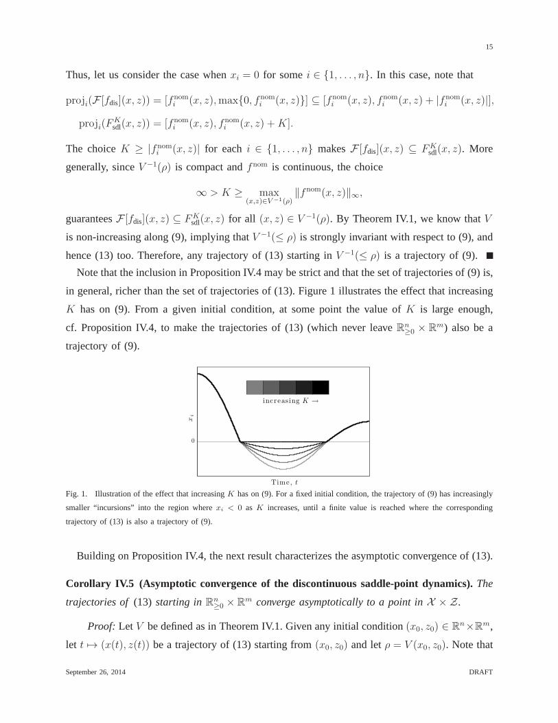
Note that the inclusion in Proposition IV.4 may be strict andthat the set of trajectories of (9) is,

in general, richer than the set of trajectories of (13). Figure 1 illustrates the effect that increasing

K has on (9). From a given initial condition, at some point the value ofK is large enough,

cf. Proposition IV.4, to make the trajectories of (13) (which never leaveRn≥0 × R

m) also be a

trajectory of (9).

0

xi

Time, t

increasing K →

Fig. 1. Illustration of the effect that increasingK has on (9). For a fixed initial condition, the trajectory of (9) has increasingly

smaller “incursions” into the region wherexi < 0 as K increases, until a finite value is reached where the corresponding

trajectory of (13) is also a trajectory of (9).

Building on Proposition IV.4, the next result characterizes the asymptotic convergence of (13).

Corollary IV.5 (Asymptotic convergence of the discontinuous saddle-point dynamics).The

trajectories of (13) starting inRn≥0 × R

m converge asymptotically to a point inX × Z.

Proof: Let V be defined as in Theorem IV.1. Given any initial condition(x0, z0) ∈ Rn×R

m,

let t 7→ (x(t), z(t)) be a trajectory of (13) starting from(x0, z0) and letρ = V (x0, z0). Note that


16

t 7→ (x(t), z(t)) does not depend onK because (13) does not depend onK. Proposition IV.4

establishes thatt 7→ (x(t), z(t)) is also a trajectory of (9) forK ≥ K1. Imposing the additional

condition that

∞ > K ≥ max

K1, max(x∗,z∗)∈(X×Z)∩V −1(≤ρ)

‖AT z∗ + c‖∞

,

Corollary IV.2 implies that the trajectories of (9) (and thus t 7→ (x(t), z(t)) converge asymptot-

ically to a point inX ×Z.

One can also approach the convergence analysis of (13) from aswitched systems perspective,

which would require checking that certain regularity conditions hold for the switching behavior

of the system. We have been able to circumvent this complexity by relying on the powerful

stability tools available for set-valued dynamics to analyze (9) and by relating its solutions with

those of (13). Moreover, the interpretation of the trajectories of (13) in the Filippov sense is

instrumental for our analysis in Section V where we study therobustness against disturbances

using powerful Lyapunov-like tools for differential inclusions.

Remark IV.6 (Comparison to existing dynamics for linear programming). Though a central

motivation for the development of our linear programming algorithm is the establishment of

various robustness properties which we study next, the dynamics (13) and associated convergence

results of this section are both novel and have distinct contributions. The work [26] builds on

the saddle-point dynamics of a smooth Lagrangian function to introduce an algorithm for linear

programming. Instead of exact penalty functions, this approach uses projections to keep the

evolution within the feasible set, resulting in a discontinuous dynamics in both the primal and dual

variables. The work [25] employs a similar approach to deal with non-strictly convex programs

under inequality constraints, where projection is used instead employed to keep nonnegative the

value of the dual variables. These works establish convergence in the primal variables ([26] under

the assumption that the solution of the linear program is unique, [25] under the assumption that

Slater’s condition is satisfied) to a solution of the linear program. In both cases, the dual variables

converge to some unknown point which might not be a solution to the dual problem. This is

to be contrasted with the convergence properties of the dynamics (13) stated in Corollary IV.5

which only require the linear program to be feasible with finite optimal value. •


17

B. Distributed implementation

An important advantage of the dynamics (13) over other linear programming methods is that it

is well-suited for distributed implementation. To make this statement precise, consider a scenario

where each component ofx ∈ Rn corresponds to an independent decision maker or agent and

the interconnection between the agents is modeled by an undirected graphG = (V, E). To see

under what conditions the dynamics (13) can be implemented by this multi-agent system, let us

express it component-wise. First, the nominal flow functionin (13a) for agenti ∈ 1, . . . , n is,

fnomi (x, z) = −ci −

m∑

ℓ=1

aℓ,i

[

zℓ +n

∑

k=1

aℓ,kxk − bℓ

]

= −ci −∑

ℓ : aℓ,i 6=0aℓ,i

[

zℓ +∑

k : aℓ,k 6=0aℓ,kxk − bℓ

]

,

and the dynamics (13b) for eachℓ ∈ 1, . . . , m is

zℓ =∑

i : aℓ,i 6=0aℓ,ixi − bℓ. (14)

According to these expressions, in order for agenti ∈ 1, . . . , n to be able to implement its

corresponding dynamics in (13a), it also needs access to certain components ofz (specifically,

those componentszℓ for which aℓ,i 6= 0), and therefore needs to implement their corresponding

dynamics (14). We say that the dynamics (13) isdistributed overG when the following holds

(D1) for eachi ∈ V, agenti knows

a) ci ∈ R,

b) everybℓ ∈ R for which aℓ,i 6= 0,

c) the non-zero elements of every row ofA for which theith component,aℓ,i, is non-zero,

(D2) agenti ∈ V has control over the variablexi ∈ R,

(D3) G is connected with respect toA, and

(D4) agents have access to the variables controlled by neighboring agents.

Note that (D3) guarantees that the agents that implement (14) for a particularℓ ∈ 1, . . . , m

are neighbors inG.

Remark IV.7 (Scalability of the nominal saddle-point dynamics). A different approach to

solve (4) is the following: reformulate the optimization problem as the constrained minimization

of a sum of convex functions all of the form1ncTx and use the algorithms developed in, for

instance, [14], [15], [11], [12], [16], for distributed convex optimization. However, in this case,

this approach would lead to agents storing and communicating with neighbors estimates of the

entire solution vector inRn, and hence would not scale well with the number of agents of the


18

network. In contrast, to execute the discontinuous saddle-point dynamics, agents only need to

store the component of the solution vector that they controland communicate it with neighbors.

Therefore, the dynamics scales well with respect to the number of agents in the network. •

V. ROBUSTNESS AGAINST DISTURBANCES

Here we explore the robustness properties of the discontinuous saddle-point dynamics (13)

against disturbances. Such disturbances may correspond tonoise, unmodeled dynamics, or in-

correct agent knowledge of the data defining the linear program. Note that the global asymptotic

stability ofX×Z under (13) characterized in Section IV naturally provides arobustness guarantee

on this dynamics: whenX × Z is compact, sufficiently small perturbations do not destroythe

global asymptotic stability of the equilibria, cf. [27]. Our objective here is to go beyond this

qualitative statement to obtain a more precise, quantitative description of robustness. To this

end, we consider the notions of input-to-state stability (ISS) and integral-input-to-state stability

(iISS). In Section V-A we show that, when the disturbances correspond to uncertainty in the

problem data, no dynamics for linear programming can be ISS.This motivates us to explore the

weaker notion of iISS. In Section V-B we show that (13) with additive disturbances is iISS.

Remark V.1 (Robust dynamics versus robust optimization).We make a note of the distinction

between the notion of algorithm robustness, which is what westudy here, and the term robust

(or worst-case) optimization, see e.g., [30]. The latter refers to a type of problem formulation

in which some notion of variability (which models uncertainty) is explicitly included in the

problem statement. Mathematically,

min cTx s.t. f(x, ω) ≤ 0, ∀ω ∈ Ω,

whereω is an uncertain parameter. Building on the observation thatone only has to consider the

worst-case values ofω, one can equivalently cast the optimization problem with constraints that

only depend onx, albeit at the cost of a loss of structure in the formulation.Another point of

connection with the present work is the body of research on stochastic approximation in discrete

optimization, where the optimization parameters are corrupted by disturbances, see e.g. [37].•

Without explicitly stating it from here on, we make the following assumption along the section:

(A) The solution sets to (4) and (5) are compact (i.e.,X × Z is compact).

The justification for this assumption is twofold. On the technical side, our study of the iISS

properties of (15) in Section V-B builds on a Converse Lyapunov Theorem [27] which requires


19

the equilibrium set to be compact (the question of whether the Converse Lyapunov Theorem

holds when the equilibrium set is not compact and the dynamics is discontinuous is an open

problem). On the practical side, one can add box-type constraints to (4), ensuring that (A) holds.

We now formalize the disturbance model considered in this section. Letw = (wx, wz) : R≥0 →

Rn × R

m be locally essentially bounded and enter the dynamics as follows,

xi =

fnomi (x, z) + (wx)i, if xi > 0,

max0, fnomi (x, z) + (wx)i, if xi = 0,

∀i ∈ 1, . . . , n, (15a)

z = Ax− b+ wz. (15b)

For notational purposes, we usefwdis : R

2(n+m) → Rn+m to denote (15). We exploit the fact that

fnom is affine to state that the additive disturbancew captures unmodeled dynamics, measurement

and computation noise, and any error in an agent’s knowledgeof the problem data (A, b andc).

For example, if agenti ∈ 1, . . . , n uses an estimateci of ci when computing its dynamics, this

can be modeled in (15) by considering(wx(t))i = ci − ci. To make precise the correspondence

between the disturbancew and uncertainties in the problem data, we provide the following

convergence result when the disturbance is constant.

Corollary V.2 (Convergence under constant disturbances).For constantw = (wx, wz) ∈

Rn × R

m, consider theperturbed linear program,

min (c− wx − ATwz)Tx (16a)

s.t. Ax = b− wz, x ≥ 0, (16b)

and, with a slight abuse in notation, letX (w)×Z(w) be its primal-dual solution set. Suppose

thatX (w)×Z(w) is nonempty. Then each trajectory of(15) starting inRn≥0×R

m with constant

disturbancew(t) = w = (wx, wz) converges asymptotically to a point inX (w)×Z(w).

Proof: Note that (15) with disturbancew corresponds to the undisturbed dynamics (13) for

the perturbed problem (16). SinceX (w)× Z(w) 6= ∅, Corollary IV.5 implies the result.

A. No dynamics for linear programming is input-to-state stable

The notion of input-to-state stability (ISS) is a natural starting point to study the robustness

of dynamical systems against disturbances. Informally, ifa dynamics is ISS, then bounded

disturbances give rise to bounded deviations from the equilibrium set. Here we show that any


20

dynamics that (i) solve any feasible linear program and (ii)where uncertainties in the problem

data (A, b, andc) enter as disturbances is not input-to-state stable (ISS).Our analysis relies on

the properties of the solution set of a linear program. To make our discussion precise, we begin

by recalling the definition of input-to-state stability.

Definition V.3 (Input-to-state stability [28]). The dynamics(15) is ISS with respect toX ×Z

if there existβ ∈ KL and γ ∈ K such that, for any trajectoryt 7→ (x(t), z(t)) of (15), one has

‖(x(t), z(t))‖X×Z ≤ β(‖(x(0), z(0)‖X×Z , t) + γ(‖w‖∞),

for all t ≥ 0. Here,‖w‖∞ := esssups≥0 ‖w(s)‖ is the essential supremum ofw(t).

Our method to show that no dynamics is ISS is constructive. Wefind a constant disturbance

such that the primal-dual solution set to some perturbed linear program is unbounded. Since any

point in this unbounded solution set is a stable equilibriumby assumption, this precludes the

possibility of the dynamics from being ISS. This argument ismade precise next.

Theorem V.4 (No dynamics for linear programming is ISS).Consider the generic dynamics

(x, z) = Φ(x, z, v) (17)

with disturbancet 7→ v(t). Assume uncertainties in the problem data are modeled byv. That is,

there exists a surjective functiong = (g1, g2) : Rn+m → R

n × Rm with g(0) = (0, 0) such that,

for v ∈ Rn+m, the primal-dual solution setX (v)× Z(v) of the linear program

min (c+ g1(v))Tx (18a)

s.t. Ax = b+ g2(v), x ≥ 0. (18b)

is the stable equilibrium set of(x, z) = Φ(x, z, v) wheneverX (v) × Z(v) 6= ∅. Then, the

dynamics(17) is not ISS with respect toX ×Z.

Proof: We divide the proof in two cases depending on whetherAx = b, x ≥ 0 is (i)

unbounded or (ii) bounded. In both cases, we design a constant disturbancev(t) = v such that

the equilibria of (17) contains points arbitrarily far awayfrom X × Z. This would imply that

the dynamics is not ISS. Consider case (i). SinceAx = b, x ≥ 0 is unbounded, convex,

and polyhedral, there exists a pointx ∈ Rn and directionνx ∈ R

n \ 0 such thatx + λνx ∈

bd(Ax = b, x ≥ 0) for all λ ≥ 0. Herebd(·) refers to the boundary of the set. Letη ∈ Rn be

such thatηTνx = 0 and x+ εη /∈ Ax = b, x ≥ 0 for any ε > 0 (geometrically,η is normal to


21

and points out ofAx = b, x ≥ 0 at x). Now that these quantities have been defined, consider

the following linear program,

min ηTx s.t. Ax = b, x ≥ 0. (19)

Becauseg is surjective, there existsv such thatg(v) = (−c+η, 0). In this case, the program (19)

is exactly the program (18), with primal-dual solution setX (v)×Z(v). We show next thatx is a

solution to (19) and thus inX (v). Clearly,x satisfies the constraints of (19). SinceηTνx = 0 and

points outward ofAx = b, x ≥ 0, it must be thatηT (x−x) ≤ 0 for anyx ∈ Ax = b, x ≥ 0,

which implies thatηT x ≤ ηTx. Thus, x is a solution to (19). Moreover,x + λνx is also a

solution to (19) for anyλ ≥ 0 since (i)ηT (x+λνx) = ηT x and (ii) x+λνx ∈ Ax = b, x ≥ 0.

That is, X (v) is unbounded. Therefore, there is a point(x0, z0) ∈ X (v) × Z(v), which is

also an equilibrium of (17) by assumption, that is arbitrarily far from the setX × Z. Clearly,

t 7→ (x(t), z(t)) = (x0, z0) is an equilibrium trajectory of (17) starting from(x0, z0) when

v(t) = v. The fact that(x0, z0) can be made arbitrarily far fromX ×Z precludes the possibility

of the dynamics from being ISS.

Next, we deal with case (ii), whenAx = b, x ≥ 0 is bounded. Consider the linear program

max −bT z s.t. AT z ≥ 0.

SinceAx = b, x ≥ 0 is bounded, Lemma A.1 implies thatAT z ≥ 0 is unbounded. Using

an analogous approach as in case (i), one can findη ∈ Rm such that the set of solutions to

max ηTz s.t. AT z ≥ 0, (20)

is unbounded. Becauseg is surjective, there existsv such thatg(v) = (−c,−b−η). In this case,

the program (20) is the dual to (18), with primal-dual solution setX (v)×Z(v). SinceZ(v) is

unbounded, one can find equilibrium trajectories of (17) under the disturbancev(t) = v that are

arbitrarily far away fromX ×Z, which contradicts ISS.

Note that, in particular, the perturbed problem (16) and (18) coincide when

g(w) = g(wx, wz) = (−wx − ATwz,−wz).

Thus, by Theorem V.4, the discontinuous saddle-point dynamics (15) is not ISS. Nevertheless, one

can establish an ISS-like result for this dynamics under small enough and constant disturbances.

We state this result next, where we also provide a quantifiable upper bound on the disturbances

in terms of the solution set of some perturbed linear program.


22

Proposition V.5 (ISS of discontinuous saddle-point dynamics under small constant distur-

bances).Suppose there existsδ > 0 such that the primal-dual solution setX (w)×Z(w) of the

perturbed problem(16) is nonempty forw ∈ B(0, δ) and ∪w∈B(0,δ)X (w) × Z(w) is compact.

Then there exists a continuous, zero-at-zero, and increasing functionγ : [0, δ] → R≥0 such that,

for all trajectories t 7→ (x(t), z(t)) of (15) with constant disturbancew ∈ B(0, δ), it holds that

limt→∞

‖(x(t), z(t))‖X×Z ≤ γ(‖w‖).

Proof: Let γ : [0, δ] → R≥0 be given by

γ(r) := max

‖(x, z)‖X×Z : (x, z) ∈⋃

w∈B(0,r)

X (w)× Z(w)

.

By hypotheses,γ is well-defined. Note also thatγ is increasing and satisfiesγ(0) = 0. Next, we

show thatγ is continuous. By assumption,X (w) × Z(w) is nonempty and bounded for every

w ∈ B(0, δ). Moreover, it is clear thatX (w)×Z(w) is closed for everyw ∈ B(0, δ) since we are

considering linear programs in standard form. Thus,X (w)×Z(w) is nonempty and compact for

everyw ∈ B(0, δ). By [38, Corollary 11], these two conditions are sufficient for the set-valued

mapw 7→ X (w)×Z(w) to be continuous onB(0, δ). Sincer 7→ B(0, r) is also continuous, [35,

Proposition 1, pp. 41] ensures that the following set-valued composition map

r 7→⋃

w∈B(0,r)

X (w)×Z(w)

is continuous (with compact values, by assumption). Therefore, [35, Theorem 6, pp. 53] guar-

antees then thatγ is continuous onB(0, δ). Finally, to establish the bound on the trajectories,

recall from Corollary V.2 that each trajectoryt 7→ (x(t), z(t)) of (15) with constant disturbance

w ∈ B(0, δ) converges asymptotically to a point inX (w)×Z(w). The distance betweenX ×Z

and the point inX (w)× Z(w) to which the trajectory converges is upper bounded by

limt→∞

‖(x(t), z(t))‖X×Z ≤ max‖(x, z)‖X×Z : (x, z) ∈ X (w)× Z(w) ≤ γ(‖w‖),

which concludes the proof.

B. Discontinuous saddle-point dynamics is integral input-to-state stable

Here we establish that the dynamics (15) possess a notion of robustness weaker than ISS,

namely, integral input-to-state stability (iISS). Informally, iISS guarantees that disturbances with

small energy give rise to small deviations from the equilibria. This is stated formally next.


23

Definition V.6 (Integral input-to-state stability [29]). The dynamics(15) is iISS with respect

to the setX × Z if there exist functionsα ∈ K∞, β ∈ KL, and γ ∈ K such that, for any

trajectory t 7→ (x(t), z(t)) of (15) and all t ≥ 0, one has

α(‖(x(t), z(t))‖X×Z) ≤ β(‖(x(0), z(0)‖X×Z , t) +

∫ t

0

γ(‖w(s)‖)ds. (21)

Our ensuing discussion is based on a suitable adaptation of the exposition in [29] to the setup

of asymptotically stable sets for discontinuous dynamics.A useful tool for establishing iISS is

the notion of iISS Lyapunov function, whose definition we review next.

Definition V.7 (iISS Lyapunov function). A differentiable functionV : Rn+m → R≥0 is an

iISS Lyapunov function with respect to the setX ×Z for dynamics(15) if there exist functions

α1, α2 ∈ K∞, σ ∈ K, and a continuous positive definite functionα3 such that

α1(‖(x, z)‖X×Z) ≤ V (x, z) ≤ α2(‖(x, z)‖X×Z), (22a)

a ≤ −α3(‖(x, z)‖X×Z) + σ(‖w‖), (22b)

for all a ∈ LF [fwdis]V (x, z) and x ∈ R

n, z ∈ Rm, w ∈ R

n+m.

Note that, since the setX × Z is compact (cf. Assumption (A)), (22a) is equivalent toV

being proper with respect toX × Z. The existence of an iISS Lyapunov function is critical in

establishing iISS, as the following result states.

Theorem V.8 (iISS Lyapunov function implies iISS).If there exists an iISS Lyapunov function

with respect toX ×Z for (15), then the dynamics is iISS with respect toX ×Z.

This result is stated in [29, Theorem 1] for the case of differential equations with locally

Lipschitz right-hand side and asymptotically stable origin, but its extension to discontinuous

dynamics and asymptotically stable sets, as considered here, is straightforward. We rely on

Theorem V.8 to establish that the discontinuous saddle-point dynamics (15) is iISS. Interestingly,

the functionV employed to characterize the convergence properties of theunperturbed dynamics

in Section IV is not an iISS Lyapunov function (in fact, our proof of Theorem IV.1 relies on

the set-valued LaSalle Invariance Principle because, essentially, the Lie derivative ofV is not

negative definite). Nevertheless, in the proof of the next result, we build on the properties of this

function with respect to the dynamics to identify a suitableiISS Lyapunov function for (15).

Theorem V.9 (iISS of saddle-point dynamics).The dynamics(15) is iISS with respect toX×Z.


24

Proof: We proceed by progressively defining functionsVeuc, V repeuc , VCLF, andV rep

CLF : Rn ×

Rm → R. The rationale for our construction is as follows. Our starting point is the squared

Euclidean distance from the primal-dual solution set, denoted Veuc. The functionV repeuc is a

reparameterization ofVeuc (which remains radially unbounded with respect toX × Z) so that

state and disturbance appear separately in the (set-valued) Lie derivative. However, sinceVeuc is

only a LaSalle-type function, this implies that only the disturbance appears in the Lie derivative

of V repeuc . Nevertheless, via a Converse Lyapunov Theorem, we identify an additional functionVCLF

whose reparameterizationV repCLF has a Lie derivative where both state and disturbance appear.

The functionV repCLF, however, may not be radially unbounded with respect toX ×Z. This leads

us to the construction of the iISS Lyapunov function asV = V repeuc + V rep

CLF.

We begin by defining the differentiable functionVeuc

Veuc(x, z) = min(x∗,z∗)∈X×Z

1

2(x− x∗)

T (x− x∗) +1

2(z − z∗)

T (z − z∗).

SinceX × Z is convex and compact, applying Theorem A.2 one gets∇Veuc(x, z) = (x −

x∗(x, z), z − z∗(x, z)), where

(x∗(x, z), z∗(x, z)) = argmin(x∗,z∗)∈X×Z

1

2(x− x∗)

T (x− x∗) +1

2(z − z∗)

T (z − z∗).

It follows from Theorem IV.1 and Proposition IV.4 thatLF [fdis]Veuc(x, z) ⊂ (−∞, 0] for all

(x, z) ∈ Rn≥0 × R

m. Next, similar to the approach in [29], define the functionV repeuc by

V repeuc (x, z) =

∫ Veuc(x,z)

0dr

1+√2r.

Clearly, V repeuc (x, z) is positive definite with respect toX × Z. Also, V rep

euc (x, z) is radially

unbounded with respect toX × Z because (i)Veuc(x, z) is radially unbounded with respect

to X × Z and (ii) limy→∞∫ y

0dr

1+√2r

= ∞. In addition, for anya ∈ LF [fwdis]V repeuc (x, z) and

(x, z) ∈ Rn≥0 × R

m, one has

a ≤

√

2Veuc(x, z)‖w‖

1 +√

2Veuc(x, z)≤ ‖w‖. (23)

Next, we define the functionVCLF. Since X × Z is compact and globally asymptotically

stable for (13)(x, z) = F [fwdis](x, z) whenw ≡ 0 (cf. Corollary IV.5) the Converse Lyapunov

Theorem [27, Theorem 3.13] ensures the existence of a smoothfunction VCLF : Rn+m → R≥0

and classK∞ functionsα1, α2, α3 such that

α1(‖(x, z)‖X×Z) ≤ VCLF(x, z) ≤ α2(‖(x, z)‖X×Z),

a ≤ −α3(‖(x, z)‖X×Z),


25

for all a ∈ LF [fdis]VCLF(x, z) and(x, z) ∈ Rn≥0×R

m. Thus, whenw 6≡ 0, for a ∈ LF [fwdis]VCLF(x, z)

and (x, z) ∈ Rn≥0 × R

m, we have

a ≤ −α3(‖(x, z)‖X×Z) +∇VCLF(x, z)w,

≤ −α3(‖(x, z)‖X×Z) + ‖∇VCLF(x, z)‖ · ‖w‖,

≤ −α3(‖(x, z)‖X×Z) + (‖(x, z)‖X×Z + ‖∇VCLF(x, z)‖) · ‖w‖,

≤ −α3(‖(x, z)‖X×Z) + λ(‖(x, z)‖X×Z) · ‖w‖,

whereλ : [0,∞) → [0,∞) is given by

λ(r) = r + max‖η‖X×Z≤r

‖∇VCLF(η)‖.

SinceVCLF is smooth,λ is a classK function. Next, define

V repCLF(x, z) =

∫ VCLF(x,z)

0dr

1+λα−11

(r).

Without additional information aboutλα−11 , one cannot determine ifV rep

CLF is radially unbounded

with respect toX × Z or not. Nevertheless,V repCLF is positive definite with respect toX × Z.

Then for anya ∈ LF [fwdis]V repCLF(x, z) and (x, z) ∈ R

n≥0 × R

m we have,

a ≤−α3(‖(x, z)‖X×Z) +∇VCLF(x, z)w

1 + λ α−11 (VCLF(x, z))

,

≤−α3(‖(x,z)‖X×Z )

1+λα−11

α2(‖(x,z)‖X×Z )+ λ(‖(x,z)‖X×Z )

1+λ(‖(x,z)‖X×Z )‖w‖ ≤ −ρ(‖(x, z)‖X×Z) + ‖w‖, (24)

whereρ is the positive definite function given by

ρ(r) = α3(r)/(1 + λ α−11 α2(r)).

and we have used the fact thatα−11 and α2 are positive definite. We now show thatV =

V repeuc +V rep

CLF is an iISS Lyapunov function for (15) with respect toX ×Z. First, (22a) is satisfied

becauseV is positive definite and radially unbounded with respect toX × Z since (i)V repeuc is

positive definite and radially unbounded with respect toX ×Z and (ii) V repCLF is positive definite

with respect toX ×Z. Second, (22b) is satisfied as a result of the combination of (23) and (24).

SinceV satisfies the conditions of Theorem V.8, (15) is iISS.

Based on the discussion in Section V-A, the iISS property of (15) is an accurate representation

of the robustness of the dynamics, not a limitation of our analysis. A consequence of iISS is that

the asymptotic convergence of the dynamics is preserved under finite energy disturbances [39,


26

Proposition 6]. In the case of (15), a stronger convergence property is true under finite variation

disturbances (which do not have finite energy). The following formalizes this fact.

Corollary V.10 (Finite variation disturbances). Supposew : R≥0 → Rn × R

m is such that∫∞0

‖w(s) − w‖ds < ∞ for somew = (wx, wz) ∈ Rn × R

m. Assume thatX (w) × Z(w)

is nonempty and compact. Then each trajectory of(15) under the disturbancew converges

asymptotically to a point inX (w)× Z(w).

Proof: Let f vdis,pert be the discontinuous saddle-point dynamics derived for theperturbed

program (16) associated tow with additive disturbancev : R≥0 → Rn ×R

m. By Corollary V.2,

X (w)×Z(w) 6= ∅ is globally asymptotically stable forf 0dis,pert. Additionally, by Theorem V.9 and

sinceX (w)×Z(w) is compact,f vdis,pert is iISS. As a consequence, by [39, Proposition 6], each

trajectory off vdis,pert converges asymptotically to a point inX (w)×Z(w) if

∫∞0

‖v(s)‖ds < ∞.

The result now follows by noting thatfwdis with disturbancew is exactlyf v

dis,pert with disturbance

v = w − w and that, by assumption, the latter disturbance satisfies∫∞0

‖v(s)‖ds < ∞.

VI. ROBUSTNESS IN RECURRENTLY CONNECTED GRAPHS

In this section, we build on the iISS properties of the saddle-point dynamics (9) to study

its convergence under communication link failures. As such, agents do not receive updated

state information from their neighbors at all times and use the last known value of their state

to implement the dynamics. The link failure model we considered is described by recurrently

connected graphs (RCG), in which periods of communication loss are followed by periods of

connectivity. We formalize this notion next.

Definition VI.1 (Recurrently connected graphs).Given a strictly increasing sequence of times

tk∞k=0 ⊂ R≥0 and a base graphGb = (V, Eb), we callG(t) = (V, E(t)) recurrently connected

with respect toGb and tk∞k=0 if E(t) ⊆ Eb for all t ∈ [t2k, t2k+1) while E(t) ⊇ Eb for all

t ∈ [t2k+1, t2k+2), k ∈ Z≥0.

Intuitively, one may think ofGb as a graph over which (13) is distributed: during time intervals

of the form [t2k, t2k+1), links are failing and hence the network cannot execute the algorithm

properly, whereas during time intervals of the form[t2k+1, t2k+2), enough communication links

are available to implement it correctly. In what follows, and for simplicity of presentation, we

only consider the worst-case link failure scenario: i.e., if a link fails during the time interval


27

[t2k, t2k+1), it remains down during its entire duration. The results stated here also apply to the

general scenarios where edges may fail and reconnect multiple times within a time interval.

In the presence of link failures, the implementation of the evolution of thez variables, cf. (14),

across different agents would yield in general different outcomes (given that different agents have

access to different information at different times). To avoid this problem, we assume that, for

eachℓ ∈ 1, . . . , m, the agent with minimum identifier index,

j = S(ℓ) := mini ∈ 1, . . . , n : aℓ,i 6= 0,

implements thezℓ-dynamics and communicates this value when communication is available to

its neighbors. Incidentally, only neighbors ofj = S(ℓ) need to knowzℓ. With this convention in

place, we may describe the network dynamics under link failures. LetF(k) be the set of failing

communication edges fort ∈ [tk, tk+1). In other words, if(i, j) ∈ F(k) then agentsi and j do

not receive updated state information from each other during the whole interval[tk, tk+1). The

nominal flow function ofi on a RCG fort ∈ [tk, tk+1) is

fnom,RCGi (x, z) = −ci −

m∑

ℓ=1(i,S(ℓ))/∈F(k)

aℓ,izℓ −m∑

ℓ=1(i,S(ℓ))∈F(k)

aℓ,izℓ(tk)−m∑

ℓ=1

aℓ,i

[

n∑

j=1(i,j)/∈F(k)

aℓ,jxj +

n∑

j=1(i,j)∈F(k)

aℓ,jxj(tk)− bℓ

]

.

Thus thexi-dynamics during[tk, tk+1) for i ∈ 1, . . . , n is

xi =

fnom,RCGi (x, z), if xi > 0,

max0, fnom,RCGi (x, z), if xi = 0.

(25a)

Likewise, thez-dynamics forℓ ∈ 1, . . . , m is

zℓ =n

∑

i=1(i,S(ℓ))/∈F(k)

aℓ,ixi +n

∑

i=1(i,S(ℓ))∈F(k)

aℓ,ixi(tk)− bℓ. (25b)

It is worth noting that (25) and (13) coincide whenF(k) = ∅. The next result shows that the

discontinuous saddle-point dynamics still converge underrecurrently connected graphs.

Proposition VI.2 (Convergence of saddle-point dynamics under RCGs).LetG(t) = (V, E(t))

be recurrently connected with respect toGb = (V, Eb) and tk∞k=0. Suppose that(25) is dis-

tributed overGb and Tmaxdisconnected := supk∈Z≥0

(t2k+1 − t2k) < ∞. Let t 7→ (x(t), z(t)) be a

trajectory of (25). Then there existsTminconnected > 0 (depending onTmax

disconnected, x(t0), and z(t0))

such thatinfk∈Z≥0(t2k+2− t2k+1) > Tmin

connected implies that‖(x(t2k), z(t2k))‖X×Z → 0 ask → ∞.


28

Proof: The proof method is to (i) show that trajectories of (25) do not escape in finite time

and (ii) use aKL characterization of asymptotically stable dynamics [27] to find Tminconnected for

which ‖(x(t2k), z(t2k))‖X×Z → 0 ask → ∞. To prove (i), note that (25) represents a switched

system of affine differential equations. The modes are defined by all κ-combinations of link

failures (for κ = 1, . . . , |Eb|) and all κ-combinations of agents (forκ = 1, . . . , n). Thus, the

number of modes isd := 2|Eb|+n. Assign to each mode a number in the set1, . . . , d. Then,

for any givent ∈ [tk, tk+1), the dynamics (25) is equivalently represented as

x

z

= Pσ(t)

x

z

+ qσ(t)(x(tk), z(tk)),

whereσ : R≥0 → 1, . . . , d is a switching law andPσ(t) (resp.qσ(t)) is the flow matrix (resp.

drift vector) of (25) for modeσ(t). Let ρ = ‖(x(t0), z(t0))‖X×Z and define

q := maxp∈1,...,d

‖(x,z)‖X×Z≤ρ

‖qp(x, z)‖, and µ := maxp∈1,...,d

µ(Pp),

where µ(Pp) = limh→0+‖I−hPp‖−1

his the logarithmic norm ofPp. Both q and µ are finite.

Consider an arbitrary interval[t2k, t2k+1) where‖(x(t2k), z(t2k))‖X×Z ≤ ρ. In what follows, we

make use of the fact that the trajectory of an affine differential equationy = Ay+β for t ≥ t0 is

y(t) = eA(t−t0)y(t0) +∫ t

t0eA(t−s)βds. (26)

Applying (26), we derive the following bound,

‖(x(t2k+1), z(t2k+1))− (x(t2k), z(t2k))‖

≤ ‖(x(t2k), z(t2k))‖(eµ(t2k+1−t2k) − 1) +

∫ t2k+1

t2keµ(t2k+1−s)qds,

≤ (ρ+ q/µ)(eµTmaxdisconnected − 1) =: M.

In words,M bounds the distance that trajectories travel on intervals of link failures. Also,M is

valid for all such intervals where‖(x(t2k), z(t2k))‖X×Z ≤ ρ. Next, we address the proof of (ii)

by designingTminconnected to enforce this condition. By definition,‖(x(t0), z(t0))‖X×Z = ρ. Thus,

‖(x(t1), z(t1))−(x(t0), z(t0))‖ ≤ M . Given thatX ×Z is globally asymptotically stable for (25)

if F(k) = ∅ (cf. Theorem V.9), [27, Theorem 3.13] implies the existenceof β ∈ KL such that

‖(x(t), z(t))‖X×Z ≤ β(‖(x(t0), z(t0))‖X×Z , t).

By [39, Proposition 7], there existθ1, θ2 ∈ K∞ such thatβ(s, t) ≤ θ1(θ2(s)e−t). Thus,

α(‖(x(t2), z(t2))‖X×Z) ≤ θ1(θ2(‖(x(t1), z(t1))‖X×Z)e−t2+t1) ≤ θ1(θ2(ρ+M)e−t2+t1).


29

Consequently, if

t2 − t1 > Tminconnected := ln

(

θ2(ρ+M)

θ−11 (α(ρ))

)

> 0,

then‖(x(t2), z(t2))‖X×Z < ρ. Repeating this analysis reveals that‖(x(t2k+2), z(t2k+2))‖X×Z <

‖(x(t2k), z(t2k))‖X×Z for all k ∈ Z≥0 when t2k+2 − t2k+1 > Tminconnected. Thus

‖(x(t2k), z(t2k))‖X×Z → 0 ask → ∞ as claimed.

Remark VI.3 (More general link failures). Proposition VI.2 shows that, as long as the commu-

nication graph is connected with respect toA for a sufficiently long time after periods of failure,

the discontinuous saddle-point dynamics converge. We haveobserved in simulations, however,

that the dynamics is not robust to more general link failuressuch as when the communication

graph is never connected with respect toA but its union over time is. We believe the reason is

the lack of consistency in thez−dynamics for all time across agents in this case. •

VII. SIMULATIONS

Here we illustrate the convergence and robustness properties of the discontinuous saddle-

point dynamics. We consider a finite-horizon optimal control problem for a network of agents

with coupled dynamics and underactuation. The network-wide dynamics is open-loop unstable

and the aim of the agents is to find a control to minimize the actuation effort and ensure the

network state remains small. To achieve this goal, the agents use the discontinuous saddle-point

dynamics (13). Formally, consider the finite-horizon optimal control problem,

minT∑

τ=0

‖x(τ + 1)‖1 + ‖u(τ)‖1 (27a)

s.t. x(τ + 1) = Gx(τ) +Hu(τ), τ = 0, . . . T, (27b)

where x(τ) ∈ RN and u(τ) ∈ R

N is the network state and control, respectively, at timeτ .

The initial point xi(0) is known to agenti and its neighbors. The matricesG ∈ RN×N and

H = diag(h) ∈ RN×N , h ∈ R

N , define the network evolution, and the network topology is

encoded in the sparsity structure ofG. We interpret each agent as a subsystem whose dynamics

is influenced by the states of neighboring agents. An agent knows the dynamics of its own

subsystem and its neighbor’s subsystem, but does not know the entire network dynamics. A

solution to (27) is a time history of optimal controls(u∗(0), . . . , u∗(T )) ∈ (RN)T .


30

x(τ + 1) =

2

6

6

6

6

4

0.5 0 0 0 0.70.7 0.5 0 0 00 0.7 0.5 0 00 0 0.7 0.5 00 0 0 0.7 0.5

3

7

7

7

7

5

x(τ ) + diag

0

B

B

B

B

@

2

6

6

6

6

4

10000

3

7

7

7

7

5

1

C

C

C

C

A

u(τ )

(a) Network dynamics

x1

x2x5

x4 x3

= node with

actuation

(b) Communication topology

Fig. 2. Network dynamics and communication topology of the multi-agent system. The network dynamics is underactuated and

open-loop unstable but controllable. The presence of a communication link in (b) among every pair of agents whose dynamics

are coupled in (a) ensures that the algorithm (13) is distributed over the communication graph.

To express this problem in standard linear programming form(4), we split the states into their

positive and negative components,x(τ) = x+(τ)−x−(τ), with x+(τ), x−(τ) ≥ 0 (and similarly

for the inputsu(τ)). Then, (27) can be equivalently formulated as the following linear program,

minT∑

τ=0

N∑

i=1

x+i (τ + 1) + x−

i (τ + 1) + u+i (τ) + u−

i (τ) (28a)

s.t. x+(τ + 1)− x−(τ) = G(x+(τ)− x−(τ)) +H(u+(τ)− u−(τ)), τ = 0, . . . , T (28b)

x+(τ + 1), x−(τ + 1), u+(τ), u−(τ) ≥ 0, τ = 0, . . . , T (28c)

The optimal control for (27) at timeτ is then u∗(τ) = u+∗ (τ) − u−

∗ (τ), where the vector

(u+∗ (0), u

−∗ (0), . . . , u

+∗ (T ), u

−∗ (T )) is a solution to (28), cf. [40, Lemma 6.1].

We implement the discontinuous saddle-point dynamics (13)for problem (28) over the network

of 5 agents described in Figure 2. To implement the dynamics (13), neighboring agents must

exchange their state information with each other. In this example, each agent is responsible

for 2(T + 1) = 24 variables, which is independent of the network size. This isin contrast to

consensus-based distributed optimization algorithms, where each agent would be responsible for

2N(T + 1) = 120 variables, which grows linearly with the network sizeN . For simulation

purposes, we implement the dynamics as a single program in MATLAB R©, using a first-order

(Euler) approximation of the differential equation with a stepsize of0.01. The CPU time for

the simulation is3.1824s on a 64-bit 3GHz IntelR© CoreTM i7-3540M processor with 16GB of

installed RAM.

Note that, when implementing this dynamics, agenti ∈ 1, . . . , 5 computes the time history

of its optimal control,u−i (0), u

+i (0), . . . , u

−i (T ), u

+i (T ), as well as the time history of its states,


31

−4

−3

−2

−1

0

1

2

3

4

5

6

Time, t

Agent

1’s

contr

ol

u1(0

),...,

u1(1

1)

(a) Computing the optimal control (with noise)

−5

−4

−3

−2

−1

0

1

2

3

4

5

Time, t

Nois

e,

w(t

)

(b) Finite energy noise used in (a)

0

0.5

1

1.5

2

2.5

3

3.5

4

4.5

5

Time, t

ConstraintViolation,

||Ax−

b||

(c) Equality constraint violation in (a)

2 4 6 8 10 12−7

−6

−5

−4

−3

−2

−1

0

1

2

3

4

Time step, τ

x(τ

)

(d) Network evolution under optimal control found in (a)

Fig. 3. Plot (a) shows the trajectories of the discontinuoussaddle-point dynamics (15) subject to the noise depicted in(b)

for agent1 as it computes its time history of optimal controls. Plot (c)shows the associated equality constraint violation. The

asymptotic convergence of the trajectories appears to be exponential. The time horizon of the optimal control problem (28) is

T = 11. The 12 trajectories in (a) and (b) represent agent1’s evolving estimates of the optimal controlsu1(0), . . . , u1(11).

The steady-state values achieved by these trajectories correspond to the solution of (27). Once determined, these controls are

then implemented by agent 1 and result in the network evolution depicted in (d). The dynamics is initialized to a random point.

x−i (1), x

+i (1), . . . , x

−i (T + 1), x+

i (T + 1). With respect to the solution of the optimal control

problem, the time history of states are auxiliary variablesused in the discontinuous dynamics and

can be discarded after the control is determined. Figure 3 shows the results of the implementation

of (13) when a finite energy noise signal disturbs the agents’execution. Clearly (13) achieves

convergence initially in the absence of noise. Then, the finite energy noise signal in Figure 3(b)

enters each agents’ dynamics and disrupts this convergence, albeit not significantly due to the

iISS property of (15) characterized in Theorem V.9. Once thenoise disappears, convergence


32

−6

−4

−2

0

2

4

6

8

Time, t

Agent

1’s

contr

ol

u1(0

),...,

u1(1

1)

Fig. 4. The trajectories of the discontinuous saddle-pointdynamics (15) under a recurrently connected communicationgraph

where a random number of random links failed during periods of disconnection. The simulation parameters are the same as in

Figure 3.

ensues. The constraint violation is plotted in Figure 3(c).Once the time history of optimal

controls has been computed (corresponding to the steady-state values in Figure 3(a)), agent

1 implements it, and the resulting network evolution is displayed in Figure 3(d). Agent 1 is

able to drive the system state to zero, despite it being open-loop unstable. Figure 4 shows

the results of implementation in a recurrently connected communication graph and (13) still

achieves convergence as characterized in Proposition VI.2. The link failure model here is a

random number of random links failing during times of disconnection. The graph is repeatedly

connected for1s and then disconnected for4s (i.e., the ratioTmaxdisconnected : Tmin

connected is 4 : 1).

The fact that convergence is still achieved under this unfavorable ratio highlights the strong

robustness properties of the algorithm.

VIII. C ONCLUSIONS

We have considered a network of agents whose objective is to have the aggregate of their

states converge to a solution of a general linear program. Weproposed an equivalent formulation

of this problem in terms of finding the saddle points of a modified Lagrangian function. To

make an exact correspondence between the solutions of the linear program and saddle points

of the Lagrangian we incorporate a nonsmooth penalty term. This formulation has naturally

led us to study the associated saddle-point dynamics, for which we established the point-

wise convergence to the set of solutions of the linear program. Based on this analysis, we

introduced an alternative algorithmic solution with the same asymptotic convergence properties.


33

This dynamics is amenable to distributed implementation over a multi-agent system, where

each individual controls its own component of the solution vector and shares its value with

its neighbors. We also studied the robustness against disturbances and link failures of this

dynamics. We showed that it is integral-input-to-state stable but not input-to-state stable (and,

in fact, no algorithmic solution for linear programming is). These results have allowed us to

formally establish the resilience of our distributed dynamics to disturbances of finite variation

and recurrently disconnected communication graphs. Future work will include the study of

the convergence rate of the dynamics and its robustness properties under more general link

failures, the synthesis of continuous-time computation models with opportunistic discrete-time

communication among agents, and the extension of our designto other convex optimization

problems. We also plan to explore the benefits of the proposeddistributed dynamics in a

number of engineering scenarios, including the smart grid and power distribution, bargaining

and matching in networks, and model predictive control.

REFERENCES

[1] R. Alberton, R. Carli, A. Cenedese, and L. Schenato, “Multi-agent perimeter patrolling subject to mobility constraints,” in

American Control Conference, (Montreal), pp. 4498–4503, 2012.

[2] D. P. Bertsekas,Network Optimization: Continuous and Discrete Models. Athena Scientific, 1998.

[3] M. Ji, S. Azuma, and M. Egerstedt, “Role-assignment in multi-agent coordination,”International Journal of Assistive

Robotics and Mechatronics, vol. 7, no. 1, pp. 32–40, 2006.

[4] B. W. Carabelli, A. Benzing, F. Durr, B. Koldehofe, K. Rothermel, G. Seyboth, R. Blind, M. Burger, and F. Allgower,

“Exact convex formulations of network-oriented optimal operator placement,” inIEEE Conf. on Decision and Control,

(Maui), pp. 3777–3782, Dec. 2012.

[5] D. R. Kuehn and J. Porter, “The application of linear programming techniques in process control,”IEEE Transactions on

Applications and Industry, vol. 83, no. 75, pp. 423–427, 1964.

[6] J. Trdlicka, Z. Hanzalek, and M. Johansson, “Optimal flowrouting in multi-hop sensor networks with real-time constraints

through linear programming,” inIEEE Conf. on Emerging Tech. and Factory Auto., pp. 924–931, 2007.

[7] W. F. Sharpe, “A linear programming algorithm for mutualfund portfolio selection,”Management Science, vol. 13, no. 7,

pp. 499–510, 1967.

[8] G. B. Dantzig,Linear Programming and Extensions. Princeton, NJ: Princeton University Press, 1963.

[9] D. Bertsimas and J. N. Tsitsiklis,Introduction to Linear Optimization, vol. 6 of Optimization and Neural Computation.

Belmont, MA: Athena Scientific, 1997.

[10] S. Boyd and L. Vandenberghe,Convex Optimization. Cambridge University Press, 2009.

[11] M. Burger, G. Notarstefano, F. Bullo, and F. Allgower, “A distributed simplex algorithm for degenerate linear programs

and multi-agent assignment,”Automatica, vol. 48, no. 9, pp. 2298–2304, 2012.

[12] G. Notarstefano and F. Bullo, “Distributed abstract optimization via constraints consensus: Theory and applications,” IEEE

Transactions on Automatic Control, vol. 56, no. 10, pp. 2247–2261, 2011.


34

[13] G. Yarmish and R. Slyke, “A distributed, scalable simplex method,”Journal of Supercomputing, vol. 49, no. 3, pp. 373–381,

2009.

[14] A. Nedic, A. Ozdaglar, and P. A. Parrilo, “Constrained consensus and optimization in multi-agent networks,”IEEE

Transactions on Automatic Control, vol. 55, no. 4, pp. 922–938, 2010.

[15] M. Zhu and S. Martınez, “On distributed convex optimization under inequality and equality constraints,”IEEE Transactions

on Automatic Control, vol. 57, no. 1, pp. 151–164, 2012.

[16] J. Wang and N. Elia, “A control perspective for centralized and distributed convex optimization,” inIEEE Conf. on Decision

and Control, (Orlando, Florida), pp. 3800–3805, 2011.

[17] R. Olfati-Saber, J. A. Fax, and R. M. Murray, “Consensusand cooperation in networked multi-agent systems,”Proceedings

of the IEEE, vol. 95, no. 1, pp. 215–233, 2007.

[18] W. Ren and R. W. Beard,Distributed Consensus in Multi-Vehicle Cooperative Control. Communications and Control

Engineering, Springer, 2008.

[19] F. Bullo, J. Cortes, and S. Martınez,Distributed Control of Robotic Networks. Applied Mathematics Series, Princeton

University Press, 2009. Electronically available at http://coordinationbook.info.

[20] M. Mesbahi and M. Egerstedt,Graph Theoretic Methods in Multiagent Networks. Applied Mathematics Series, Princeton

University Press, 2010.

[21] R. Carli and G. Notarstefano, “Distributed partition-based optimization via dual decomposition,” inIEEE Conf. on Decision

and Control, (Firenze), pp. 2979–2984, Dec. 2013.

[22] D. P. Bertsekas and J. N. Tsitsiklis,Parallel and Distributed Computation: Numerical Methods. Athena Scientific, 1997.

[23] I. Necoara and J. Suykens, “Application of a smoothing technique to decomposition in convex optimization,”IEEE

Transactions on Automatic Control, vol. 53, no. 11, pp. 2674 – 2679, 2008.

[24] N. Garg and J. Konemann, “Faster and simpler algorithmsfor multicommodity flow and other fractional packing problems,”

in Proceedings of the 39th Annual Symposium on Foundations of Computer Science, (Palo Alto, CA), pp. 300–309, 1998.

[25] D. Feijer and F. Paganini, “Stability of primal-dual gradient dynamics and applications to network optimization,”

Automatica, vol. 46, pp. 1974–1981, 2010.

[26] K. Arrow, L. Hurwitz, and H. Uzawa,Studies in Linear and Non-Linear Programming. Stanford, California: Stanford

University Press, 1958.

[27] C. Cai, A. R. Teel, and R. Goebel, “Smooth Lyapunov functions for hybrid systems part II: (pre)asymptotically stable

compact sets,”IEEE Transactions on Automatic Control, vol. 53, no. 3, pp. 734–748, 2008.

[28] E. D. Sontag, “Further facts about input to state stabilization,” IEEE Transactions on Automatic Control, vol. 35, pp. 473–

476, 1989.

[29] D. Angeli, E. D. Sontag, and Y. Wang, “A characterization of integral input-to-state stability,”IEEE Transactions on

Automatic Control, vol. 45, no. 6, pp. 1082–1097, 2000.

[30] D. Bertsimas, D. B. Brown, and C. Caramanis, “Theory andapplications of robust optimization,”SIAM Review, vol. 53,

no. 3, pp. 464–501, 2011.

[31] F. H. Clarke,Optimization and Nonsmooth Analysis. Canadian Mathematical Society Series of Monographs and Advanced

Texts, Wiley, 1983.

[32] J. Cortes, “Discontinuous dynamical systems - a tutorial on solutions, nonsmooth analysis, and stability,”IEEE Control

Systems Magazine, vol. 28, no. 3, pp. 36–73, 2008.

[33] D. P. Bertsekas, A. Nedic, and A. E. Ozdaglar,Convex Analysis and Optimization. Belmont, MA: Athena Scientific,

1st ed., 2003.


35

[34] R. Dorfman, P. A. Samuelson, and R. Solow,Linear programming in economic analysis. New York, Toronto, and London:

McGraw Hill, 1958.

[35] J. P. Aubin and A. Cellina,Differential Inclusions, vol. 264 of Grundlehren der mathematischen Wissenschaften. New

York: Springer, 1984.

[36] W. Rudin,Principles of Mathematical Analysis. McGraw-Hill, 1953.

[37] H. J. Kushner and G. G. Yin,Stochastic Approximation and Recursive Algorithms and Applications, vol. 35 ofApplications

of Mathematics: Stochastic Modelling and Applied Probability. New York: Springer, 2nd ed., 2003.

[38] R. J. B. Wets, “On the continuity of the value of a linear program and of related polyhedral-valued multifunctions,”

Mathematical Programming Study, vol. 24, pp. 14–29, 1985.

[39] E. D. Sontag, “Comments on integral variants of ISS,”Systems & Control Letters, vol. 34, no. 1-2, pp. 93–100, 1998.

[40] G. B. Dantzig,Linear Programming: 1: Introduction. New York: Springer, 1997.

[41] D. P. Bertsekas,Nonlinear Programming. Belmont, MA: Athena Scientific, 2nd ed., 1999.

APPENDIX

The following is a technical result used in the proof of Theorem V.4.

Lemma A.1 (Property of feasible set).If Ax = b, x ≥ 0 is non-empty and bounded then

AT z ≥ 0 is unbounded.

Proof: We start by proving that there exists anν ∈ Rm such thatAx = b + ν, x ≥ 0 is

empty. Define the vectors ∈ Rn component-wise assi = maxAx=b,x≥0 xi. SinceAx = b, x ≥

0 is compact and non-empty,s is finite. Next, fix ε > 0 and letν = −A(s + ε1n). Note that

Ax = b+ν corresponds toA(x+s+ε1n) = b, which is a shift bys+ε1n in each component of

x. By construction,Ax = b+ ν, x ≥ 0 is empty. Then, the application of Farkas’ Lemma [10,

pp. 263] yields that there existsz ∈ Rm such thatAT z ≥ 0 and (b + ν)T z < 0 (in particular,

(b + ν)T z < 0 implies that z 6= 0). For anyλ ∈ R≥0, it holds thatAT (λz) ≥ 0, and thus

λz ∈ AT z ≥ 0, which implies the result.

The proof of Theorem V.9 makes use of the following result from [41, Proposition B.25].

Theorem A.2 (Danskin’s Theorem).LetY ⊂ Rm be compact and convex. Giveng : Rn×Y →

R, suppose thatx 7→ g(x, y) is differentiable for everyy ∈ Y , ∂xg is continuous onRn × Y ,

and y 7→ g(x, y) is strictly convex and continuous for everyx ∈ Rn. Definef : Rn → R by

f(x) = miny∈Y g(x, y). Then,∇f(x) = ∂xg(x, y)|y=y∗(x), wherey∗(x) = argminy∈Y g(x, y).


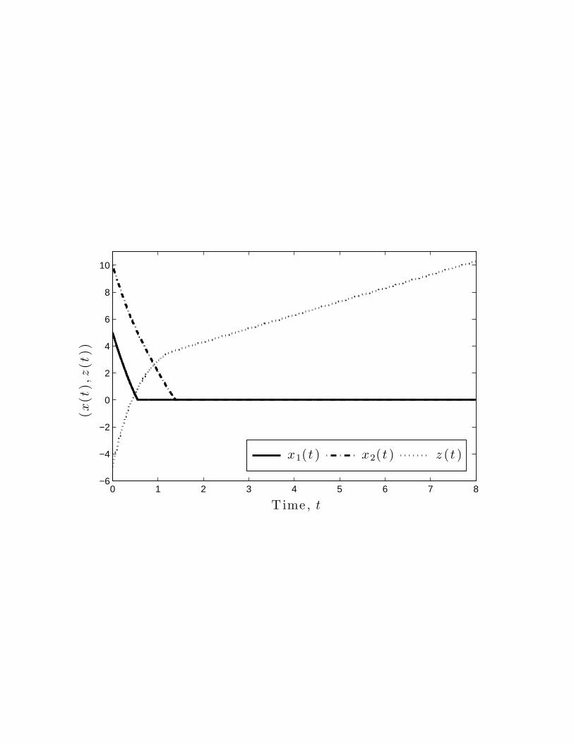
0 1 2 3 4 5 6 7 8−6

−4

−2

0

2

4

6

8

10

Time, t

(x(t

),z(t

))

x1(t ) x2(t ) z (t )

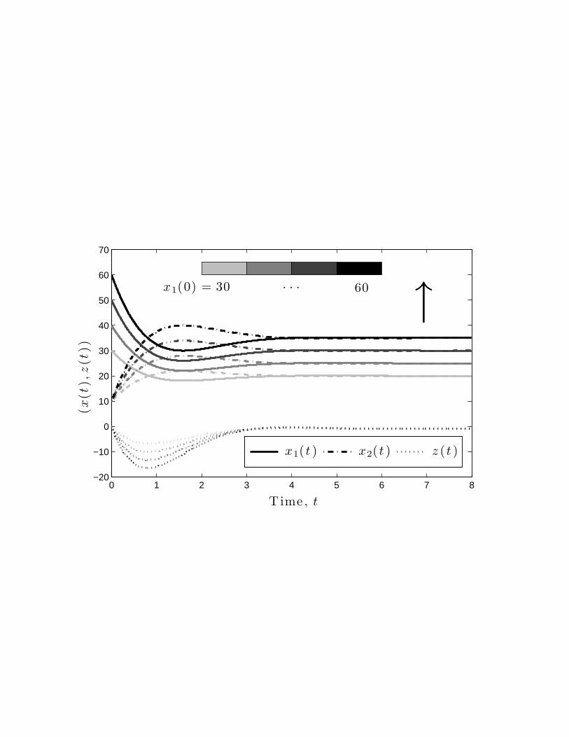
0 1 2 3 4 5 6 7 8−20

−10

0

10

20

30

40

50

60

70

→

Time, t

(x(t

),z(t

))

x1(0) = 30 . . . 60

x1(t ) x2(t ) z (t )

1 Robust distributed linear programming - arXiv · 1 Robust distributed linear programming Dean...

Documents

Transcript of 1 Robust distributed linear programming - arXiv · 1 Robust distributed linear programming Dean...