1

Robotic Cutting: Mechanics and Knife ControlXiaoqian Mu, Yuechuan Xue, and Yan-Bin Jia

Abstract—Skills of cutting natural foods are importantfor robots looking to play a bigger role on kitchen assis-tance. The basic objective of cutting is to achieve materialfracture via smooth movements of a kitchen knife, whichin the process performs work to overcome the materialtoughness, acts against the blade-material friction, andgenerates shape deformation. During a cutting action, theknife also experiences varying contacts with the materialand cutting board. This paper investigates how a roboticarm with force sensing drives the knife to cut through anobject in a sequence of three moves: pressing, touching, andslicing. Based on fracture mechanics, position, force, andimpedance controls are applied either separately or jointlyin the move sequence so the knife follows a prescribedcutting trajectory to split the object. Stabilities of thesecontrols are established. Experiments over several typesof fruits and vegetables have exhibited natural cuttingmovements like would be performed by a human hand.

Index Terms—Modeling of cutting, fracture mechanics,knife pressing, slicing, robot control.

I. INTRODUCTION

AUTOMATION of kitchen skills is an important steptowards the advent of multipurpose home robots,

which have long been a public fascination. Until todayrobotic kitchen assistance has been limited to washingand sorting dishes [1], carrying food trays [2], cookingpancakes and noodles [3], making burgers [4], etc.Robotic cooking has been carried out on prepared rawmaterials in very structured settings [5]. In food factorysettings, robots are typically capable of only one task,whether cutting meat, deboning, or butchering chicken.In our life, not so coincidentally, specialized tools aresold at stores or online also for single operations suchas slicing lettuce, peeling potatoes, chopping fruits andvegetables, and so on. To play a much bigger role in thekitchen, robots need to be versatile and general purpose— even on just one class of tasks.

*Support for this research was provided by the US National ScienceFoundation under Grant IIS-1651792. Any opinions, findings, andconclusions or recommendations expressed in this material are thoseof the authors and do not necessarily reflect the views of the NationalScience Foundation.

*We would like to thank labmate Prajjwal Jamdagni for discussionand for his help with fracture toughness measurements.

The authors are with the Department of Computer Science,Iowa State University, Ames, IA 50011, USA (e-mail: muxiao,yuechuan, jia@iastate.edu).

Food cutting, as an integral part of automatic mealpreparation, stands out as one of the ultimate tests onhuman-level dexterity for robots. Today, basic cuttingskills such as chop, slice, and dice are still out of theirreach. Manipulation of soft or irregularly-shaped fooditems aside, one main technical challenge for roboticcutting is how to plan and control a knife’s movementthrough a material while reacting to encountered forcesof different natures (fracture, friction, viscosity, andcontact) by the material and cutting board. Such controlneeds to utilize some knowledge about these forces aswell as shape deformations, which can be modeled basedon elasticity theories [6], [7] and fracture mechanics [8].

Although the goal of cutting is steady progress leadingup to a complete separation of the material, changingcontacts and path constraints divide the action intoperiods which bear specific control objectives. In oneperiod, for example, the knife needs to progress onmaterial fracture. In another period, the knife needs tocome to a stop as soon as its edge touches the cuttingboard.

This paper investigates how a robotic arm movesa kitchen knife to cut through objects smoothly. Theconsidered objects include vegetables such as potatoesand fruits such as apples that will undergo negligibledeformations during the cutting process. The work to bepresented bears a number of characteristics below.

1) It investigates an under-researched form of manip-ulation which alters the structure of the manipu-lated object in the process.

2) It studies a kitchen knife skill via a decompositioninto three phases (illustrated in Fig. 1): pressing,in which the knife moves downward along a pre-scribed trajectory until its edges makes contactwith the cutting board; touching, in which theknife softens its impact with the cutting board;and slicing, in which the knife separates the objectcompletely with its edge sliding on the boardacross the object’s bottom.

3) Each of the three phases above, with its own ob-jective and contact constraints, is carried out undera separate control strategy, whether on position,position/impedance, or position/force.

4) These control strategies, with stability analyses,make use of the fracture and frictional forces

Fig. 1. Three phases of cutting: pressing, touching, and slicing. The knife poses, drawn in purple, green, and blue, respectively, mark thebeginnings of pressing and touching, and the end of slicing. Also drawn are the visible contours of some intermediate poses. The red dots onthe cutting board mark several intermediate positions of the contact point between the knife’s edge and the board as the object is sliced through.

modeled based on fracture mechanics.5) Cutting experiments are performed on natural

fruits and vegetables (rather than artificial objectsas often studied in fracture mechanics).

The rest of the paper is organized as follows. Sec-tion II reviews works in related areas including fracturemechanics, cutting of soft tissues, and robot control. Sec-tion III characterizes the technical problem and presentsits underlying mechanics. In Section IV, cutting is di-vided into the aforementioned three phases, for each ofwhich a separate control strategy is devised to adjustto the changing contact situation. Section V describesthe results from cutting four types of fruits/vegetableswith a WAM Arm utilizing its two degrees of freedom(DOFs) in a vertical plane. Section VI extends thecutting strategy to a robotic arm with more DOFs inthe plane. Summary, discussion, and future work followin Section VII.

This paper has extended an earlier conference ver-sion [9] in several aspects. The knife orientation is nowcontrolled directly in the pressing phase, rather than ex-erted as a constraint, to allow more flexibility of cuttingand also simplify control. Impedance control is added tolessen the impact between the knife and cutting board.Stabilities are established for all the control strategies.The paper also extends the cutting scheme to a roboticarm with more than two DOFs in the cutting plane, andincludes extensive experiments for validation purpose.

II. RELATED WORK

Fracture mechanics [10] builds on a balance betweenthe work done by cutting and the total amount spentfor crack propagation, transformed into other energyforms (strain, kinetic, chemical, etc.), and dissipated byfriction. Methods for measuring the cutting force and

fracture toughness were studied for ductile materials [11]and live tissues [12], [13]. A “slice-push ratio” wasintroduced in [14] to quantify the works done alongtwo orthogonal directions, and then to formulate thedramatic decrease in the fracture force when the knifewas simultaneously pressing and slicing the material. Adifferent explanation [15] for such decrease stated thatpushing caused global deformation while slicing yieldedlocal deformation (and thus required less effort to createfracture). The fracture force and torque could be obtainedvia an integration along the edge of the blade [16]. Inour paper, this approach has been extended to accountfor blade-material friction in modeling.

Stress and fracture force analyses, supported by sim-ulation and experiment, were performed for roboticcutting of biological materials, accounting for factorssuch as blade sharpness and slicing angle [17]–[19]. Insurgical training, realistic haptic display of soft tissuecutting is quite important. Haptic models were developedfor animal tissue cutting with a scissor [20], soft tissuedeformation prior to fracture [21], as well as needleinsertion into soft tissues [22]. Most of these models,however, tended to be empirical. We refer to [23] for asurvey on mechanics and modeling of cutting biologicalmaterials.

The knife carries out cutting along some trajectorythrough contacts between its blade with the material andthe cutting board. While position control [24, pp. 190-199] realizes trajectory following, force control [25]robustly deals with modeling and execution errors incontact tasks. Since contacts experienced by the knifevary during a complete cutting action, it is natural toemploy multiple control policies. Hybrid force/positioncontrol [26], for instance, is a natural choice when theknife is slicing through an object while maintaining

2

Cutting Board

Object

Knife

Robotic Arm

b

ox

y py′′

a

θ1

x′

y′

l1

x′′

θ2

l2

Fig. 2. 2-D robotic arm cutting an object.

contact with the cutting board. Impedance control [27],which adjusts contact force from a motion deviationlike an intended mass-spring-damper, can be employedduring fast cutting to reduce the impact between theknife and cutting board. For the entire action of cut-ting to look natural, smooth transitions among thesepolicies would be desirable. Switching between positionand force controls was shown to regulate the contactforce during an impact and realize a smooth contacttransition [28].

To deal with contact constraints, controls of forceand position are more effectively conducted in theworkspace [29] using a reduced set of coordinates [30,pp. 501-510]. Keeping the knife’s orientation duringa period of cutting, sometimes desirable, can also becarried out as control of a constrained manipulator [24,pp. 202-203].

Robotic cutting has been investigated in a number ofways: adaptive control based on position and velocityhistory to learn the applied force [31], adaptive forcetracking via impedance control [32], visual servoing cou-pled with force control [33], and impedance control forcooperation of a cutting robot and a pulling robot [34].Adaptive impedance control was carried out to minimizeforce error in cutting a nonhomogeneous workpiece [32],utilizing a bound for the gain yielded from stabilityanalysis. A 2-DOF robot [35] demonstrated how todebone a bird by following a cutting path determinedfrom x-ray imaging based on force feedback, with thehelp of a passive mechanism for fixation.

Data driven robotic cutting has also been investigated.In [36], a generative model for representing objects’properties was created from collected haptic information,and predefined actions were chosen based on the model.Learning algorithms were proposed in [37] to estimatethe optimal input force for control during cutting.

III. MECHANICS OF CUTTING

A. Notation

In this paper, a vector is represented by a lowercaseletter in bold, e.g, a = (ax, ay)T , with its x- and y-coordinates denoted by the same (non-bold) letter withsubscripts x and y, respectively. A unit vector has a hat,e.g., a = a/‖a‖. The cross product a×b of two vectorsa and b is treated as a scalar. The subscripts d and e

refer to the desired value and error, respectively. Forexample, ayd and aye are the desired value and errorfor ay . A matrix is denoted by an upper case letter,e.g., A, and its pseudo-inverse has the superscript +,e.g., A+. An n× n identity matrix is denoted by In. Asuperscript in the form of a parenthesized number refersto the expression of the corresponding variable as givenin the equation referenced by that number, e.g., τ (32)

a

refers the expression of τ a in (32). Table I summarizesthe notation used in this paper.

B. Assumptions

As shown in Fig. 2, cutting of an object takes placein the vertical x-y plane, referred to as the world frame,located at some point o on the cutting board. Theblade of a knife is often quite thin. To have a cleanpresentation, we make the following assumption aboutthe knife used for cutting:(A1) The knife’s blade has negligible thickness.The knife is considered very sharp, which makes the nextassumption reasonable:(A2) Contact friction between the knife’s edge and

cutting board is negligible.Under assumption A2, when the knife’s edge touchesthe board, it receives an vertically upward contact force.This will facilitate control of slicing to be presented inSection IV-C.

Our next assumption is about the object:

3

TABLE INOMENCLATURE.

˙ Differentiation with respect to time.′ Referring to the knife frame.′′ Referring to the arm frame.o Origin of the world frame.p Knifes tip point (origin of the knife frame).a Arms open end (origin of the arm frame).c Knife-board contact (lowest point on knife).ψ Knife frame rotation from the world frame.ψ′′ Knife frame rotation (constant) from the

arm frame.R Knife’ rotation matrix.ω Knife’s angular velocity.θ1 First joint angle.θ2 Second joint angle.β Knife’s edge curve.γ Knife’s spine curve.κ Object’s fracture toughness.σ Object’s contour curve.Φ Fracture region.Ω Contact region.cm Knife’s center of mass.m Knife’s mass.g Gravitational acceleration.µ Coefficient of knife-object friction.P Knife-object pressure distribution.fC Fracture force.fF Frictional force.

fS Force reading by a F/T sensor.τC Torque on a due to fracture.τF Torque on a due to friction.ρa Wrench exerted at a.τ Joint torque vector.τ (n) Expression of τ given in equation (n).Ja Jacobian at a.Jc Jacobian at c.ιc Jacobian for coordinate transformation to cx.M Robotic arm’s mass matrix.C Matrix including the Coriolis and centrifugal

effects on the arm.In n× n identity matrix.τg Gravity term of the arm.τa Combination of Coriolis, centrifugal, gravitational,

and external forces at a.τ c Combination of Coriolis, centrifugal, gravitational,

and external forces at c.Kp|a,Ki|a,Kv|a Proportional, integral and derivative gain matrices

for position control during pressing, where a isthe point of interest.

kr, dr, br Desired stiffness, damping and mass for impedancecontrol during touching.

kfi Integral gain for contact force control.kp|c, ki|c, kv|c Proportional, integral and derivative gains for

position control during slicing, where c is thepoint of interest.

(A3) The object remains stable during cutting withnegligible dynamic effects.

The object is stabilized on its own (e.g, lying on a flatbase) or by some fixture. Dynamic effects are negligiblebecause cutting proceeds at a relatively slow speed.

Some foods such as potatoes and yams barely deformduring cutting. In this paper, we will relieve ourselvesfrom deformable modeling with the last assumption:

(A4) The material being cut has negligible deformation.

C. Task Geometry

The knife in Fig. 2 is rigidly attached to the open enda of a 2-DOF robotic arm, whose base is located at band whose two links of lengths l1 and l2 move in the x-yplane. The corresponding two joint angles are denotedby θ1 and θ2. At a is attached a frame x′′-y′′ referredto as the arm frame. Writing

θ = (θ1, θ2)T ,

l1 =

(cos θ1

sin θ1

), (1)

l2 =

(cos(θ1 + θ2)

sin(θ1 + θ2)

), (2)

p

vp

ω

r1

q1

x′

ds

r3r4

r2u1

u2

Spineγ(q)

Ψβ(u)Edge

y′

q2

σ(r)

o

y

x

Φ

Fig. 3. Geometry of cutting.

we obtain the arm frame’s position

a =

(axay

)= b+ l1l1 + l2l2, (3)

and orientationφ = θ1 + θ2. (4)

Attached to the knife point p is a local frame x′-y′

(see Fig. 2), called the knife frame. This frame, rigidlyconnected to the arm frame x′′-y′′, rotates from the latterthrough a constant angle ψ′′, and thus, from the worldframe through an angle

ψ = θ1 + θ2 + ψ′′. (5)

The shapes of kitchen knives differ by culture. Somehave straight edges and spines, and some have curvedones. The kitchen knife considered here has both curved

4

edge and spine, in part because knives of this type arequite common, and in part because straight edge andspine can be considered as special cases of curved ones.As depicted in Fig. 3, the knife’s edge and spine aredescribed in its own x′-y′ frame by two curves β′(u) =(β′x, β

′y)T and γ′(q) = (γ′x, γ

′y)T , respectively, such that

β′(0) and γ′(0) coincide with the frame’s origin at theknife point p. In the world frame x-y, they are thusdescribed by the following two curves:

β(u) =

(βxβy

)= p+R(ψ)β′(u), (6)

γ(q) =

(γxγy

)= p+R(ψ)γ′(q),

whereR(ψ) =

(cosψ − sinψsinψ cosψ

)is the rotation matrix for the knife.

As cutting proceeds, the edge intersects the object ata section of β(u) over some interval [u1, u2], u1 ≤ u2.That u1 = u2 holds at the start (time t = 0) andend of cutting. The section is denoted β[u1, u2] forconvenience. A section γ[q1, q2] of the spine γ(q) over[q1, q2], for some q1 and q2, may also be inside theobject. Both curve sections are illustrated in Fig. 3.

Since the object does not deform under Assump-tion A4, we let the curve σ(r) describe its non-varyingcontour of the cross section intersected by the x-y plane.The knife’s edge intersects the curve at σ(r1) and σ(r2)from left to right. Clearly,

β(u1) = σ(r1),β(u2) = σ(r2).

The segments β[u1, u2] and σ[r2, r1] enclose the frac-ture region Φ (see Fig. 3). When a section of the spineγ[q1, q2] is inside the cross section, it is bounded byσ(r4) and σ(r3) such that

γ(q1) = σ(r4),γ(q2) = σ(r3).

The four segments β[u1, u2], σ[r2, r3], γ[q1, q2], andσ[r4, r1] bound the contact region Ω. Clearly, Ω ⊆ Φ.

D. Forces During Cutting

During cutting, let vp be the velocity of the knifepoint p, and ω the knife’s angular velocity. The edgesegment β[u1, u2] experiences a force fC due to mate-rial fracture. In other words, the work done by −fC isyielding new fracture.1 Consider an infinitesimal element

1On a deformable object, the knife would also exert a force −fUwhich causes an increase (or decrease) in the object’s strain energy.

dsdη

ν

t

−dfC

n

Fig. 4. Area of fracture yielded by an element of length ds on theknife’s edge.

of length ds on the knife’s edge starting at u ∈ [u1, u2].See Fig. 4. The element may or may not be generat-ing fracture under the knife’s rotation. We need onlyconsider the former case here. The element exerts theforce −dfC in the direction of its velocity

ν = vp + ωR(ψ)

(−β′yβ′x

),

and for a movement of distance dη, generates an areaof fracture that is a parallelogram (shown in Fig. 4). Itsfour sides are parallel to either the edge tangent

t =

(dβxdu

,dβydu

)/∥∥∥∥(dβxdu , dβydu)∥∥∥∥

or the velocity ν. The material’s fracture toughness κ isdefined to be the energy required to propagate a crackby unit area [10, p. 16]. We have

(−dfC · ν)dη = −κ(ν · n)dηds,

where n is the unit inward normal at β(u), ν = ν/‖ν‖,and

dfC = κ(ν · n)ν ds

= κ

(ν ·(−dβydu

,dβxdu

)T)ν du.

Integration over the segment S = β[u1, u2] yields thetotal fracture force:

fC =

∫S

dfC . (7)

Since the knife is rigidly attached to the robotic arm’sopen end a, the fracture force yields a torque at thepoint:

τC =

∫S

(β(u)− a)× dfC . (8)

Coulomb friction exists in the contact region Ω onboth sides of the blade. Denote by fF the frictional forceexerted on the knife. Let P be the pressure distributionand µ the coefficient of friction. Let the unit vectorv(x, y) donate the direction of the velocity of an area

5

element at (x, y)T ∈ Ω. The force and torque at the openend a due to friction are given below:

fF = −2µP

∫ ∫Ω

v dxdy, (9)

τF = −2µP

∫ ∫Ω

((x

y

)− a

)× v dxdy. (10)

The wrenches (fC , τC) and (fF , τF ) will be used forknife control during touching and slicing in SectionsIV-B and IV-C later. They can be evaluated given theknife’s pose (p, ψ) and velocities (vp, ω). If the knife istranslating, they have simple forms that are derived inAppendix A. In the general case, the velocities of thepoints on the knife edge and inside the contact area Ωvary, which implies that the fracture and frictional forcesand torques can only be calculated numerically.

Besides causing fracture and overcoming friction, thearm needs to balance the knife’s gravitational forceand its resulting torque. The wrench (force and torque)exerted at the arm’s open end a due to cutting, friction,and knife gravity is

ρa =

(fC + fF −mgy

τC + τF −mg(cm − a)× y

),

where m is the knife’s mass, cm the location of itscenter of mass, g > 0 the gravitational acceleration, andy = (0, 1)T . The wrench is measured by a force/torque(F/T) sensor mounted at a (whose location is effectivelyextended by the sensor).

IV. DYNAMICS AND CONTROL OF CUTTING

Cutting of an object proceeds in three phases that werepreviously illustrated in Fig.1. The first phase is pressing,during which the arm translates the knife downward untilits edge contacts with the cutting board. The second(transitional) phase is touching during which the armreduces the magnitude of knife’s vertical velocity tosoften the robot-knife contact. The third phase is slicingduring which the arm translates and rotates the knife tomove its contact point with the cutting board across theobject’s bottom segment plpr in the cutting plane. Bynow the object has been split into two parts.

A. Pressing

The relative position and orientation of the arm frameto the world frame is described by the vector x =(aT , φ)T , with a and φ given in (3) and (4), respectively.Immediately,

x = Jaθ, (11)

where Ja is the 3× 2 Jacobian at a:

Ja =∂

∂θ

(b+ l1l1 + l2l2

φ

).

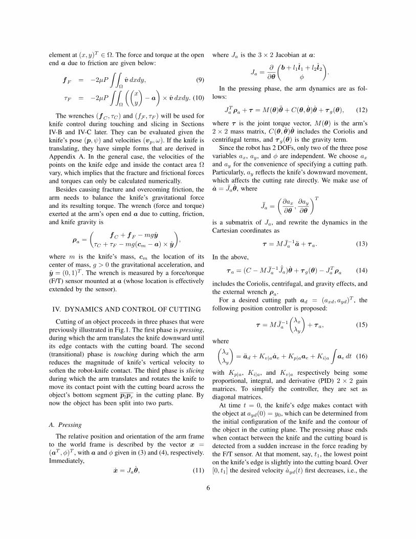
In the pressing phase, the arm dynamics are as fol-lows:

JTa ρa + τ = M(θ)θ + C(θ, θ)θ + τ g(θ), (12)

where τ is the joint torque vector, M(θ) is the arm’s2 × 2 mass matrix, C(θ, θ)θ includes the Coriolis andcentrifugal terms, and τ g(θ) is the gravity term.

Since the robot has 2 DOFs, only two of the three posevariables ax, ay , and φ are independent. We choose axand ay for the convenience of specifying a cutting path.Particularly, ay reflects the knife’s downward movement,which affects the cutting rate directly. We make use ofa = Jaθ, where

Ja =

(∂ax∂θ

,∂ay∂θ

)Tis a submatrix of Ja, and rewrite the dynamics in theCartesian coordinates as

τ = MJ−1a a+ τ a. (13)

In the above,

τ a = (C −MJ−1a

˙Ja)θ + τ g(θ)− JTa ρa (14)

includes the Coriolis, centrifugal, and gravity effects, andthe external wrench ρa.

For a desired cutting path ad = (axd, ayd)T , the

following position controller is proposed:

τ = MJ−1a

(λxλy

)+ τ a, (15)

where(λxλy

)= ad +Kv|aae +Kp|aae +Ki|a

∫ae dt (16)

with Kp|a, Ki|a, and Kv|a respectively being someproportional, integral, and derivative (PID) 2 × 2 gainmatrices. To simplify the controller, they are set asdiagonal matrices.

At time t = 0, the knife’s edge makes contact withthe object at ayd(0) = y0, which can be determined fromthe initial configuration of the knife and the contour ofthe object in the cutting plane. The pressing phase endswhen contact between the knife and the cutting board isdetected from a sudden increase in the force reading bythe F/T sensor. At that moment, say, t1, the lowest pointon the knife’s edge is slightly into the cutting board. Over[0, t1] the desired velocity ayd(t) first decreases, i.e., the

6

y

x prpl

oc

fy

Fig. 5. Knife touching the cutting board.

speed |ayd(t)| increases, and then stays at a constantvalue.

During pressing, the desired path is often chosen to beone with constant end-effector orientation so the knifeis in translation, in order to simplify the calculation offracture and frictional forces.

B. Touching

The initial point of contact in the touching phase

c =

(cxcy

)= p+R(ψ)β′(u) (17)

needs to start to the left endpoint pl of the object’sbottom segment (see Fig. 5). This can be done by settingthe desired trajectory ad properly.

The upward contact force is represented by a scalar fy .This force is a component of the total force fS receivedat the open end a, which is part of ρa from the readingby the F/T sensor mounted at a, that is

fS = fC + fF + (fy −mg)y. (18)

Here, the fracture force fC and the friction force fFare obtained from modeling described in Section III.Therefore, we can estimate fy using the above equationto control it later.

Under the knife-board contact, the dynamics haschanged from (12) to

τ = M θ + Cθ + τ g − JTa ρa − JTc(

0

fy

), (19)

where, from (17),

Jc =∂c

∂θ=∂p

∂θ+∂R(ψ)

∂θβ′(u) (20)

(u treated as a constant) is the Jacobian of c. Dif-ferentiating a = Jaθ and substituting the obtainedθ = J−1

a (a− ˙Jaθ) into (19), we transform it to

τ = MJ−1a a+ τ a − JTc

(0

fy

). (21)

A large contact force could halt the arm or even causesome damage to it, so the robot has a need to decelerateas soon as contact with the cutting board is detected.

x

yx′

oprpl

y′

c,β(u)

x′′y′′

θ2

Fig. 6. Slicing along the cutting board.

Impedance control in the following form can achievethe purpose:

τ = MJ−1a

(λxλ′y

)+ τ a − JTc

(0

fy

), (22)

where the servo λx in the x-direction is given in (16)with zero desired velocity and acceleration, while theservo in the y-direction is

λ′y = ayd +kraye + draye + fy

br,

where kr, dr, and br are some stiffness, damping,and inertia values for a desired impedance behavior,respectively.

The reason for using impedance control rather thanforce control is that the former handles velocity to makeits behavior similar to a damper. Force control, on theother hand, does not quite perform as adaptively to theimpact velocity.

Impedance control ends when the contact force varieslittle after a significant decrease. Since this type ofcontrol is known not for precise force regulation, furtheradjustment of the contact force will follow.

C. Slicing

Slicing starts right after touching. During this phase,the knife moves on the cutting board to split the object.To ensure separation, the knife-board contact force ismaintained at some desired level throughout the phase.As illustrated in Fig. 6, the arm frame x′′-y′′ rotates inorder to keep the knife-board contact, which as a resultmoves on both the knife’s edge (located by β(u)) andthe board (located by c). The knife undergoes a changingrotation of the angle ψ given in (5) from the world frame.The knife point is at

p = a+R(ψ)p′′,

where p′′ is its (fixed) position in the arm frame. Itfollows from (6) that the moving edge curve β depends

7

Robot

Kinematics

Model

Controller

F/T Sensor

-

+

Desired Inputs

+

+

+

+

+

+

+

+

++

+ -

- +

+

+

+

-

- -

-

(a) (b)Fig. 7. Control schemes for (a) the entire action of cutting and (b) hybrid control used in the slicing phase.

on ψ, and therefore on the joint angles θ. The contactpoint β(u) on the curve is at c = (cx, 0)T . Thus,

βx = cx, (23)βy = 0. (24)

The contact point c is the lowest point on β, satisfying

∂βy∂u

= 0. (25)

Equations (23)–(25) define θ1, θ2, and u as functionsof cx

2. Given cx, we can solve for θ1, θ2, and uusing Newton’s method or the homotopy continuationmethod [38]. This prompts us to replace θ with cx,since the rest of cutting reduces to moving the pointc from pl to pr along the x-axis. The Jacobian for theabove coordinate transformation is

ιc =dθ

dcx, (26)

so thatθ = ιccx. (27)

The derivative ιc, along with du/dcx, can be solved fromthe three linear equations generated from differentiat-ing (23)–(25) with respect to cx. For details, we refer toAppendix B.

The motion of the knife during slicing is restricted byits contact with the cutting board. The dynamics given

2Equations (24) and (25) alone define a curve θ(u) =(θ1(u), θ2(u))T in the joint space, which ensures the knife to stay incontact with the table as it moves.

in (21), after the substitution θ = ιccx + ιccx fromdifferentiating (27), are transformed into

τ = Mιccx + τ c − JTc(

0

fy

), (28)

where

τ c = M ιccx + Cθ + τ g − JTa ρa. (29)

The knife-board contact force fy is estimated from mod-eling and the reading by the F/T sensor using (18). Thederivative ιc can be evaluated from differentiating (23)–(25), which is also detailed in Appendix B.

Let cxd(t) be some desired time trajectory of cx andcxe(t) = cxd − cx be the position error of the contactpoint c. The desired constant normal force exerted onthe table is −fd. The force error is fe = fd − fy . Wenow apply a third control law below:

τ =Mιc

(cxd + kv|ccxe + kp|ccxe + ki|c

∫cxe dt

)+ τ c − JTc

(0

fd + kfi

∫fe dt

), (30)

where kp|c, ki|c, and kv|c are the PID gains, respectively,and kfi is the integral gain for regulating the contactforce.

D. Control Architecture and Stabilities

Fig. 7 (a) shows the basic system diagram, in whichthe controller handles all the position and force inputsfrom specifications, the kinematics of the arm, F/Tsensor, and modeling. Part (b) of the figure details hybrid

8

position/force control in the slicing phase. Stabilities ofthe controllers (15), (22), and (30) applied in the threecutting phases are established in Appendix C.

V. EXPERIMENTS

Fig. 8. Experimental setup. Joints 2 and 4 of a WAM arm are mappedto the joints of the 2-link arm in Fig. 2 with θ1 = θW2 + 1.652433and θ2 = θW4 − 0.209506, where θW2 is the angle of joint 2 andθW4 is that of joint 4. The equivalent lengths of the two links arel1 = 0.551838 m and l2 = 0.352881 m.

TABLE IIPHYSICAL PARAMETERS FOR CUTTING: BLADE-MATERIAL

COEFFICIENT OF FRICTION µ, FRACTURE TOUGHNESS κ, ANDPRESSURE DISTRIBUTION P .

Objects µ κ (N/m) P (N/m2)

0.477 675 2927

0.7 270 2000

0.6 400 2700

0.7 370 2500

Shown in Fig. 8, the arm used for cutting was a4-DOF Whole Arm Manipulator (WAM) from BarrettTechnology, LLC. Its joints 1 and 3 were fixed sothe robot effectively had two DOFs. We derived the

arm’s dynamics equation (12) according to its specifi-cations [39].

Mounted on the end effector was a 6-axis DeltaIP65 F/T sensor from ATI Industrial Automation. Itsgeometry, mass, and inertial properties are available. AMicrosoft Kinect sensor was used in acquiring somedensely distributed points on the object’s surface. Thosepoints close enough to the cutting plane were fit over toconstruct the contour σ(r) of the cross section, where ris the x-coordinate in the world frame. The kitchen knifewas rigidly mounted on the F/T sensor using a metaladaptor, so its kinematics were in terms of the robot’sjoint angles. Before cutting, the robotic arm moved to afix position where the knife was not in contact with theobject.

A 4-DOF Servo Motor Arm was used to stabilizethe object during cutting. The small arm could alsorepeatedly push the uncut portion of the object forwardon the cutting board for a specified distance.

To model a kitchen knife, we placed it on a sheet ofpaper, and drew its contour. The knife’s edge β′(u) wasreconstructed in the knife frame x′-y′ as follows. Settingu to be the x′-coordinate, we fit a quadratic curve β′y tothe y′-coordinates of the measured points on the edge.Similarly, the knife’s spine was reconstructed throughfitting as a quadratic curve γ′(q) = (q, γ′y(q))T with qidentified with x′.

To measure the coefficient of friction between theblade and a material, we cut an object of this materialin half by hand and let one resulting piece rest withits newly cut face on the knife’s blade. Then we tiltedthe blade until the piece began to slide. The tangent ofslope angle for the blade at this moment was used as theestimate.

To measure the fracture toughness and pressure dis-tribution, the robot drove the knife to cut into an objectof the same type. During this process, the F/T sensorobtained a sequence of readings, each accounted forboth the fracture and frictional forces. Next, the armmoved the knife upward until it was above the pieceand then moved it downward into the crack for a secondtime. The new sequence of readings produced duringthis descent accounted for the frictional force only.Readings from the two sequences had a correspondenceby the height of the knife. Subtraction of the readingsin the second sequence from the corresponding onesin the first sequence recovered fracture force valuesduring the cutting action. The work done by the knifeduring cutting was thus estimated, so was the material’sfracture toughness via division by the measured fracturearea. The pressure distribution was estimated, during theknife’s second descent, from the frictional force readings

9

TABLE IIICONTROL GAINS FOR INDIVIDUAL PHASES OF CUTTING IN THE EXPERIMENTS.

Pressing Touching Slicing

Kp|a Ki|a Kv|a kp|a ki|a kv|a br kr dr kp|c ki|c kv|c kfi

500I2 800I2 35 I2 500 800 35 10 200 100 500 800 35 5

Fig. 9. Three phases of cutting an onion (t1 = 0.916 s, t2 = 0.98 s, and t3 = 2.69 s): pressing (a)–(f), touching (g)–(h), and slicing (i)–(k).(a) Snapshot of pressing (where the dashed edge is plotted to approximate the occluded portion of the knife’s edge). (b)–(c) Actual and desiredtrajectories of the arm’s open end a = (ax, ay)T and (axd, ayd)T . (d) Actual and desired knife orientations θ1 + θ2 and θ1d + θ2d. (e)-(f)Trajectories of the sensed force fS = (fSx, fSy)T , modeled fracture force fC = (fCx, fCy)T , and friction force fF = (fFx, fFy)T . (g)Snapshot of touching. (h) Sensed force in the y-direction during the phase. (i) Snapshot of slicing. (j) Actual and desired trajectories of theknife-board contact point on the cutting board as respectively located by the coordinates cx and cxd, and the point’s changing location s onthe knife’s edge. (k) Desired normal contact force fd and the y-components of the sensed, frictional, and fracture forces.

and the areas of the blade inside the object at the sametime instants.

Onions, potatoes, apples, and cucumbers were used

in the experiment. Table II lists the measured values ofthe physical parameters for these four types of objects.These parameter values could vary with freshness of the

10

food item and the thickness of its parts on both sides ofthe blade.

In a cutting trial, half of an object (precut by thehuman hand) was placed on a table with its flat facedown (see the potato in Fig. 8).

Values of the control gains for all the three phases ofcutting are listed in Table III. Applied to all four objecttypes, these gains were chosen to keep the robotic armstable and from generating excessive torque responses atits joints. Such an undesired situation could occur, forinstance, with impedance control during touching if avery large value for the gain dr is chosen, commandingtorques to exceed the limits for the arm.

A. Phase-by-Phase Control Validation

Cutting starts with the knife making an initial contactwith the object. The arm’s joint angles can be calculatedfrom a preselected knife orientation. The three phases ofpressing, touching, and slicing are carried out over thetime periods [0, t1), [t1, t2), and [t2, t3], respectively.

Pressing. Fig. 9 presents the data obtained fromcutting an onion. The pressing phase ended with an errorof 0.8 mm in the open end’s x-position, an error of1.3 mm in its y-position and a deviation of 0.002 radin its orientation (see the plots in (b)-(d)). The plotin (e) shows that the sensed force fS and the sumof the modeled fracture force fC and frictional forcefF has an average discrepancy around 8 N in the ydirection. Their discrepancy in the x direction as shownin (f), is around 2 N on the average. These discrepancieswere mainly due to two factors. One was the inaccuratecontour σ(r) of the cross section, which was obtainedby fitting over points acquired by the Kinect sensor. Theother factor was that the three parameters (µ, κ, and P )varied slightly from one object to another of the sametype.

Touching. This phase was detected from a suddenincrease in the y-component of the force reading astriggered by the knife’s contact with the cutting board.Fig. 9(g) shows a snapshot from this second phaseof the same cutting action. As plotted in Fig. 9(h),the knife-board contact force under impedance controlstopped the increase quickly and then started to decrease.Since the knife barely moved, the fracture and frictionalforces were negligible so the knife-board contact forceaccounted for the y-component of the sensor reading.The touching phase ended after this contact force hadbecome stabilized.

Slicing. A snapshot of the following slicing phaseof the action is shown in Fig. 9(i). The knife wastranslating and rotating, which resulted in a movement

by the contact point for a distance (i.e., change in s) thatwas neither zero nor equal to that (i.e., change in cx) ofits movement on the cutting board. This is illustrated byan increasing gap between the s and cx trajectories in(j). As shown in (k), the contact force component fy wasmaintained close to the desired value. This componentwas estimated by subtracting from the sensor readingthe modeled fracture and knife-material friction forces(which were close to 0). The end of slicing was detectedvisually after the knife-board contact point moved out ofthe object.

B. Complete and Repeated CuttingFig. 10(a)–(e) shows the experimental results from

cutting a potato. Included in (a) are four snapshotsrespectively at the start and during the three phases. Herewe let c = (cx, cy)T also denote the lowest point on theknife’s edge during the pressing and touching phases.In (b), the ordinate cy follows the desired trajectorycyd (which was obtained from ayd, since the knife wasrigidly connected to the robot) during pressing, and theabscissa cx follows the desired trajectory cxd throughoutthe three phases of cutting. Fig. 10(c), plotted over theperiod [t1, t3], shows that the contact force decreasedquickly under impedance control during touching, andthen converged to the desired value with small varia-tions under force control during slicing. In the pressingphase, as shown in (d), the modeled frictional force fF(between the blade and the material) and fracture forcefC add up close to the sensed force fS . The same plotalso shows that, during slicing, the y-component of themodeled fF + fC was very small, since every pointon the knife edge was moving close to the x-direction.Also shown in (d), the force reading at the start of cuttingwas not zero in x or y directions. This was due to aninaccurate contour reconstructed from points obtainedfrom the Kinect sensor so the knife had been pressingagainst the object already before cutting started. In (e),the orientation θ1 + θ2 of the arm frame (hence that ofthe knife) stays almost constant in the first two phases,and increases in the third phase since the knife had torotate to maintain its contact with the cutting board.

Convergence to the desired knife motions and forcemagnitudes were also observed in apple cutting of whichan instance is shown in Fig. 10(f)–(h).

The robotic arm could perform cutting actions in asequence. Fig. 11 includes some snapshots from cuttinga cucumber into pieces.

VI. CUTTING WITH HIGHER DEGREES OF FREEDOM

The three-phase cutting strategy presented in Sec-tion IV can be extended for a robotic arm with n > 2

11

Fig. 10. Results from cutting of a potato (a)–(e) and an apple (f)–(h). (a) Snapshots of cutting the potato (t1 = 0.908 s, t2 = 0.97 s, andt3 = 2.528 s). Trajectories of the (b) lowest point c on the knife, (c) contact force between the knife and cutting board in the y-direction, (d)force fS = (fSx, fSy)T exerted on the knife as obtained from sensor readings, modeled fracture force fC = (fCx, fCy)T , and modeledfrictional force fF = (fFx, fFy)T , and (e) sum of the two joint angles. (f) Snapshots of cutting the apple (t1 = 0.786 s, t2 = 0.85 s, andt3 = 2.554 s). Trajectories of (g) the lowest point c, and (h) the actual and desired contact forces fy and fd.

Fig. 11. Snapshots of cutting a cucumber into eight pieces.

revolute joints which have parallel horizontal axes (sotheir driven links can be viewed as moving in thesame vertical plane). The extra DOFs make it possiblefor the arm to maintain the knife’s orientation duringthe third phase of slicing. The unit link directions l1and l2 defined in (1) and (2) now assume the formsli = (cos(

∑ij=1 θj), sin(

∑ij=1 θj))

T , i = 1, . . . , n.The arm frame has the orientation φ =

∑nj=1 θi and

the Jacobian Ja = ∂x/∂θ is now a 3 × n matrix.Denote by J+

a the pseudo-inverse of Ja. Except for

some degenerate arm configurations, the rows of Ja arelinearly independent and J+

a = JTa (JaJTa )−1, so that

JaJ+a = I3. (31)

Redefine τ a introduced in (14) as

τ a = (C −MJ+a Ja)θ + τ g − JTa ρa (32)

and substitute

τ = MJ+a x+ τ (32)

a (33)

into the arm dynamics (12). In the resulting equation, weutilize (31) and the non-singularity of the mass matrix Mto obtain

θ = J+a (x− Jaθ),

which clearly satisfies the equation

x = Jaθ + Jaθ

obtained from differentiating the kinematics (11). Equa-tion (33) describes, in the Cartesian coordinates, correctarm dynamics because they are consistent with thekinematics.3

3Note that J+a can be replaced with any right inverse A of Ja to

yield arm dynamics consistent with (33).

12

Now we let xd = (aTd , φd)T be some desired trajec-

tory and xe = xd−x be the error. The controller in thepressing phase is derived from (33) by replacing x with λx

λyλφ

= xd +Kv|axe +Kp|axe +Ki|a

∫xe dt,

where Kv|a, Kp|a, and Ki|a are all 3×3 positive-definitediagonal matrices. This results in the following closedloop system:

MJ+a

(xe +Kv|axe +Kp|axe +Ki|a

∫xe dt

)= 0.

Multiplication of the above with JaM−1 and utilizationof (31) yield the error dynamics:

xe +Kv|axe +Kp|axe +Ki|a

∫xe dt = 0,

for which stability analysis is similar to that given inAppendix C-A for the controller (15) for a 2-DOF arm.

Starting in the touching phase, the knife is in contactwith the cutting board. In this phase, the arm dynamicshave an extra term than in (33) due to the contact forcefy exerted by the cutting board:

τ = MJ+a x+ τ (32)

a − JTc(

0

fy

), (34)

where Jc, introduced in (20), is now a 2 × n matrix.Impedance control takes a form similar to (22):

τ = MJ+a

λxλ′yλφ

+ τ (32)a − JTc

(0

fy

). (35)

Stability analysis will be presented in Appendix D.With more than two degrees of freedom, the arm can

perform slicing without rotating the knife if needed.Lowest on the knife’s edge curve β(u), the contactpoint c satisfies (25), which induces the parameter valueu = ζ(θ) for some function ζ. That this point lies onthe cutting board introduces a constraint

βy(ζ(θ)) = 0.

Under the new constraint, the independent variables arechosen to be cx and φ, where cx = βx(ζ(θ)). Lettingy = (cx, φ)T , we have

y =

(cxφ

)= Jcθ, (36)

where

Jc =∂y

∂θ.

Via a substitution of the expression of θ obtained fromdifferentiating (36), the system dynamics (19) for touch-ing are transformed into

τ = MJ+c y + τ c − JTc

(0

fy

), (37)

where J+c is the pseudoinverse of Jc such that JcJ+

c =I2, and τ c is redefined from (29) below:

τ c = (C −MJ+c

˙Jc)θ + τ g − JTa ρa. (38)

To completely separate the object, during the slicingphase the knife maintains a certain level of force on theboard to keep in direct contact. Let cxd(t) and φd(t)be the desired trajectories of cx and φ, respectively. Wewrite yd = (cxd, φd)

T . The following hybrid controller

τ = MJ+a

(λxλψ

)+ τ (38)

c − JTc(

0

fd + kfi

∫fe dt

),

(39)where(

λxλψ

)= yd +Kv|cye +Kp|cye +Ki|c

∫ye dt,

is proposed to realize the rate cxd(t) of separation whilemaintaining the knife’s constant orientation.

VII. DISCUSSION AND FUTURE WORK

This paper is about how to enable a robotic arm toperform a natural and smooth cutting action. We havesequenced the entire action into three phases (pressing,touching, and slicing), drawing inspirations from kitchenknife maneuvers by the human hand. Given the action’scomplexity and the heavy presence of contacts (with theobject and cutting board) engaged by the knife, a singlepolicy such as position control is clearly inadequate forcarrying out the task robustly. Instead, different con-trol policies are employed sequentially to accommodatetheir own subgoals and specific contact constraints. Asdemonstrated in our experiments, these controls havesmooth transitions to cut open a fruit/vegetable in about2.5 s (see the submitted video).

Modeling based on fracture mechanics allows us toseparate, from the F/T sensor reading, forces of differentsources such as fracture, knife-material contact, andknife-board contact. In this work, we are able to estimatethe knife-board contact force using modeled fracture andfractional forces, and consequently carry out impedanceand hybrid controls during the touching and slicingphases.

An immediate extension will be to an object undergo-ing small deformations when it is being cut. Fracture andfriction forces needed for cutting control, along with the

13

areas of fracture and contact and the object’s shape andstrain energy, can be modeled using the finite elementmethod (FEM) based on fracture mechanics.4 For cuttingtrajectory planning and real-time plan adjustment, itis quite important to efficiently generate reliable forceand shape predictions along a hypothesized trajectory.Meanwhile, a vision system may be employed to helpreduce errors in shape tracking. We expect to compensatemodeling inaccuracies with force sensing and improvedknife control strategies. In the longer term, we would liketo investigate cutting of objects with large deformationsand viscosities. Modeling of strain energies and viscousforces can be quite important.

Another direction of extension is to have the kitchenknife held by a robotic hand driven by an arm ratherthan rigidly attached to the arm. The system will becomemore autonomous since the hand can pick up and regraspthe knife. There will be more dexterity because controlof the knife is directly done by the hand. Cutting controlwill have to take into account issues such as higherdegrees of freedom, compliance of contact between theknife’s handle and the hand, and (even possibly) fingergaits for adjusting a grasp on the knife. Involvementof a second robotic arm or hand to stabilize the objectbeing cut will bring up the challenging issue of two-handcoordination, which expects the development of somecontrol strategy to allow force interactions between thetwo hands.

At a higher level, we will look at how to plantrajectories to implement different knife skills includingchop, slice, and dice. Realization of a composite skillsuch as dice, for instance, needs to tackle the subproblemof cutting in a non-vertical plane (which can be a directextension to the current work).

APPENDIX ACOMPUTATION OF FRACTURE AND FRICTIONAL

FORCES FOR A TRANSLATING KNIFE

When the knife keeps a constant orientation, all thepoints on its blade are moving at the same velocity v.Denote v = v/‖v‖ = (vx, vy)T . Calculation of fractureand frictional forces and torques can be simplified. Theintegral (7) now has a closed form:

fC =

∫ u2

u1

κv ·(−dβydu

,dβxdu

)Tv du

= κ

(v ·(−βyβx

)∣∣∣∣u2

u1

)v.

(40)

4Some preliminary work [40] was recently carried out by othermembers of the authors’ lab.

The torque is determined using (8):

τC =

∫ u2

u1

(β(u)− a

)×(κv ·

(−dβydu

,dβxdu

)Tv

)du

= κv ·∫ u2

u1

((β(u)− a)× v

)(−dβydu

,dβxdu

)Tdu

= κv ·(−(−βyβx

)∣∣∣∣u2

u1

(a× v) +1

2

(β2y vx

β2xvy

)∣∣∣∣u2

u1

−∫ u2

u1

(βxβ

′y vy

β′xβy vx

)du

). (41)

Under Green’s theorem, the area A of the knife-material contact can be calculated along its boundary∂Ω as follows:

A =

∫ ∫Ω

dxdy =

∮∂Ω

x dy

=

∫ u2

u1

βx dβy +

∫ r3

r2

σx dσy +

∫ q1

q2

γx dγy

+

∫ r1

r4

σx dσy.

(42)

The frictional force (9) and its generated torque (10) are

fF =− 2µPAv, (43)

τF =− 2µP

∫ ∫Ω

((x

y

)− a

)× v dxdy

= 2µPAa× v − 2µP

∫ ∫Ω

(x

y

)× v dxdy

= 2µPAa× v − 2µP

∫ ∫Ω

(xvy − yvx) dxdy

= 2µPAa× v − 2µP

∫∂Ω

(x2

2vy − xyvx

)dy.

(44)The integrals (40)–(44) have closed forms when the

curves β, γ, and δ for the knife’s edge and spine andthe object’s cross section are parameterized using poly-nomials. Such parameterizations are easy to generate, asconducted in our experiments in Section V.

APPENDIX BJACOBIAN EVALUATION

In this appendix, we evaluate the Jacobian ιc definedin (26) and its derivative ιc related to the knife-boardcontact c. They are used for control in the slicing phase.Writing ξ = (θ1, θ2, u)T , so β is a function of ξ, wedifferentiate (23)–(25) with respect to cx:

dβ

dcxd

dcx

(∂βy∂u

) = B

dξ

dcx=

100

, (45)

14

where the 3× 3 matrix B is

B =

∂β

∂ξ∂

∂ξ

(∂βy∂u

) . (46)

Solving the linear system (45), we obtain dξ/dcx andthus ιc since

dξ

dcx=

ιcdu

dcx

. (47)

Next, we evaluate the derivative

ιc =

(d2θ1

dc2x,d2θ2

dc2x

)Tcx. (48)

The time derivative of cx is from differentiating (23):

cx =∂cx∂ξξ,

Among the components of ξ, θ1 and θ2 are read fromthe controller of the robotic arm, and u is obtained fromdifferentiating (25):

u = −(∂2βy∂θ1∂u

θ1 +∂2βy∂θ2∂u

θ2

)/∂2βy∂u2

.

What remain to be evaluated in (48) are the two partialderivatives d2θ1/dc

2x and d2θ2/dc

2x. It suffices to obtain

d2ξ/dc2x. Differentiation of (45) with respect to cx yields

dB

dcx

dξ

dcx+B

d2ξ

dc2x= 0,

from which we have

d2ξ

dc2x= −B−1 dB

dcx

dξ

dcx.

Of the three factors in the right hand side of the aboveequation, the matrix B = (bij) by (46) and derivativedξ/dcx by (47) are both available. The final step is toevaluate the 3× 3 matrix dB/dcx = (dbij/dcx), where

dbijdcx

=dbijdξ

dξ

dcx.

The partial derivatives dbij/dξ are directly from differ-entiating (46).

APPENDIX CSTABILITY PROOFS

In this appendix, stability of the controller in each ofthe three phases are proved for the 2-DOF arm.

A. Pressing

In the pressing phase, the position controller (15) isapplied to let the robot follow a desired cutting path.The error dynamics can be obtained by equating (13)and (15), yielding

MJ−1a

(ae +Kv|aae +Kp|aae +Ki|a

∫ae dt

)= 0.

(49)Multiply J−Ta = (J−1

a )T with both sides of (49), sincethe left side J−Ta MJ−1

a is positive-definite and the rightside is a zero vector, leading to

ae +Kv|aae +Kp|aae +Ki|a

∫ae dt = 0. (50)

The gain matrices Kv|a, Kp|a, and Ki|a are constant,diagonal, and positive definite. The error equation (50)can be rewritten as a linear time invariant (LTI) system

z = Az,

with the state

z =

z1

z2

z3

=

∫ae dt

aeae

and the coefficient matrix

A =

0 I2 00 0 I2

−Ki|a −Kp|a −Kv|a

.

An eigenvalue λ of A satisfies

λ

z1

z2

z3

= Az =

z2

z3

−Ki|az1 −Kp|az2 −Kv|az3

.

It follows that

zT1 λ3z1 = zT1 λ

2z2 = zT1 λz3

= −zT1 (Ki|az1 +Kp|az2 +Kv|az3)

= −zT1 Ki|az1 − λzT1 Kp|az1 − λ2zT1 Kv|az1.

Introducing z1 = z1/‖z1‖, the above equation reducesto

λ3 + α2λ2 + α1λ1 + α0 = 0,

where α0 = zT1 Ki|az1, α1 = zT1 Kp|az1, and α2 =

zT1 Kv|az1 are all positive scalars since the three gainmatrices are positive definite.

Stability of the LTI system is achieved if the realpart of λ is negative [41, pp.177]. This condition holdsunder α2α1 > α0 [42, pp.394]. The inequality is easy torealize by choosing the diagonal elements of the threegain matrices properly. This is because α1 and α2 are

15

bounded from below by the smallest diagonal entries(eigenvalues) of Kp|a and Kv|a, and α0 is bounded fromabove by the largest diagonal entry of Ki|a.

B. Touching

In the touching phase, the impedance controller (22)is designed to make the robot decelerate quickly uponcontact with the cutting board. The closed-loop systemcan be obtained by equating (21) and (22):

MJ−1a

axe + kv|aaxe + kp|aaxe + ki|a

∫axe dt

aye +kraye + draye + fy

br

= 0.

(51)Multiply J−Ta with both sides of (51), we can obtain thex-direction position control error dynamics:

axe + kv|aaxe + kp|aaxe + ki|a

∫axe dt = 0, (52)

and the y-direction impedance control error dynamics:

braye + kraye + draye + fy = 0. (53)

Equation (52) can be rewritten as an LTI system withthe state chosen as

z =

z1

z2

z3

=

∫axe dt

axeaxe

.

This system z = Az expands into axeaxeaxe

=

0 1 00 0 1−ki|a −kp|a −kv|a

∫axe dtaxeaxe

.

Stability is achieved by positive gains kp|a, kv|a, and ki|asatisfying kv|akp|a > ki|a.

Equation (53) admits the following state space expres-sion:(ayeaye

)=

1

br

(0 br−kr −dr

)(ayeaye

)+

1

br

(0

−1

)fy.

Since the contact force fy is bounded, the above system’sbounded input bounded output (BIBO) [41, pp. 177]stability is guaranteed if we ensure br > 0, kr > 0 anddr > 0. The force fy has its magnitude related to theposition error aye. Both fy and aye will converge toconstant value as aye converges to 0.

C. Slicing

In the slicing phase, hybrid force/position control isapplied to regulate the cutting velocity in the horizontaldirection as well as the contact force in the vertical di-rection. The closed-loop system equation obtained fromthe dynamics (28) and the control (30) has the form

Mιc

(cxe + kv|ccxe + kp|ccxe + ki|c

∫cxe dt

)+ JTc

(0

fe + kfi∫fe dt

)= 0. (54)

Next, we show that the last term in (54) can beeliminated via left multiplication with ιTc . Equivalently,we need to establish that (0, 1)Jcιc = 0. The reasoningproceeds as follows:

(0, 1)Jcιc = (0, 1)

∂cx∂θ1

∂cx∂θ2

∂cy∂θ1

∂cy∂θ2

dθ1

dcxdθ2

dcx

=∂cy∂θ1

dθ1

dcx+∂cy∂θ2

dθ2

dcx

=

(∂cy∂θ1

dθ1

du+∂cy∂θ2

dθ2

du

)du

dcx. (55)

Now, we differentiate (24) with respect to u, treatingθ1 and θ2 as functions of u given by (24) and (25):

∂βy∂u

+∂βy∂θ1

dθ1

du+∂βy∂θ2

dθ2

du= 0.

Plugging in (25), the above equation immediately implies

∂βy∂θ1

dθ1

du+∂βy∂θ2

dθ2

du= 0. (56)

Because c = β(u), (55) and (56) together imply that(0, 1)Jcιc = 0, which in turn implies

ιTc JTc

(0

fe + kfi

∫fe dt

)= 0.

The above equation allows us to eliminate the forcecontrol term from (54) via left multiplication with ιTc ,resulting in the following error dynamics:

cxe + kv|ccxe + kp|ccxe + ki|c

∫cxe dt = 0, (57)

for which stability analysis is similar to that of x-direction position control in Appendix C-B.

Substitution of (57) back into (54) generates

fe + kfi

∫fe dt = 0.

This is a first order LTI system whose stability can beensured by a positive value of the gain kfi.

16

APPENDIX DSTABILITY ANALYSIS FOR CUTTING WITH AN

n-DOF ARM

In this appendix, we will establish stabilities of thecontrollers (35) and (39) employed during the touchingand slicing phases of cutting with a n-DOF arm.

Let us start with the first controller (35). Theclosed-loop system equation follows from equating (34)and (35):

MJ+a

axe + kv|aaxe + kp|aaxe + ki|a∫axe dt

aye + (kraye + draye + fy)/br

φxe + kv|aφxe + kp|aφxe + ki|a∫φxe dt

= 0.

(58)Multiplication of J+T

a with both sides of (58), given thatJ+Ta MJ+

a is positive-definite, yielding

axe + kv|aaxe + kp|aaxe + ki|a

∫axe dt,

braye + kraye + draye + fy = 0,

φxe + kv|aφxe + kp|aφxe + ki|a

∫φxe dt = 0.

Stabilities of the three equations above are guaranteed bypositive gains kv|a, kp|a and ki|a satisfying kp|akv|a >ki|a (see Appendix C-B), and positive br, dr, and kr (seeAppendix C-B).

For the slicing phase, the closed-loop system equationis obtained by subtracting (37) from (39):

MJ+c (ye +Kv|cye +Kp|cye +Ki|c

∫ye dt)

−JTc(

0

fe + kfi

∫fe dt

)= 0. (59)

In the above equation, JTc (0, 1)T is an n×1 vector. Let Zbe a 2×n matrix of full rank such that ZJTc (0, 1)T = 0.Left multiplying Z with both sides of (59), we have

ZMJ+c

(ye +Kv|cye +Kp|cye +Ki|c

∫ye dt

)= 0.

(60)If the matrix Jc is not singular, the rank of the 2×2 ma-trix ZMJ+

c is 2. Then the error dynamics are extractedfrom (60):

ye +Kv|cye +Kp|cye +Ki|c

∫ye dt = 0. (61)

Stability can be obtained by selecting appropriate con-troller gains as shown for (50) in Appendix C-A.Meanwhile, we substitute (61) into (59) to obtain fe +kfi∫fe dt = 0, which is stable with a positive gain kfi.

ACKNOWLEDGMENT

The authors would like to acknowledge the anony-mous reviews of the related conference paper [9].

REFERENCES

[1] S. Srinivasa, D. Berenson, M. Cakmak, A. C. Romea, M. Dogar,A. Dragan, R. Knepper, T. D. Niemuller, K. Strabala, J. Van-deweghe, and J. Ziegler, “Herb: A home exploring robotic butler,”Proc. IEEE, vol. 100, pp. 1–19, 2012.

[2] H. Iwata and S. Sugeno, “Design of human symbiotic RobotTWENDY-ONE,” in Proc. IEEE Int. Conf. Intell. Robot. Autom.,2009, pp. 580–586.

[3] M. Bleetz, U. Klank, I. Kresse, A. Maldonado, M. Mosenlechner,D. Pangercic, T. Ruhr, and M. Tenorth, “Robotic roomates makingpancakes,” in Proc. IEEE-RAS Int. Conf. Humanoid Robots, 2011,pp. 529–536.

[4] https://www.youtube.com/watch?v=5TBnwh7U1AU.[5] https://www.businessinsider.com/moley-to-pre-

sent-the-worlds-first-robot-kitchen-in-2017-2015-11.

[6] A. S. Saada, Elasticity: Theory and Applications. Malabar, FL:Krieger Publishing Company, 1993.

[7] V. V. Novozhilov, Foundations of the Nonlinear Theory ofElasticity. Rochester, NY: Graylock, 1953; Dover, 1999.

[8] T. L. Anderson, Fracture Mechanics: Fundamentals and Applica-tions, 3rd ed. Boca Raton, FL: CRC Press, 2005.

[9] X. Mu, Y. Xue, and Y.-B. Jia, “Robotic cutting: Mechanics andcontrol of knife motion,” in Proc. IEEE Int. Conf. Robot. Autom.,2019, pp. 3066–3072.

[10] T. Atkins, The Science and Engineering of Cutting. Elsevier,Oxford OX2 8DP, UK, 2009.

[11] A. G. Atkins, “Toughness and cutting: A new way of simul-taneously determining ductile fracture toughness and strength,”Engr. Fracture Mechanics, vol. 72, pp. 850–860, 2004.

[12] C. Gokgol, C. Basdogan, and D. Canadinc, “Estimation offracture toughness of liver tissue: Experiments and validation,”Medical Engr. Phy., vol. 34, pp. 882–891, 2012.

[13] T. Chanthasopeephan, J. P. Desai, and A. C. W. Lau, “Measuringforces in liver cutting: New equipment and experimental results,”Ann. Biomed. Eng., vol. 31, pp. 1372-1382, 2003.

[14] A. G. Atkins, X. Xu, and G. Jeronimidis, “Cutting, by ‘pressingand slicing,’ of thin floppy slices of materials illustrated byexperiments on cheddar cheese and salami,” J. Materials Sci.,vol. 39, pp. 2761–2766, 2004.

[15] E. Reyssat and T. Tallinen and M. Le Merrer and L. Mahadevan,“Slicing softly with shear,” Phys. Rev. Lett., vol. 109, pp. 244301,2012.

[16] A. G. Atkins and X. Xu, “Slicing of soft flexible solids withindustrial applications,” Int. J. Mech. Sci., vol. 47, pp. 479–492,2005.

[17] D. Zhou, M. R. Claffee, K.-M. Lee, and G. V. McMur-ray, “Cutting, ‘by pressing and slicing’, applied to roboticcutting bio-materials, Part I: Modeling of stress distribution,” inProc. IEEE/RSJ Int. Conf. Intell. Robots Syst., 2006, pp. 2896–2901.

[18] D. Zhou, M. R. Claffee, K.-M. Lee, and G. V. McMurray,“Cutting, ‘by pressing and slicing’, applied to robotic cutting bio-materials, Part II: Force during slicing and pressing cuts,” inProc. IEEE/RSJ Int. Conf. Intell. Robots Syst., 2006, pp. 2256–2261.

[19] D. Zhou and G. McMurray, “Modeling of blade sharpness andcompression cut of biomaterials,” Robotica, vol. 28, pp. 311–319,2010.

[20] V. Chial, S. Greenish, and A. M. Okamura, “On the displayof haptic recordings for cutting biological tissues,” in HAPTICS,2002, pp. 80–87.

17

[21] T. Chanthasopeephan, J. P. Desai, and A. C. W. Lau, “Mod-eling soft-tissue defomration prior to cutting for surgical simu-lation: Finite analysis and study of cutting parameters,” IEEETrans. Biomed. Engr., vol. 54, no. 3, pp. 349–359, 2007.

[22] M. Khadem, C. Rossa, R. S. Sloboda, N. Usmani, andM. Tavakoli, “Mechanics of tissue cutting during needle insertionin biological tissue,” IEEE Robot. Autom. Letters, vol. 1, no. 2,pp. 800–807, 2016.

[23] B. Takabi and B. L. Tai, “A review of cutting mechanics and mod-eling techniques for biological materials,” Medical Engr. Phys.,45:1–14, 2017.

[24] R. M. Murray and Z. Li and S. S. Sastry, A MathematicalIntroduction to Robotic Manipulation. CRC Press, Boca Raton,FL, 1994.

[25] L. Villani and J. D. Schutter, “Force Control,” in Handbookof Robotics, Part A, B. Siciliano and O. Khatib (eds.), Springer,pp. 195-219, 2008.

[26] M. Raibert and J. Craig, “Hybrid position/force control of ma-nipulators,” ASME J. Dynamic. Sys. Measure. Control., vol. 103,no. 2, pp. 126–133, 1981.

[27] N. Hogan, “Impedance control: An approach to manipulation:Parts I–III,” ASME J. Dynamic. Sys. Measure. Control, vol. 107,pp. 1–24, 1985.

[28] T.-J. Tarn, Y. Wu, N. Xi, and A. Isidori, “Force regulation andcontact transition control,” IEEE Control Syst. Mag., vol. 16,pp. 32–40, 1996.

[29] O. Khatib, “A unified approach for motion and force controlof robot manipulators: The operational space formulation,” IEEEJ. Robot. Autom., vol. 3, pp. 43–53, 1987.

[30] F. L. Lewis and D. M. Dawson and C. T. Abdallah, RobotManipulator Control: Theory and Practice, 2nd ed. MarcelDekker, Inc., 2004.

[31] G. Zeng and A. Hemami, “An adaptive control strategy forrobotic cutting,” in Proc. IEEE Int. Conf. Robot. Autom., 1997,pp. 22–27.

[32] S. Jung and T. C. Hsia, “Adaptive force tracking impedancecontrol of robot for cutting nonhomogeneous workpiece,” inProc. IEEE Int. Conf. Robot. Autom., 1999, pp. 1800–1805.

[33] P. Long, W. Khalil, and P. Martinet, “Force/vision control forrobotic cutting of soft materials,” in Proc. IEEE/RSJ Int. Conf. In-tell. Robots Syst., 2014, pp. 4716–4721.

[34] P. Long, W. Khalil, and P. Martinet, “Modeling and control ofa meat-cutting robotic cell,” in Proc. Int. Conf. Advanced Robot.,2013, pp. 61–66.

[35] A.-P. Hu and J. Bailey and M. Matthews and G. McMurrayand W. Daley, “Intelligent automation of bird deboning,” inProc. IEEE/ASME Int. Conf. Adv. Intell. Mechatronics, 2012,pp. 286–291.

[36] M. C. Gemici, and A. Saxena, “Learning haptic representationfor manipulating deformable food objects,” in Proc. IEEE/RSJInt. Conf. Intell. Robots Syst., 2014.

[37] I. Lenz, R. Knepper, and A. Saxena, “DeepMPC: Learning deeplatent features for model predictive control,” in Robotics: Scienceand Systems, 2015.

[38] C. B. Garcia and W. I. Zangwill, “Finding all solutions to poly-nomial systems and other systems of equations,” MathematicalProgramming, vol. 16, pp. 159–176, 1979.

[39] http://web.barrett.com/support/WAM_Documentaction/WAM_InertialSpecifications_AC-02.pdf.

[40] P. P. Jamdagni and Y.-B. Jia, “Robotic cutting of solids basedfracture mechanics and FEM,” in Proc. IEEE/RSJ Int. Conf. In-tell. Robots Syst., 2019, to appear.

[41] T. Kailath, Linear Systems. Prentice Hall, Englewood Cliffs, NJ,1980.

[42] R. C. Dorf and R. H. Bishop, Modern Control Systems. PrenticeHall Inc., 2001.

18