1

Radar Measurements

Chris Allen (callen@eecs.ku.edu)

Course website URL people.eecs.ku.edu/~callen/725/EECS725.htm

2

Radar measurement accuracy & resolutionRadar systems are used to measure various parameters

range, velocity, position, RCS, surface roughness, displacement, etc.

Assessing the quality of these measurements depends on the application

Key terminologyAccuracy – related to measurement error or uncertaintyPrecision – the ability to produce the same measured result

repeatedlyResolution – the ability to distinguish or discern various targetsUncertainty – range likely to contain the true value of the measured

parameter

ExamplesRange resolution

ability to resolve two or more targets based on range differencesRange accuracy

range measurement uncertainty

3

Range resolution and spatial discriminationSpatial discrimination relates to the ability to resolve signals from targets based on spatial position or velocity.

angle, range, velocity

Resolution is the measure of the ability to determine whether only one or more than one different targets are observed.Range resolution, symbolized by R or r, is related to pulse duration, , or signal bandwidth, B

Short pulse higher bandwidth

Long pulse lower bandwidth

Two targets at nearly the same range

4

Range resolutionShort pulse radar

The received echo, Pr(t) is

wherePt(t) is the pulse shape

S(t) is the target impulse response

denotes convolution

To resolve two closely spaced targets, R

tStPtP tr

Tx

Rx

T

point target echo

T= 2R/c

m2

cRors

c

R2

5

Range resolutionExample = 1 μs, R = 150 mRA = 30 km, RB = 30.1 km

TA = 2 RA/c = 200 μs

TB = 2 RB/c = 200.67 μs

TB – TA = 0.67 μs < 1 μs

→ therefore a 1-μs pulse cannot resolve targets separated by 100 m

= 10 ns, R = 1.5 mRA = 30 km, RB = 30.01 km

TA = 2 RA/c = 200 μs

TB = 2 RB/c = 200.067 μs

TB – TA = 67 ns > 10 ns

→ therefore a 10-ns pulse can resolve targets separated by 10 m

6

Range resolution

7

Spatial discrimination and range resolutionThe ability to resolve targets is somewhat subjective.

In microwave remote sensing a more objective definition of resolution is: the distance (angle, range, speed) between the half-peak-power response.

8

Range resolutionFactors complicating target resolution include differing signal strengths (RCS), phase differences between targets, noise, and fading effects.

9

Range resolutionActually it is not the pulse duration, , directly that limits range resolution, rather it is the signal bandwidth, B.

Pulses with short durations have wide bandwidths whereas pulses with long durations have narrow bandwidths.

f = 8 MHz, = 1 s, B = ~ 1 MHz

f = 8 MHz, = 10 s, B = ~ 100 kHz

Hz1

B

10

Range resolutionThe radar’s ability to discriminate between targets at different ranges, its range resolution, R or r, is inversely related to the signal bandwidth, B.

where c is the speed of light in the medium.

The bandwidth of the received signal should match the bandwidth of the transmitted signal.

A receiver bandwidth wider than the incoming signal bandwidth permits additional noise with no additional signal, and SNR is reduced.

A receiver bandwidth narrower than the incoming signal bandwidth reduces the noise and signal equally, and the radar’s range resolution is degraded (i.e., made more coarse).

Therefore to achieve an R of 1.5 m in free space requires a 100-MHz bandwidth ( = 10 ns) in both the transmitted waveform and the receiver bandwidth.

mB2

cR

11

Range resolutionAs the pulse propagates away from the radar, it forms an imaginary sphere (centered on the radar’s antenna, radius: R, thickness: R),

sometimes called the range shell, that expands at light speed.

As this shell engages targets, in this case the ground (a planar surface), it maps out a rapidly growing annulus representing those regions contributing to the backscatter at that instant.

Annulus

12

Range resolution

13

Range accuracyAccurate range measurement is different (though related) to range resolution.The ability to accurately extract the round-trip time of flight depends on the range resolution, R, and on the signal-to-noise ratio, SNR.It can be shown that range accuracy, R, is related to bandwidth, B, and SNR as

for SNR » 1

ExampleConsider a radar with B = 300 MHz and an SNR of 20 (13 dB)The achievable range resolution, R, is 0.5 m and the achievable range accuracy, R is 8 cm

mSNR2B2

cR

14

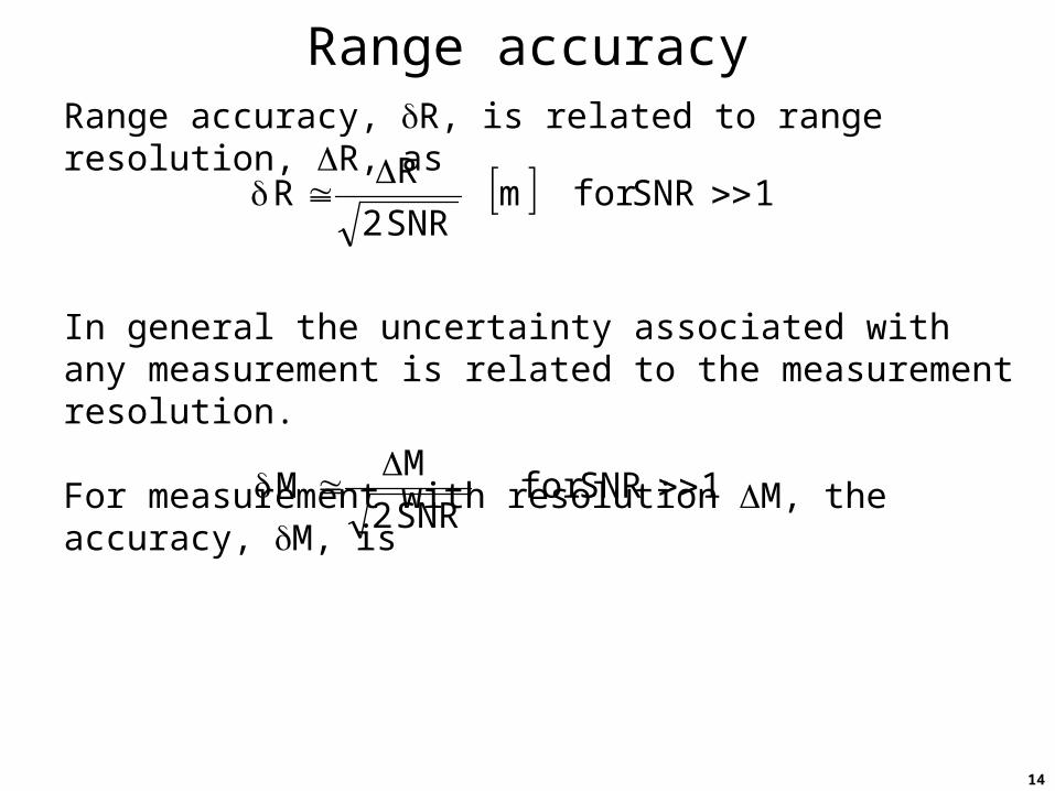
Range accuracyRange accuracy, R, is related to range resolution, R, as

In general the uncertainty associated with any measurement is related to the measurement resolution.

For measurement with resolution M, the accuracy, M, is

1SNRformSNR2

RR

1SNRforSNR2

MM

15

Analysis exampleTaken from problems 1.4 and 1.7 in the original textbook (solutions are found in Appendix V)

Consider the ACR 430 airfield-control radar for close control during aircraft approach in poor weather conditions.

This radar operates in the X band with f = 9.4 GHz.

The antenna measures 3.4 m horizontally and 0.75 m vertically.

The transmitter has peak output power, Pt, of 55 kW and a pulse

duration, , of 100 ns, (i.e., B = 10 MHz).

Radar system losses (L) total -5 dB and the received noise power, PN,

is -131 dBW.

For an aircraft RCS of 10 m2, find:

• the horizontal position error (range accuracy and az res) at 1 nautical mile

• the maximum range for aircraft detection (for SNR 13 dB)

16

Analysis examplePreliminary calculations

Wavelength, = c/9.4 GHz = 3.2 cm

Azimuth beamwidth, az = 0.032/3.4 = 9.4 mrad = 0.54 °

Elevation beamwidth, el = 43 mrad = 2.5 °

Gain, Gt = Gr = 4/(az el) = 31293 = 45 dBi

Range resolution, R = c / 2 = 15 m

Range accuracy, R = R / (2 SNR)

Azimuth resolution, R·az

1 nautical mile = 1852 m

R az = 1852 · 0.0094 = 17 m

17

Analysis exampleRange accuracy

need to find the SNR for R = 1852 m

SNR = Pt Gt Gr 2 L / [(4)3 R4 PN]

Pt (55 kW) 77 dBm

Gt·Gr 90 dBi

10 dBsm2 -30 dBsmL -5 dB

(4)-3 -33 dBR-4 -131 dB m4

PN-1 101 dBm

SNR79 dB or 80 106

Range accuracy, RR = R / (2 SNR) = 0.5 / (2 × 80 × 106) = 1 mm

The realizable range accuracy depends on the processing algorithm.

18

Analysis exampleNow find the range, Rmax, that results in a 13-dB SNR

Solving the radar range equation for R4 in terms of Pr yields

The received signal power required for a 13-dB SNR is

Pr(dB) = 13 + PN(dB) = -88 dBm

Therefore Rmax (dBm4) = 197

and Rmax = 84.1 km or 45 nautical miles

r3

2rtt4

P4

LGGPR

19

Design exampleFormation flying satellitesSystem requirements

position knowledge to within 3 mm (uncertainty)

range resolution of 15 cm (6 in)

Constraints

X-band operation (f = 10 GHz)

= 1 m2

maximum range, R = 20 km

antenna size, 1 m ×1 m

receiver noise figure, F = 2

T = 290 K

Loss, L = 0.5

Find

required bandwidth, B

required transmit power, Pt

20

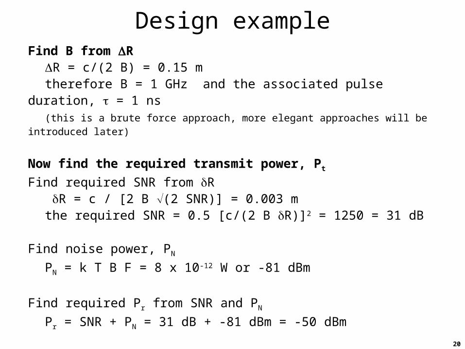
Design exampleFind B from R

R = c/(2 B) = 0.15 mtherefore B = 1 GHz and the associated pulse duration, = 1 ns(this is a brute force approach, more elegant approaches will be introduced later)

Now find the required transmit power, Pt

Find required SNR from R R = c / [2 B (2 SNR)] = 0.003 mthe required SNR = 0.5 [c/(2 B R)]2 = 1250 = 31 dB

Find noise power, PN

PN = k T B F = 8 x 10-12 W or -81 dBm

Find required Pr from SNR and PN

Pr = SNR + PN = 31 dB + -81 dBm = -50 dBm

21

Design exampleFind the gain of the antennas

Beamwidths, az = el = 0.03 rad = 1.7 °Gt = Gr = 4/(az el) = 14000 = 41 dBi

Find Pt using the radar range equation and required Pr

Gt·Gr 82 dBi

0 dBsm2 -30 dBsmL -3 dB(4)-3 -33 dBR-4 -172 dB m4

Pr /Pt -156 dB

Pr Pt – 156 dB = -50 dBm

Pt +106 dBm = 40 MWneed to get a 40-MW transmitter with a 1-ns pulse duration (non-trivial)

22

Doppler shift and velocityRelative motion between the radar’s antenna and the target produces a Doppler shift in the received signal frequency.

A simple derivationA target is located at a distance R [m] from a radar. The received electric field of the backscattered wave is given as

where E0 is the wave’s magnitude [V/m], t = 2ft [rad/s], k = 2/ [rad/m],

and is the wavelength of the transmitted wave [m].

The phase of the backscattered wave relative to its phase at R = 0 is

tj0

kR2tj0

tt eEeER,tE

]rad[R2

2Rk2

23

Doppler shift and velocityNow assume relative motion between the target and the radar such that the range, R, and phase, , change with time

Since frequency is the time derivative of phase, the received frequency differs from the transmitted frequency by the Doppler frequency shift, fD, (note: division by 2 to convert angular frequency to standard frequency)

or

where vr is the radial velocity [m/s].

td

Rd22

td

d

td

Rd2

td

d

2

1fD

]Hz[v2

f rD

24

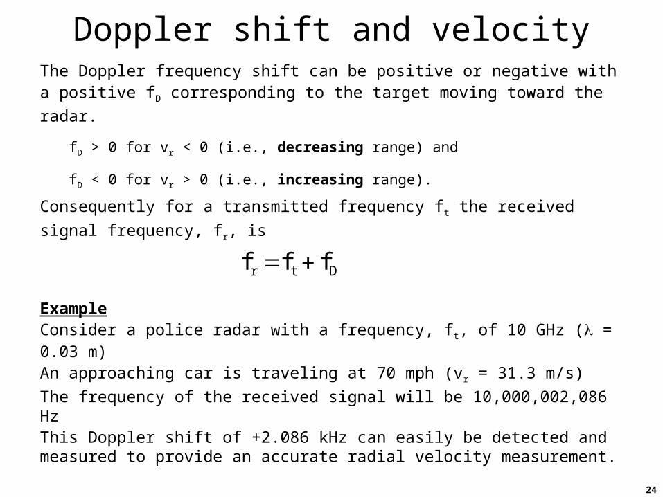
Doppler shift and velocityThe Doppler frequency shift can be positive or negative with a positive fD corresponding to the target moving toward the radar.

fD > 0 for vr < 0 (i.e., decreasing range) and

fD < 0 for vr > 0 (i.e., increasing range).

Consequently for a transmitted frequency ft the received signal

frequency, fr, is

ExampleConsider a police radar with a frequency, ft, of 10 GHz ( = 0.03 m)

An approaching car is traveling at 70 mph (vr = 31.3 m/s)

The frequency of the received signal will be 10,000,002,086 HzThis Doppler shift of +2.086 kHz can easily be detected and measured to provide an accurate radial velocity measurement.

Dtr fff

25

Doppler shift and velocityNow let’s focus on the radial velocity term.

Given the position, P, and velocity, v, both the radar and the target, the radial velocity and resulting Doppler frequency can be determined.

Therefore the Doppler frequency shift depends on

• relative velocity as seen from radar

• radar wavelength

Instantaneous position and velocity Relative velocity, v

Radial velocity component

vRadar

vTarget

v = vRadar - vTarget

vRadar vTarget

PRadarPTarget

RRadar path

Target path

vr = vR = v cos() [m/s]

fD = 2 v cos() / [Hz]

^v

R (unit vector)^ ^

=

vRadial = v R

vTangential

v

26

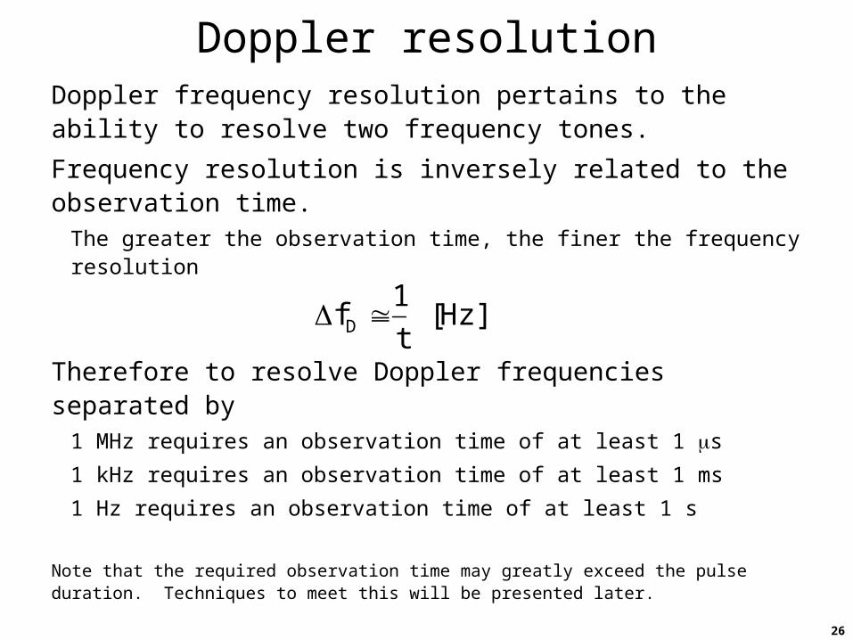
Doppler resolutionDoppler frequency resolution pertains to the ability to resolve two frequency tones.

Frequency resolution is inversely related to the observation time.

The greater the observation time, the finer the frequency resolution

Therefore to resolve Doppler frequencies separated by1 MHz requires an observation time of at least 1 s

1 kHz requires an observation time of at least 1 ms

1 Hz requires an observation time of at least 1 s

Note that the required observation time may greatly exceed the pulse duration. Techniques to meet this will be presented later.

]Hz[t

1fD

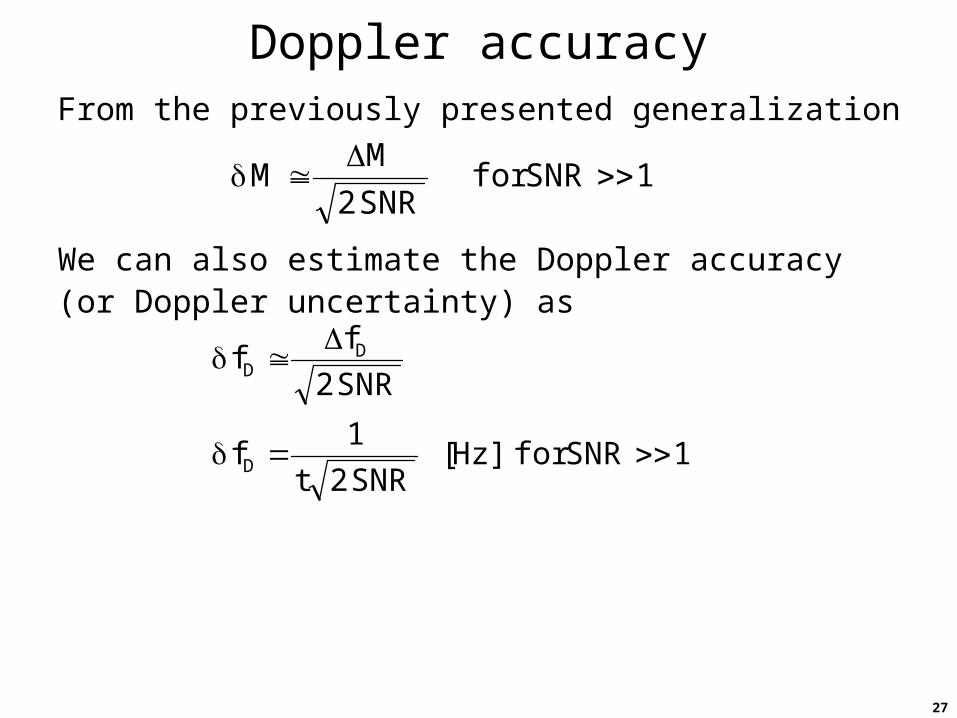
27

Doppler accuracyFrom the previously presented generalization

We can also estimate the Doppler accuracy (or Doppler uncertainty) as

1SNRforSNR2

MM

1SNRfor]Hz[SNR2t

1f

SNR2

ff

D

DD

28

Radial velocity resolution and accuracyThe radial velocity can be estimated from the measured Doppler frequency.

Similarly the radial velocity resolution and accuracy can be related to the Doppler resolution and accuracy.

Radial velocity resolution, vr

Radial velocity accuracy, vr

where t is the observation time

]s/m[2

fv D

r

]s/m[t22

fv D

r

1SNRfor]s/m[SNR2t22

fv D

r

29

Surveillance radar designPurpose: to detect and track ‘targets’ in the vicinity

Relevant to both military and civil applications

This is a ground-based appliction

The search space the entire sky (the upper hemisphere)

Generic system requirements Antenna considerations

All-weather operation L-band or S-band

Good angular position resolution large antenna

High-gain antennas (to reduce Pt) large antenna

Furthermore the search period should be dependent on the target dynamics

For example, for civil aircraft (sub-sonic speeds) a search period measured in 10s of seconds may be appropriate

30

Surveillance radar designThe antenna’s beamwidths (and hence gain) are related to the measurement rate as follows.

The upper hemisphere of the sky fills 2 sr of solid angle, sky

The antenna’s beam projects a solid angle ant = az el

Therefore the number of unique beam positions, NB, required to

search the sky is

Notice that NB = G/2. In general an antenna with gain G must probe G directions to

survey the 4 solid angle of an entire sphere (think spaceborne application)

Now given the search period, the dwell time, tdwell, (time

spent probing each beam position) is

elazant

skyB

2N

]s[N

periodsearcht

Bdwell

31

Surveillance radar designExample

Consider an application where T = 10 s and G = 36 dBi (4000).

Therefore the number of beam positions is NB = 2000 and

the dwell time is tdwell = 10/2000 = 5 ms.

So in those 5 ms the radar must detect any targets, measure the range to each it finds, and then repeat this process for the remaining 1999 beam positions over the next 9.995 seconds.

In addition the antenna beam must be essentially stationary, pointing at that piece of sky for those 5 ms and then switch instantly to the next position and so on. For a mechanically-steered antenna this may be quite a challenge, however electronically-steered antennas are available that can readily accomplish this.

32

Pulse repetition frequency (PRF)Continuing with the surveillance radar design, the focus now shifts to the timing of the transmit pulses and received echoes.

Issues include unambiguous range and velocity measurements

AssumptionsPulsed radar with periodic waveform transmission

No transmissions permitted during receive intervals (i.e., blind ranges)

Only one pulse in the air at a time (i.e., no pulses in the air during a Tx event)

Given the range to the most distant target of interest, Rmax, also known as the unambiguous range

We know that the minimum pulse period is 2Rmax/c

Therefore the maximum PRF is

]Hz[R2

c

periodpulse

1PRF

max

33

Pulse repetition frequency (PRF)Consider the case where a target at range 130 km is surveyed with a radar configured with a 100-km unambiguous range.

Rmax = 100 km, PRF = 1.5 kHz, 666-s pulse period

Round-trip travel time for 130-km target range

2R/c = 866 s

Ambiguous because unable to tell if echo pulse 2 results from Tx pulse A or B.

If echo 1 is from Tx A,then range is 30 km.

If echo 1 is from Tx B,the range is 130 km.

Therefore the radar has a 100-km range ambiguity.Possible solutions – discriminate between Tx pulses based on frequency, phase, polarization, pulse shape, etc.

34

Pulse repetition frequency (PRF)Another approach to resolving range ambiguities is to vary the PRF. (called PRF jitter or staggered PRF)

ExampleTarget range, R = 4050 m (2R/c = 27 s)

PRF1 = 50 kHz (PRI1 = 20 s)

PRF2 = 54 kHz (PRI2 = 18.5 s)

PRI (pulse repetition interval) = 1/PRF [s]

Also known as pulse repetition period (PRP), pulse repetition time (PRT), or inter-pulse period (IPP).

7 s.

8.5 s. time

Tx

Tx

Tx

Tx

Echoes from target at 4 km range 18.5 s.

20 s.

27 s.

54-kHz PRF

50-kHz PRF

35

Pulse repetition frequency (PRF)PRF and spatial sampling

Consider the case of an imaging radar where a moving radar illuminates a static scene

Most image formation algorithms require periodic radar samples to exploit efficient processing (e.g., fast-Fourier transforms, FFTs)

Non-periodic sampling significantly complicates this processing and is therefore discouraged.

Even the effects of a variable radar velocity can create problems leading some to slave the PRF to the radar’s ground speed to force a constant distance between samples, e.g., PRF = vground

Why don’t we simply use a lower PRF to avoid the range ambiguity problem entirely?

A lower PRF:

• reduces the number of observations within the dwell time

• affects the SNR if we can combining signals from multiple pulses

• creates Doppler measurement ambiguities

36

Pulse repetition frequency (PRF)Doppler ambiguities

The relative radial velocity produces a Doppler frequency shift.

For modest pulse durations (ns to s) the observation time is too short to resolve and accurately measure fD.

For a 1-s pulse duration, , (and a 1-s echo duration from a point target) the frequency resolution, f = 1/ = 1 MHz

Doppler frequencies of interest may be 10 to 1000 Hz, typically not MHz

Cannot arbitrarily increase pulse duration since the transmitter blinds the receiver creating a blind range, Rblind = c/2 [m] (Rblind = 150 m for = 1 s)

To overcome this limitation, signal phase information from successive pulses can be used for fD discrimination.

However to adequately sample fD, we must satisfy the Nyquist-

Shannon criterion which says that the sampling frequency, fs, must

exceed twice the signal’s bandwidth.B2fs

37

Doppler ambiguitiesTo unambiguously reconstruct a waveform, the Nyquist-Shannon sampling theorem (developed and refined from the 1920s to 1950s at Bell Labs) states that exact reconstruction of a continuous-time baseband signal from its samples is possible if the signal is bandlimited and the sampling frequency is greater than twice the signal bandwidth.

Application to radar means that the pulse-repetition frequency (PRF) must be at least twice the Doppler bandwidth.

For the case where the Doppler frequency shift will be 250 Hz (a 500-Hz Doppler bandwidth), the PRF must be at least 500 Hz.

Under this sampling plan we can only resolve signals with 250-Hz bandwidth and are hence unable to resolve + from – Doppler frequencies. However due to the predictable Doppler characteristics we are able to resolve + from – frequencies.

The lower PRF limit is determined by Doppler ambiguities

bandwidthDopplertheisf,f2PRF DDmin

38

PRF & Doppler ambiguities

39

PRF & Doppler ambiguitiesFailure to satisfy the Nyquist-Shannon requirement can lead to aliasing of undesired signals into the band of interest.

-1.2

-1

-0.8

-0.6

-0.4

-0.2

0

0.2

0.4

0.6

0.8

1

1.2

0 1 2 3 4 5time (ms)

Sig

nal

(V

)

400-Hz 600-Hz 1-kHz samples

-1.2

-1

-0.8

-0.6

-0.4

-0.2

0

0.2

0.4

0.6

0.8

1

1.2

0 1 2 3 4 5time (ms)

Sig

na

l (V

)

400-Hz 1-kHz samples

0 fsfs/2 fs/2

Digital domain spectrum

Analog domain spectrum

0

40

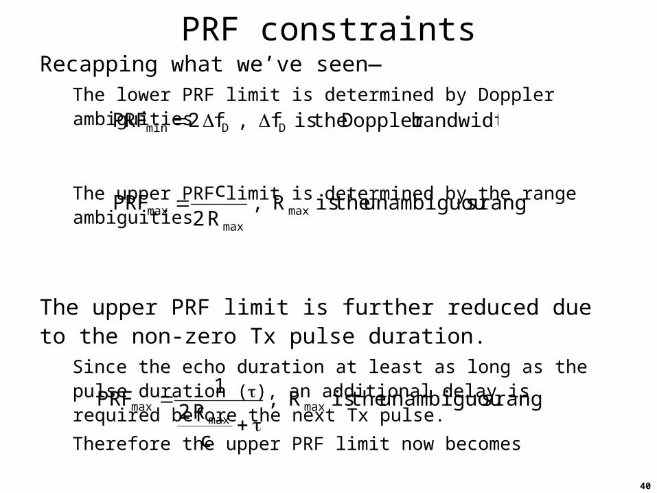
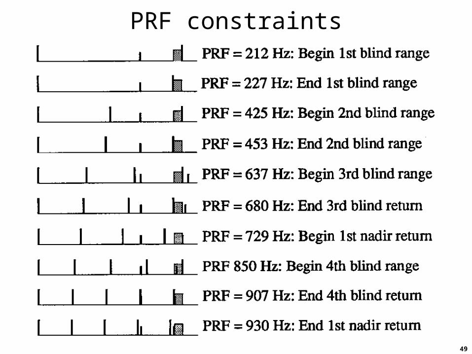
PRF constraintsRecapping what we’ve seen—

The lower PRF limit is determined by Doppler ambiguities

The upper PRF limit is determined by the range ambiguities

The upper PRF limit is further reduced due to the non-zero Tx pulse duration.

Since the echo duration at least as long as the pulse duration (), an additional delay is required before the next Tx pulse.

Therefore the upper PRF limit now becomes

bandwidthDopplertheisf,f2PRF DDmin

rangesunambiguoutheisR,R2

cPRF max

maxmax

rangesunambiguoutheisR,

cR2

1PRF max

maxmax

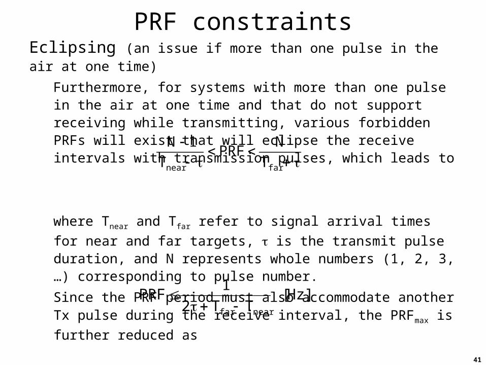
41

PRF constraintsEclipsing (an issue if more than one pulse in the air at one time)

Furthermore, for systems with more than one pulse in the air at one time and that do not support receiving while transmitting, various forbidden PRFs will exist that will eclipse the receive intervals with transmission pulses, which leads to

where Tnear and Tfar refer to signal arrival times for near and far

targets, is the transmit pulse duration, and N represents whole numbers (1, 2, 3, …) corresponding to pulse number.

Since the PRF period must also accommodate another Tx pulse during the receive interval, the PRFmax is further reduced as

farnear T

NPRF

T

1N

]Hz[TT2

1PRF

nearfar

42

PRF constraintsTx and Rx timing for airborne radar systems

Consider the case of an airborne radar system on a straight and level flight trajectory and an altitude h above a flat Earth.

Its antenna is oriented such that it illuminates a spot on the ground broadside to the aircraft effectively mapping a swath over time.

Given the altitude (h), the incidence angle (), and the elevation beamwidth (el), we can find the time of arrival for echo signals from

the swath.

where T1 = 2R1/c

Tx1

time

Txn+1Txn

T1 T2

h

el

0 x1 x2 xflat Earth swath width

R1

R2

R

echo from swath due to Tx1

43

PRF constraintsTx and Rx timing for airborne radar systems

Given the altitude, h = 10 km, the incidence angle = 25°, and the elevation beamwidth, el = 10°, we can find the distance from the ground track to the

near and far swath edges (x1, x2), the range to the near and far swath edges

(R1, R2) and the round-trip time of flight for echoes from the near and far

swath edges (T1, T2), the swath width, and the echo duration.

Tx1

time

Txn+1Txn

T1 T2

Find x1, R1, and T1

x1 = h tan( - el/2) = 3.64 km

R1 = h sec( - el/2) = 10.6 km

T1 = 2 R1/c = 70.9 s

Find x2, R2, and T2

x2 = h tan( + el/2) = 5.77 km

R2 = h sec( + el/2) = 11.5 km

T2 = 2 R2/c = 77 sFind the swath width and the echo duration

Swath width = x2 - x1 ≈ 2 km

Echo duration = T2 - T1 + = 6.1 s +

Therefore ignoring any guard time (e.g., for switches)

]Hz[s1.62

1PRF

Minimum period

2 + 6.1 s

h

el

0 x1 x2 xflat Earth swath width

R1

R2

R

44

Spherical Earth calculationsSpherical Earth geometry calculations

Re Earth’s average radius (6378.145 km)

h orbit altitude above sea level (km)

core angle

R radar range

look angle

i incidence angle

i

sin

R

sin

R

sin

hR e

i

e

coshRR2hRRR ee2

e2e

2

Re

Re

NadirPoint

h R

i

Radar Position

45

Spherical Earth calculationsSatellite orbital velocity calculations (for circular orbits)

Re Earth’s average radius (6378.145 km)

h orbit altitude above sea level (km)

v satellite velocity

vg satellite ground velocity

standard gravitational parameter (398,600 km3/s2 for Earth)

s/km,hRv e

hRRvv eeg

Re

hRfRn

swath

Radar VelocityAntenna pattern

46

Spherical Earth calculationsSwath width geometry calculations

Re Earth’s average radius (6378.145 km)

Rn range to swath’s near edge

Rf range to swath’s far edge

Wgr swath width on ground

Wr slant range swath width

n core angle to swath’s near edge

f core angle to swath’s far edge

i,m incidence angle at mid-beam

enfgr RW

nfr RRW

Re

Re

h Rf

n

f

Rn Wri,m

Wgr

m,igrr sinWW

47

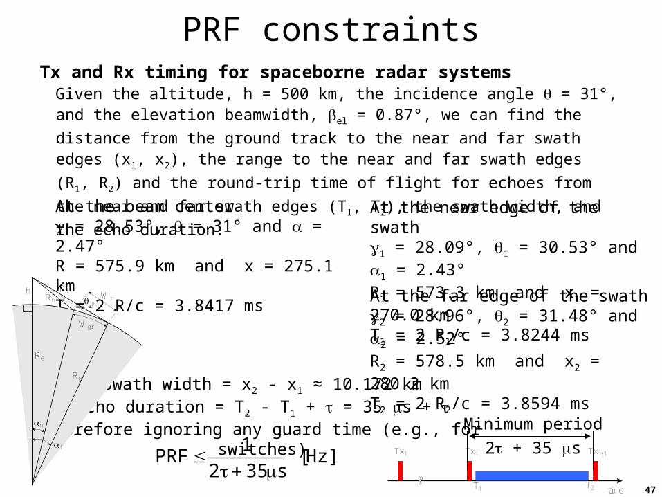
PRF constraintsTx and Rx timing for spaceborne radar systems

Given the altitude, h = 500 km, the incidence angle = 31°, and the elevation beamwidth, el = 0.87°, we can find the distance from the ground track to the

near and far swath edges (x1, x2), the range to the near and far swath edges

(R1, R2) and the round-trip time of flight for echoes from the near and far

swath edges (T1, T2), the swath width, and the echo duration.

Tx1

time

Txn+1Txn

T1 T2

At the beam center = 28.53°, = 31° and = 2.47°R = 575.9 km and x = 275.1 kmT = 2 R/c = 3.8417 ms

Swath width = x2 - x1 ≈ 10.172 kmEcho duration = T2 - T1 + = 35 s +

Therefore ignoring any guard time (e.g., for switches)

]Hz[s352

1PRF

Minimum period

2 + 35 s

Re

Re

h Rf

n

f

Rn Wri,m

Wgr

At the near edge of the swath1 = 28.09°, 1 = 30.53° and 1 = 2.43°R1 = 573.3 km and x1 = 270.0 kmT1 = 2 R1/c = 3.8244 ms

At the far edge of the swath2 = 28.96°, 2 = 31.48° and 2 = 2.52°R2 = 578.5 km and x2 = 280.2 kmT2 = 2 R2/c = 3.8594 ms

48

PRF constraints

49

PRF constraints

50

PRF constraints

51

Antenna length, velocity, and PRFGiven an antenna length, ℓ

wavelength,

velocity, v

We know

The Doppler bandwidth, BDop, is

Therefore PRFmin is

2

v22sin

v2fD

vvv

BDop

(small angle approximation)

v2B2PRF Dopmin

Note that PRFmin is independent of

Aircraft casev = 200 m/s, ℓ = 1 mPRFmin = 400 Hz

Spacecraft casev = 7000 m/s, ℓ = 10 mPRFmin = 1.4 kHz

fD < 0

ℓv

fD > 0

antenna

52

Receiver signal samplingAnalog-to-digital conversion

The analog-to-digital converter (ADC) plays a critical role in modern radar systems.

As was pointed out previously the ADC quantizes the analog video into discrete digital values

analog domain digital domain

Timing of sample conversion is controlled by ADC clockKey parameters of this process include:

• sampling frequency, fs

• ADC’s resolution NADC (i.e., the number of bits)

We will explore how each of these parameters relate to radar performance.

53

Sampling criteriaThe Nyquist-Shannon sampling theorem also applies to signal digitization in the analog-to-digital converter (ADC) requiring that the ADC sampling frequency be at least twice the waveform bandwidth.

For a signal with a 1-GHz bandwidth, the ADC’s sample rate must be at least 2 GHz (doable but non-trivial and expensive)

• The data acquisition system (ADC and associated control system and memory elements) will be expensive in terms of component cost, power dissipation, and complexity

• As digital switching speed increases, the power dissipation of the digital components increases

• High-speed ADC operation requires high-speed memory elements (RAM or FIFOs) with write-cycle time periods comparable to the sampling clock period

• Also high-speed data acquisition generally requires more memory depth than low-speed acquisition since the number of samples, Ns = fs echo duration

Example – a 2-GHz fs and a 10-s echo duration results in 20,000 samples

collected with a 500-ps sample period

54

Sampling criteriaOften radar receiver systems will use in-phase and quadrature signal processing (I and Q) wherein the received signal is decomposed into the equivalent of its real and imaginary components.

In these cases two ADCs are required to digitize these two representations of the received signal (bad – twice the complexity) but the sampling rate requirements on each ADC is reduced by half (good – easier)

90°Hybrid

LO

PowerSplitter

Rx signal

Filter

Filter

ADC

ADC

Inphase signal

Quadrature signal

ADC clock

55

Sampling criteriaReturning our attention to the Nyquist-Shannon sampling theorem, note that it means that the ADC sampling frequency be at least twice the waveform bandwidth for a bandlimited signal.

Thus for a baseband signal this requires the maximum signal frequency be less than or equal to 50% of the sampling frequency; hardware realization typically is more conservative due to challenges associated achieving a bandlimited signal.

Consider a baseband signal with spectral components from DC to 100 MHz. According to the Nyquist-Shannon theorem, a 200-MHz sampling frequency will suffice. To avoid severe requirements on the analog anti-aliasing filter that precedes the ADC (used to ensure a bandlimited signal) an additional margin will be added by requiring the maximum signal frequency to be 40% of fs, thus a 250-MHz sampling frequency might be used.

0 100 200 freq (MHz)fsfs/2

0 100 250 freq (MHz)fsfs/2

aliasing aliasing

Filter passband

Filter passband

56

Sampling criteriaAnd again returning to the Nyquist-Shannon sampling theorem, note that it means that the ADC sampling frequency be at least twice the waveform bandwidth for a bandlimited signal.

For an intermediate-frequency (IF) signal (not at baseband) theory requires a sampling frequency of at least twice the signal bandwidth. However aliasing issues may require a higher sampling frequency.

Consider an IF signal with 30 MHz of bandwidth and a 150-MHz center frequency. Per the Nyquist-Shannon theorem, the sampling frequency must be at least 60 MHz. However a 60-MHz sampling frequency will alias the signal upon itself thus irreparably distorting the signal.A higher sampling frequency of 120-MHz avoids this problem.

This technique is called undersampling.

150 freq (MHz)fsfs/2

aliasing

60

Filter passband

3fs/2 2fs 5fs/2 3fs0 150 freq (MHz)

fs/2

aliasing

120

Filter passband

3fs/2fs0 60

57

Undersampling

fs 2fs 3fsfs/2 3fs/2 5fs/2 7fs/2

Zone1

Zone2

Zone3

Zone4

Zone5

Zone6

Zone7

Zone8

0

58

Sampling criteriaSampling requirements

Finally, for a simple pulse system, with pulse duration , the sampling requirement is

For systems using more complex signal waveforms with bandwidth B, the sampling requirement is

2fs

B2fs

59

Sampling criteriaFast time and slow time

Radar systems sample the backscattered echo signal over two time scales.

This echo signal is sampled as it returns from a single transmit pulseSample start time is governed by the round-trip time of flight, speed of light

Sample frequency is driven by the signal bandwidth

This echo signal is sampled as the target moves relative to the radarSample start time is governed by the relative velocity, radar or target speed

Sample frequency is driven by the Doppler bandwidth

Therefore the radar simultaneously works in two time scales

Fast time – interval when the echo arrivessample period typically measured in ns or s

Slow time – interval between pulsessample period typically measured in ms to s

Signal processing (e.g., filtering) can be performed in either scale or axis.

Slow time

Fast tim

e

Radar data memory

60

ADC resolution and dynamic rangeThe ADC quantizes the analog input signal into a fixed number of bits, NADC, that is sometimes called the ADC’s

resolution.

This parameter is important in radar applications as it is related to the ADC’s dynamic range and thus affects the radar’s instantaneous dynamic range.

Dynamic range – the range of signal powers over which the signal is detectable and linear

The dynamic range’s lower limit is the minimum detectable signal which is related to the SNR.

The dynamic range’s upper limit is that power level that causes the receiver’s transfer function to become nonlinear (typically involving saturation).

61

ADC resolution and dynamic rangeThe radar’s dynamic range is determined by the dynamic range of several components in the receiver, both analog and digital.

The analog components (e.g., amplifiers, mixers, filters, switches, etc.) when properly designed will have a tremendous dynamic range (> 100 dB).

The primary digital component in this analysis is the analog-to-digital converter (ADC) whose dynamic range is set by the number of bits. Quite often the ADC’s dynamic range becomes the limiting factor affecting the radar’s dynamic range.

62

ADC resolution and dynamic rangeExample

Consider an 8-bit ADC has an analog input voltage range of 0 to 2 V.Eight bits of resolution provide 28 (or 256) possible states.The scale of the least significant bit (LSB) is 2 V/256 or 8 mV.

bit 0 1 2 3 4 5 6 7weight 8 mV 16 mV 32 mV 64 mV 128 mV 256 mV 512 mV 1024 mV

Therefore 000000002 = 00H = 0 V

111111112 = FFH = 2 V

Each next greater bit doubles the available voltage range.

Doubling (x2) of voltage range quadruples (x4) the power range (6 dB)

Therefore the ADC’s number of bits (NADC) sets the ADC’s dynamic range:

NADC (bits) 8 12 14 16

Dynamic rangeADC (dB)48 72 84 96

CLKD0

D1

D2

D3

D4

D5

D6

D7

LSB

MSB

8-bit parallel output

Analog-to-digital converter

VinAnalog voltage

Sample clock

dB6NRangeDynamic ADCADC

63

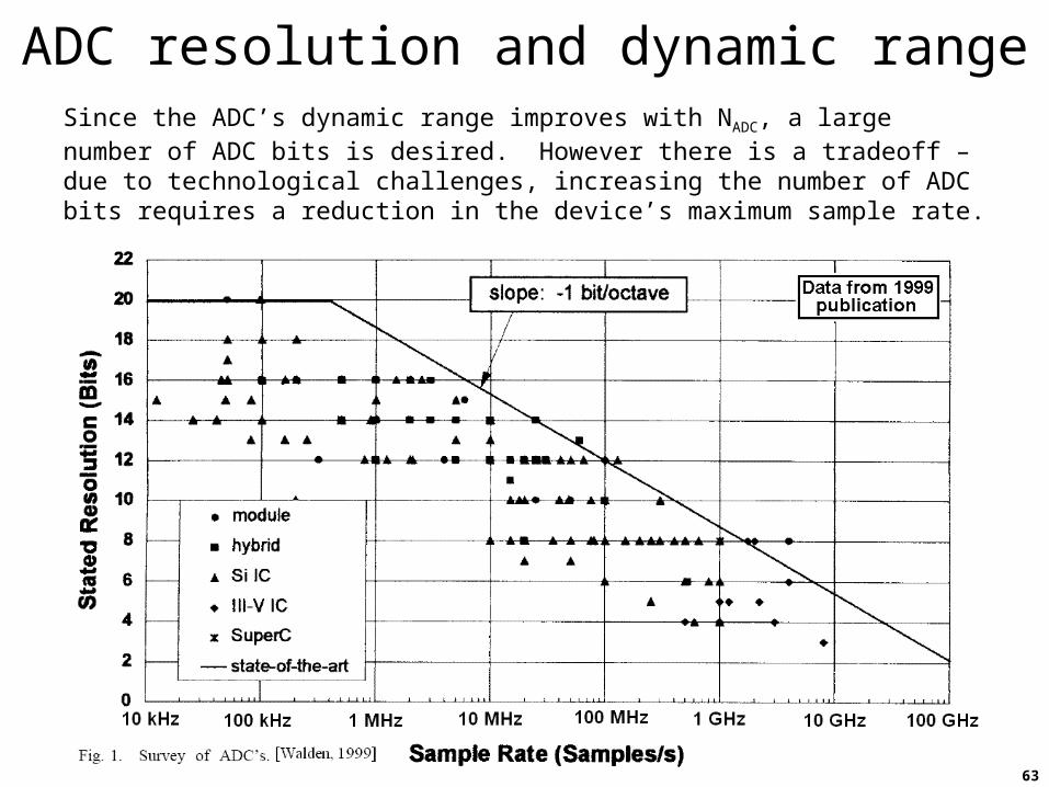
ADC resolution and dynamic rangeSince the ADC’s dynamic range improves with NADC, a large number of ADC bits is desired. However there is a tradeoff – due to technological challenges, increasing the number of ADC bits requires a reduction in the device’s maximum sample rate.

64

Dynamic rangeWhy is a large dynamic range so important?

Recall the ACR 430 airfield-control radar examplef = 9.4 GHz, PTx = 55 kW, = 100 ns, G = 45 dBi, PN = -101 dBm, Rmax = 84.1 km, R = 15 m, Rblind = 15 m

For a 10-m2 target RCS the received signal power is+ 2 dBm at a range of 800 m– 88 dBm at a range of 84.1 km (given as the minimum detectable signal)

+ 2 dBm – (– 88 dBm) = 90 dB

Therefore the system requires a 90-dB dynamic range to simultaneously accommodate echo signals from both near and distant targets.

This assumes all aircraft have a 10-dB RCS (not necessarily true) and ignores the possibility of jamming signals that might disrupt operation.A more conservative design might have a dynamic range > 95 dB

To provide a dynamic range greater than 95 dB requires an ADC with at least 16 bits of resolution.Based on 1999-era data, the fastest 16-bit ADC samples at a 3-MS/s rate but a 100-ns requires a 20-MS/s rate.

65

Dynamic rangeOne way to overcome this dynamic range problem is to recognize that the strong target echoes come from near targets whereas the weak target echoes come from distant targets and therefore reduce this predictable signal strength variation in the analog domain (before it gets to the ADC).

This technique of varying the receiver gain during the receive interval is known as swept gain or sensitivity time control (STC).It has the advantage of accommodating a large signal dynamic range with a limited instantaneous dynamic range.

Other techniques for accommodating a large signal dynamic range involve pulse compression and digital signal processing, topics yet to be covered.

fast time

Rx

po

wer

(d

B)

Rx

gai

n (

dB

)fast time

Vid

eo s

ign

al

po

wer

(d

B)

fast time

66

Data ratesThe rate at which data output from the ADC is another important system parameter, primarily this may represent a significant challenge to the signal processing, data transport, or data storage system.

The ADC output data flow at an uneven rate – between echoes the system is largely idle while during the echo acquisition time a burst of data flows.

Typically these data are buffered (e.g., in a FIFO) and read out at a slower pace to produce a steady data rate.

The data rate is determined by several radar system parameters

channelschannelsofnumbersample

bitsresolutionADC

channelsec

samplesratesamplesecdurationecho

sec

pulsesPRF

sec

bitsrateData

67

Data ratesExample

Consider a radar system with thefollowing parameters.

Pulse duration, = 1 sRmax = 50 km, PRF = 2 kHz

Echo duration = 350 sADC: fs = 1 MHz, NADC = 14 bits/channel, I & Q sample scheme (i.e., 2 channels)

The radar data rate, M, is

90°Hybrid

LO

PowerSplitter

Rx signal

Filter

Filter

ADC

ADC

Inphase signal

Quadrature signal

ADC clock

channels2sample

bits14channel/s/MS1s350kHz2

sec

bitsM

s/MB45.2s/Mb6.19M b: bits, B: bytes, 1 B = 8 b

Radar systems produce large data rates

68

Radar cross section (RCS)An object’s RCS depends on the characteristics

of the object (size, materials, geometry) and of the radar (frequency, polarization, orientation)

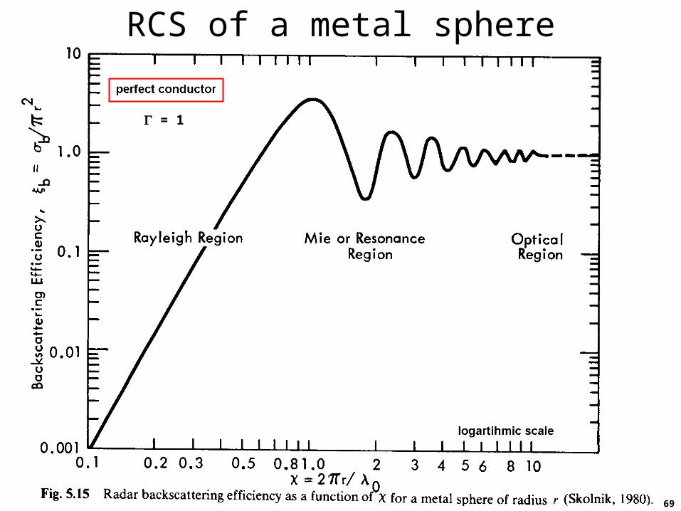
Consider the simple sphereThe RCS of a sphere is complex (although it is independent of

orientation due to its symmetry)

If the circumference is much larger than the wavelength (2r » )then RCS ≈ physical cross sectional area (r2) reflectivity (r, r)[called the optical region]

If the circumference is comparable to the wavelength (2r ) then RCS fluctuates with variations in size or wavelength[called the Mie region or resonance region]

If the circumference is much smaller than a wavelength (2r « ) then the RCS (r/)4

[called the Rayleigh region]

This explains why radars don’t typically ‘see’ air molecules and why the sky is blue.

69

RCS of a metal sphere

= 1

70

Radar cross section (RCS)The electrical properties of materials determine the reflection properties.

Electrical properties: , , , = (/)

For a smooth, planar, boundary between two half spaces with a plane wave incident normal to the surface, the reflection coefficient, R, is

The reflection coefficient, R, relates to field quantities (V/m).

Reflectivity, , relates to power (and RCS).

REEandR ir12

12

1, 1

2, 2

2

12

122R

71

Radar cross section (RCS)In many cases, 1 = 2 = o (= 4 10-7 H/m)

so that = o/r (where o = 377 ) and

Clearly approaches 1 for cases of high dielectric contrast (2/ 1) and

approaches 0 for cases of low contrast.

Example

Consider the three-layer structure composed ofair (r =1), ice (r = 3.2), and the bed.

Find the reflectivity at the two boundaries whenthe bed is rock (r =6) again when the bed is liquid water (r = 81)

0for

1

12

12

12

2

21

21

r1 1

r2 3.2

r3

air

ice

bed

air/ice

ice/bed

dB1108.0283.02.312.31 22

ice/air

dB16024.0156.088.1188.11 22

rock/ice

dB5.3447.0668.03.2513.251 22

water/ice

72

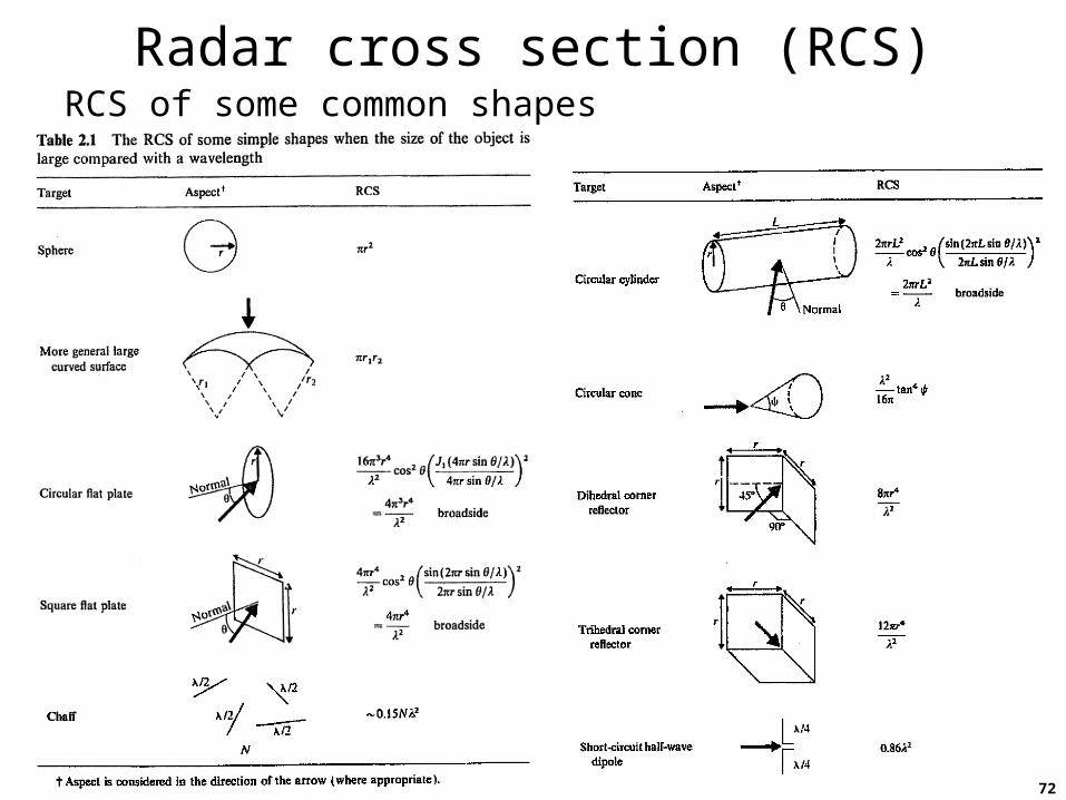
Radar cross section (RCS)RCS of some common shapes

73

Radar cross section (RCS)Dihedral and trihedral corner reflectors

74

Radar cross section (RCS)Dihedral and trihedral corner reflectors

75

Radar cross section (RCS)Luneberg lens

76

Radar cross section (RCS)Luneberg lens

77

Radar cross section (RCS)

78

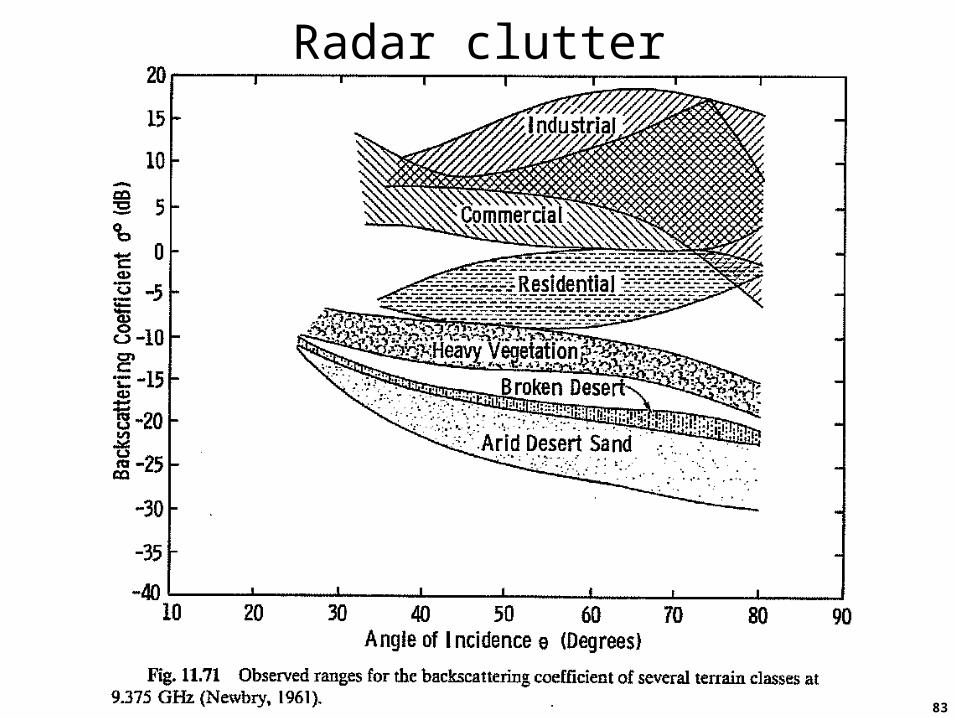
Radar clutterClutter: unwanted echoes from the environment

terrain, buildings, animals, aircraft, the ocean, rain, etc.

What is considered clutter depends on your applicationThree classes of clutter: point, surface, volume

Point: point targets

Surface: 2-D surface (e.g., ocean surface, cornfield)

Volume: 3-D volume (e.g., forest canopy, rain, snowpack)

CharacterizationPoint clutter: characterized by its RCS, [m2]

Surface clutter: characterized by its backscattering coefficient, [unitless] = c/Ac where c is average RCS of area Ac

Volume clutter: characterized by its volumetric backscatter, [m-1] = c/Vc where c is average RCS within volume Vc

79

Factors affecting backscatterThe backscattering characteristics of a surface are represented by the scattering coefficient,

For surface scattering, several factors affect Dielectric contrast

Large contrast at boundary produces large reflection coefficientAir (r = 1), Ice (r ~ 3.2), (Rock (4 r 9), Soil (3 r 10), Vegetation (2 r 15), Water (~ 80), Metal ( )

Surface roughness (measured relative to )RMS height and correlation length used to characterize roughness

Incidence angle, ()

Surface slopeSkews the () relationship

PolarizationVV HH » HV VH

]m[,p,p;,;, 2s0ss00

80

Surface roughness and backscatter

81

Surface roughness and backscatter

82

Backscatter from bare soil

Note: At 1.1 GHz, = 27.3 cm

83

Radar clutter

84

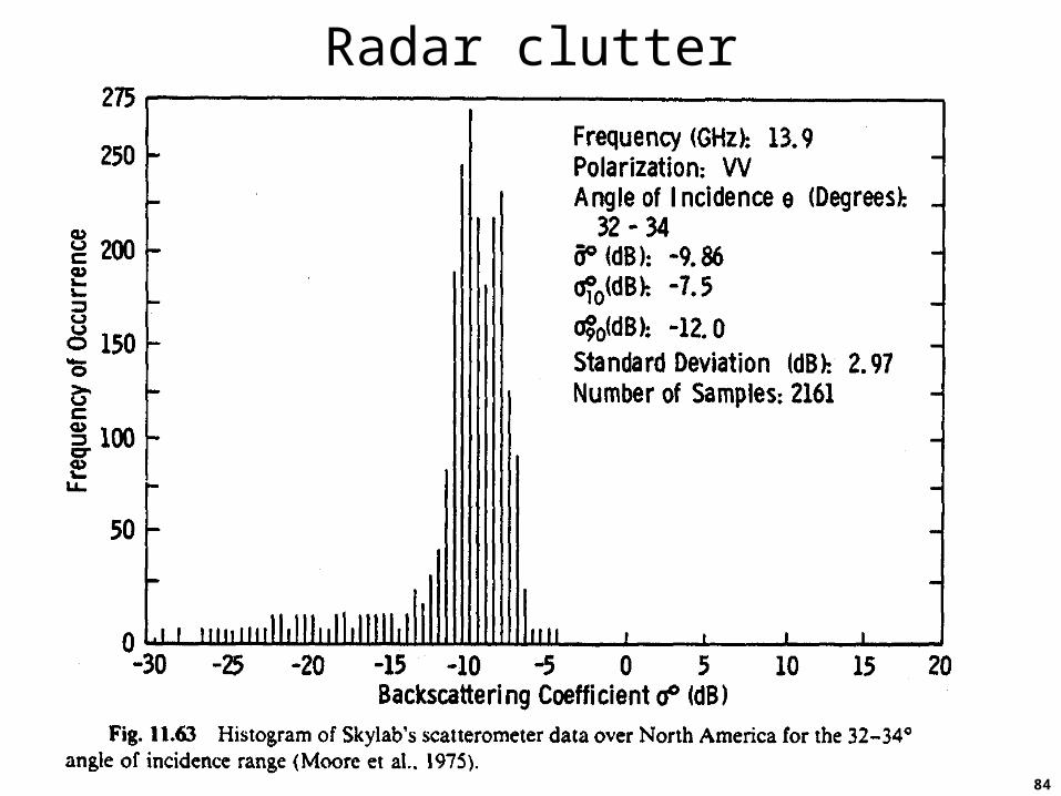
Radar clutter

85

Simple modelsFor purposes of radar system design, simple models for the backscattering characteristics from terrain can be used.

A variety of models have been developed.

Below are some of the more simple models that may be useful.

() = (0) cosn()

where is the incidence angle and n is a roughness-dependent variable.

n = 0 for a very rough (Lambertian) surface [() = (0)]

n = 1 for a moderately rough surface [() = (0) cos ()]

n = 2 for a moderately smooth surface [() = (0) cos2 ()]

() = (0) e-/ o

where is the incidence angle and o is a roughness-dependent angle.

In both model types (0) depends on the target characteristics

86

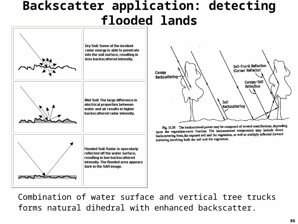
Backscatter application: detecting flooded lands

Combination of water surface and vertical tree trucks forms natural dihedral with enhanced backscatter.

87

Radar equation for extended targetsThe area of illumination to be used in the analysis is dependent on the system characteristics.

Different illumination areas result depending on whether the system is beam limited, pulse (or range) limited, Doppler (or speed) limited, or a combination of these.

88

Radar equation for extended targets

89

Radar equation for extended targetsFor homogeneous extended area targets (e.g., grass, bare soil, forest, water,

sand, snow, etc.) constant (though still dependent on , , and polarization).

Substituting this relationship leads to

where A is the system’s spatial resolution (A = x y) and

Pr is the mean value of the received signal power.

The scattering coefficient, , contains target information.Soil moisture

Surface wind speed and direction over water

Ground surface roughness

Water equivalent content of a snowpack

Therefore the accuracy and precision of measurements are important.

43

2t

2

rR4

AGPP

90

Ground imaging radarIn a real-aperture system images of radar backscattering are mapped into slant range, R, and along-track position.

The along-track resolution, y, is provided solely by the antenna. Consequently the along-track resolution degrades as the distance increases. (Antenna length, ℓ, directly affects along-track resolution.)

Cross-track ground range resolution, x, is incidence angle dependent

]m[Ry az

]m[sin2

cx p

where p is the compressed

pulse duration

y

xx

along-trackdirection

cross-trackdirection

cross-trackdirection

slant range

ground rangeground range

slant range