1

PSBS: Practical Size-Based SchedulingMatteo Dell’Amico, Damiano Carra, and Pietro Michiardi

Abstract—Size-based schedulers have very desirable performance properties: optimal or near-optimal response time can be coupledwith strong fairness. Despite this, however, such systems are rarely implemented in practical settings, because they require knowing apriori the amount of work needed to complete jobs: this assumption is difficult to satisfy in concrete systems. It is definitely more likelyto inform the system with an estimate of the job sizes, but existing studies point to somewhat pessimistic results if size-based policiesuse imprecise job size estimations.We take the goal of designing scheduling policies that explicitly deal with inexact job sizes. First, we prove that, in the absence oferrors, it is always possible to improve any scheduling policy by designing a size-based one that dominates it: in the new policy, no jobswill complete later than in the original one. Unfortunately, size-based schedulers can perform badly with inexact job size informationwhen job sizes are heavily skewed; we show that this issue, and the pessimistic results shown in the literature, are due to problematicbehavior when large jobs are underestimated. Once the problem is identified, it is possible to amend size-based schedulers to solvethe issue.We generalize FSP – a fair and efficient size-based scheduling policy – to solve the problem highlighted above; in addition, our solutiondeals with different job weights (that can be assigned to a job independently from its size). We provide an efficient implementation ofthe resulting protocol, which we call Practical Size-Based Scheduler (PSBS).Through simulations evaluated on synthetic and real workloads, we show that PSBS has near-optimal performance in a large variety ofcases with inaccurate size information, that it performs fairly and that it handles job weights correctly. We believe that this work showsthat PSBS is indeed pratical, and we maintain that it could inspire the design of schedulers in a wide array of real-world use cases.

F

1 INTRODUCTION

IN computer systems, several mechanisms can be modeledas queues where jobs (e.g., batch computations or data

transfers) compete to access a shared resource (e.g., pro-cessor or network). In this context, size-based schedulingprotocols, which prioritize jobs that are closest to comple-tion, are well known to have very desirable properties: theshortest remaining processing time policy (SRPT) providesoptimal mean response time [1], while the fair sojourn proto-col (FSP) [2] provides similar efficiency while guaranteeingstrong fairness properties.

Despite these characteristics, however, scheduling poli-cies similar to SRPT or FSP are very rarely deployed inproduction: the de facto standard are size-oblivious policiessimilar to processor sharing (PS), which divides resourcesevenly among jobs in the queue. A key reason is that, inreal systems, the job size is almost never known a priori. Itis, instead, often possible to provide estimations of job size,which may vary in precision depending on the use case;however, the impact of errors due to these estimations inrealistic scenarios is not yet well understood.

Perhaps surprisingly, very few works tackled the prob-lem of size-based scheduling with inaccurate job size in-formation: as we discuss more in depth in Section 2, theexisting literature gives somewhat pessimistic results, sug-gesting that size-based scheduling is effective only whenthe error on size estimation is small; known analyticalresults depend on restrictive assumptions on size estima-tions, while simulation-based analyses only cover a limitedfamily of workloads. More importantly, no study we areaware of tackled the design of size-based schedulers that areexplicitly designed with the goal of coping with errors in job size

• M. Dell’Amico and P. Michiardi are with EURECOM, France.• D. Carra is with University of Verona, Italy.

information. Our endeavor is to create a practical size-basedscheduling protocol, that has an efficient implementationand handles imprecise size information. In addition, thescheduler should allow setting weights to jobs, to control therelative proportion of the resources assigned to them.

In Section 3, we provide a proof that it is possible toimprove any size-oblivious policy by simulating that pol-icy and running jobs sequentially in the order in whichthey complete in the simulated policy. The resulting policydominates the latter: no job will complete later due to thepolicy change. This result generalizes the known fact thatFSP dominates PS [2] and gives strong fairness guarantees,but it does not hold when job size information is not exact.

In Section 4, we give a qualitative analysis of the im-pact of size estimation errors on scheduling behavior: weshow that, for heavy-tailed job size distributions, size-basedpolicies can behave problematically when large jobs areunder-estimated: this phenomenon, indeed, explains thepessimistic results observed in previous works.

Fortunately, it is possible to solve the aforementionedproblem: in Section 5, we propose a scheduling protocolthat drastically improves the behavior of disciplines such asFSP and SRPT when estimation errors exist. Our approach,which we call PSBS (Practical Size-Based Scheduler), is ageneralization of FSP featuring an efficient O(log n) imple-mentation and support for job weights.

We developed a simulator, described in Section 6, tostudy the behavior of size-based and size-oblivious schedul-ing policies in a wide variety of scenarios. Our simulatorallows both replaying real traces and generating syntheticones varying system load, job size distribution and inter-arrival time distribution; for both synthetic and real work-loads, scheduling protocols are evaluated on errors thatrange between relatively small quantities and others that

arX

iv:1

410.

6122

v4 [

cs.D

C]

6 A

ug 2

015

2

may vary even by orders of magnitude. The simulator isreleased as open-source software, to help reproducibility ofour results and to facilitate further experimentation.

From the experimental results of Section 7, we highlightthe following, validated both on synthetic and real traces:

1) When job size is not heavily skewed, SRPT and FSP out-perform size-oblivious disciplines even when job sizeestimation is very imprecise, albeit past work wouldhint towards important performance degradation; onthe other hand, when the job size distribution is heavy-tailed, performance degrades noticeably;

2) The scheduling disciplines we propose (from which wederive PSBS) do not suffer from the performance issuesof FSP and SRPT; they provide good performance for alarge part of the parameter space that we explore, be-ing outperformed by a processor sharing strategy onlywhen both the job size distribution is heavily skewedand size estimations are very inaccurate;

3) PSBS handles job weights correctly and behaves fairly,guaranteeing that most jobs complete in an amount oftime that is proportional to their size.

As we discuss in Section 8, we conclude that our workhighlights and solves a key weakness of size-based schedul-ing protocols when size estimation errors are present; thefact that PSBS consistently performs close to optimallyhighlights that size-based schedulers are more viable in realsystems than what was known from the state of the art; webelieve that our work can help inspiring both the designof new size-based schedulers for real systems and analyticresearch that can provide better insight on scheduling whenerrors are present.

2 RELATED WORK

We discuss two main areas of related work: first, resultsfor size-based scheduling on single-server queues whenjob sizes are known only approximately; second, practicalapproaches devoted to the estimation of job sizes.

2.1 Single-Server Queues

Performance evaluation of scheduling policies in single-server queues has been the subject of many studies inthe last 40 years. Most of these works, however, focus onextreme situations: the size of a given job is either completelyunknown or known perfectly. In the first (size-oblivious) case,smart scheduling choices can still be taken by consideringthe overall job size distribution: for example, in the commoncase where job sizes are skewed – i.e., a small percent-age of jobs are responsible for most work performed inthe system – it is smart to give priority to younger jobs,because they are likely to complete faster. Least-Attained-Service (LAS) [3], also known in the literature as Foreground-Background (FB) [4] and Shortest Elapsed Time (SET) [5],employs this principle. Similar principles guide the designof multi-level queues [6, 7].

When job size is known a priori, scheduling policiestaking into account this information are well known toperform better (e.g., obtain shorter response times) thansize-oblivious ones. Unfortunately, job sizes can often beonly known approximately, rather than exactly. Since in our

paper we consider this case, we review the literature thattargets this problem.

Perhaps due to the difficulty of providing analyticalresults, not much work considers the effect of inexact jobsize information on size-based scheduling. Lu et al. [8] havebeen the first to consider this problem, showing that size-based scheduling is useful only when job size evaluationsare reasonably good (high correlation, greater than 0.75,between the real job size and its estimate). Their evaluationfocuses on a single heavy-tailed job size distribution, anddoes not explain the causes of the observed results. Instead,we show the effect of different job size distributions (heavy-tailed, memoryless and light-tailed), and we show how tomodify the size-based scheduling policies to make themrobust to job estimation errors.

Wierman and Nuyens [9] provide analytical results fora class of size-based policies, but consider an impracticalassumption: results depend on a bound on the estimationerror. In the common case where most estimations are closeto the real value but there are outliers, bounds need to beset according to outliers, leading to pessimistic predictionson performance. In our work, instead, we do not imposeany bound on the error. Semi-clairvoyant scheduling [10, 11]is the problem where the scheduler, rather than knowingprecisely a job’s size s, knows its size class blog2 (s)c. It canbe regarded as similar to the bounded error case.

Other works examined the effect of imprecise size in-formation in size-based schedulers for web servers [12]and MapReduce [13]. In both cases, these are simulationresults that are ancillary to the proposal of a schedulerimplementation for a given system, and they are limitedto a single type of workload.

To the best of our knowledge, these are the only workstargeting job size estimation errors in size-based scheduling.We remark that, by using an experimental approach andreplaying traces, we can take into account phenomena thatare difficult to consider in analytic approaches, such asperiodic temporal patterns or correlations between job sizeand submission time.

2.2 Job Size Estimation

In the context of distributed systems, FLEX [14] andHFSP [15] proved that size-based scheduling can performwell in practical scenarios. In both cases, job size estimationis performed with very simple approaches (i.e., by samplingthe execution time of a part of the job): such rough estimatesare sufficient to provide good performance, and our resultsprovide an explanation to this.

In several practical contexts, rough job size estimationsare easy to perform. For instance, web servers can use filesize as an estimator of job size [16], and the variabilityof the end-to-end transmission bandwidth determines theestimation error. More elaborate ways to estimate size areoften available, since job size estimation is useful in manydomains; examples are approaches that deal with predictingthe size of MapReduce jobs [17, 18, 19] and of databasequeries [20]. Estimation error can be always evaluated aposteriori, and this evaluation can be used to decide if size-based scheduling works better than size-oblivious policies.

3

3 DOMINANCE RESULTS WITH KNOWN JOB SIZES

Friedman and Henderson have proven that FSP – a pol-icy that executes jobs serially in the order in which theycomplete in PS – dominates PS: when job sizes are knownexactly, no jobs complete later in PS than in FSP [2]. Thisis a strong fairness guarantee, but in most practical casesa policy such as FSP falls short because of its lack of con-figurability: for example, it does not allow to prioritize jobs.We show here that Friedman and Henderson’s results can begeneralized: no matter what the original scheduling policyis, it is possible to simulate it and execute jobs in the orderof their completion: the resulting policy will still dominateit. Our PSBS policy, described in Section 5, is an instance ofthis set of policies which allows setting job priorities.

We consider here the single-machine scheduling prob-lem with release times and preemption. In this section,we consider the offline scheduling problem, where releasetimes and sizes of each job are known in advance. As weshall see in the following, PSBS (like FSP) guarantees thesedominance results while also being appliable online, i.e.,without any information about jobs released in the future.

Our goal, that materializes in the Pri scheduler, is tominimize the sum of completion times (using Graham etal.’s notation [21], the 1|ri; pmtn|

∑Ci problem) with the

additional dominance requirement: no job should completelater than in a scheduler which is taken as a reference forfairness. Without this limitation, the optimal solution is theShortest Remaining Processing Time (SRPT) policy. We callschedule a function ω (i, t) that outputs the fraction of systemresources allocated to job i at time t. For example, for theprocessor-sharing (PS) scheduler, when n jobs are pending(released and not yet completed), ω (i, t) = 1

n if job i ispending and 0 otherwise. Furthermore, we call Ci,ω thecompletion time of job i under schedule ω.

Definition 1. Schedule ω dominates schedule ω′ if Ci,ω ≤Ci,ω′ for each job i.

Our scheduler prioritizes jobs according to the order inwhich they complete in ω: its completion sequence.

Definition 2. A completion sequence S = [s1, . . . , sn] is anordering of the jobs to be scheduled. A schedule ω hascompletion sequence S if Csi,ω ≤ Csj ,ω∀i < j.

Definition 3. For a completion sequence S, the PriS sched-ule is such that PriS (i, t) = 1 if i is the first pending job toappear in S; PriS (i, t) = 0 otherwise.

We now show that scheduling jobs in the order in whichthey complete under ω′ dominates ω.

Theorem. PriS dominates any schedule with completion se-quence S.

Proof. We have to show that Ci,PriS ≤ Ci,ω for each job iand any schedule ω with completion sequence S. Let j bethe position of i in S (i.e., i = sj); we call M the minimalmakespan of the S≤j = s1, . . . , sj set of jobs,1 and weshow that Ci,PriS ≤M and M ≤ Ci,ω :

1. The makespan of a set of jobs is the maximum among their comple-tion times, therefore M = minω∈Ω maxi∈1,...,j CSi,ω where Ω is theset of all possible schedules.

• Ci,PriS ≤M : minimizing the makespan of S≤j is equiv-alent to solving the 1|ri; pmtn|Cmax problem appliedto the jobs in S≤j : this is guaranteed if all resourcesare assigned to jobs in S≤j as long as any of them arepending [22]. PriS guarantees this, hence the makespanof S≤j using PriS is M . Since i ∈ S≤j , Ci,PriS ≤M .

• M ≤ Ci,ω follows trivially from ω having completionsequence S and, therefore, Ci,ω being the makespan forS≤j using schedule ω.

This theorem generalizes Friedman and Henderson’sresults: FSP follows from applying PriS to the completionsequence of PS. The generalization is important: in practice,one can define a scheduler that provides a desired type offairness, and optimize the performance in terms of comple-tion time by applying the PriS scheduler. If the system dealswith different classes of jobs that have different weights,we can take discriminatory processor sharing (DPS) as areference: our theorem guarantees that PriS dominates DPS.We have exploited exactly this results in our PSBS scheduler,which, in the absence of errors, dominates DPS. Only whenerrors are present – and this dominance result does notapply – PSBS deviates from the behavior of PriS .

4 SCHEDULING BASED ON ESTIMATED SIZES

We now describe the effects that estimation errors haveon existing size-based policies such as SRPT and FSP. Wenotice that under-estimation triggers a behavior which isproblematic for heavy-tailed job size distributions: this isthe key insight that will lead to the design of PSBS.

4.1 SRPT and FSPSRPT gives priority to the job with smallest remainingprocessing time. It is preemptive: a new job with size smallerthan the remaining processing time of the running one willpreempt (i.e., interrupt) the latter. When the scheduler hasaccess to exact job sizes, SRPT has optimal mean sojourntime (MST) [1] – sojourn time, or response time, is the timethat passes between a job’s submission and its completion.

SRPT may cause starvation (i.e., never providing access toresources): for example, if small jobs are constantly submit-ted, large jobs may never get served; while this phenomenonappears rare in practical cases [23], it is nevertheless wor-rying. FSP (also known as fair queuing [24] and Vifi [25])doesn’t suffer from starvation by virtue of job aging: FSPserves the job that would complete earlier in a virtual em-ulated system running a processor sharing (PS) discipline:since all jobs eventually complete in the virtual system, theywill also eventually be scheduled in the real one.

With no estimation errors, FSP provides a value of MSTwhich is close to what is provided by SRPT while guar-anteeing fairness due to the dominance result discussedin Section 3. When errors are present, this property is notguaranteed; however, our results in Section 7.5 show thatFSP preserves better fairness than SRPT also in this case.

4.2 Dealing With Errors: SRPTE and FSPEWe now consider SRPT and FSP when the scheduler usesestimated job sizes rather than exact ones. For clarity, we willrefer hereinafter to SRPTE and FSPE in this case.

4

Over-estimation

t

t

t

t

Rem

aini

ng si

ze

Rem

aini

ng si

ze

Rem

aini

ng si

ze

Rem

aini

ng si

ze

J1 J2

J3

J2

J3

J1 ^

J4

J5 J6

J4 J5

J6 ^

Under-estimation

Fig. 1. Examples of scheduling without (top) and with (bottom) errors.

In Fig. 1, we provide an illustrative example where asingle job size is over- or under-estimated while the othersare estimated correctly, focusing (because of its simplicity)on SRPTE; sojourn times are represented by the horizontalarrows. The left column of Fig. 1 illustrates the effect of over-estimation. In the top, we show how the scheduler behaveswithout errors, while in the bottom we show what happenswhen the size of job J1 is over-estimated. The graphs showsthe remaining (estimated) processing time of the jobs overtime, assuming a normalized service rate of 1. Withouterrors, J2 does not preempt J1, and J3 does not preemptJ2. Instead, when the size of J1 is over-estimated, both J2and J3 preempt J1. Therefore, the only penalized job (i.e.,experiencing higher sojourn time) is the over-estimated one.Jobs with smaller sizes are always able to preempt an over-estimated job, therefore the basic property of SRPT (favoringsmall jobs) is not significantly compromised.

The right column of Fig. 1 illustrates the effect of under-estimation. With no estimation errors (top), a large job, J4, ispreempted by small ones (J5 and J6). If the size of the largejob is under-estimated (bottom), its estimated remainingprocessing time eventually reaches zero: we call late a jobwith zero or negative estimated remaining processing time.A late job cannot be preempted by newly arrived jobs, sincetheir size estimation will always be larger than zero. Inpractice, since preemption is inhibited, the under-estimatedjob monopolizes the system until its completion, impactingnegatively all waiting jobs.

This phenomenon is particularly harmful with heavilyskewed job sizes, if estimation errors are proportional tosize: if there are few very large jobs and many small ones,a single late large job can significantly delay several smallones, which will need to wait for the late job to complete foran amount of time which is disproportionate to their sizebefore having an opportunity of being served.

Even if the impact of under-estimation seems straight-forward to understand, surprisingly no work in the literaturehas ever discussed it. To the best of our knowledge, we are thefirst to identify this problem, which significantly influences

scheduling policies dealing with inaccurate job size.In FSPE, the phenomena we observe are analogous:

job size over-estimation delays only the over-estimated job;under-estimation can result in jobs terminating in the virtualPS queue before than in the real system; this is impossiblein absence of errors due to the dominance result introducedin Section 4.1. We therefore define late jobs in FSPE as thosewhose execution is completed in the virtual system but notyet in the real one and we notice that, analogously to SRPTE,also in FSPE late jobs can never be preempted by new ones,and they block the system until they are all completed.

5 OUR SOLUTION

Now that we have identified the issue with existing size-based scheduling policies, we propose a strategy to avoidit. It is possible to envision strategies that update job sizeestimations as work progresses in an effort to reduce errors;such solutions, however, increase the complexity both indesigning systems and in analyzing them. In fact, the effec-tiveness of such a solution would depend non-trivially onthe way size estimation errors evolve as jobs progress: this isinextricably tied to the way estimators are implemented andto the application use case. We propose, instead, a solutionthat requires no additional job size estimation, based on theintuition that late jobs should not prevent executing other ones.This goal is achievable with simple modifications to pre-emptive size-based scheduling disciplines such as SRPT andFSP; the key property is that the scheduler takes correctiveactions when one or more jobs are late, guaranteeing thatnewly arrived small jobs will execute soon even when verylarge late jobs are running.

We conclude this section by showing our proposal,PSBS; it implements this idea while being efficient (O(log n)complexity) and allowing the usage of different weightsto differentiate jobs. Our experimental results show thatPSBS achieves almost optimal mean sojourn times for alarge variety of workloads, suggesting that more complexsolutions involving re-estimations are unlikely to be verybeneficial in many practical cases.

5.1 Using PS and LAS for Late Jobs

From our analysis of Section 4.2, we understand that currentsize-based schedulers behave problematically when one ormore jobs become late. Fortunately, it is possible to under-stand if jobs are late from the internal state of the scheduler:in SRPT, a job is late if its remaining estimated size is lessthan or equal to zero; in FSP, a job is late if it is completedin the virtual time but not in the real time.

As outlined above, approaches that involve job size re-estimation are difficult to design and evaluate, especiallyfrom the point of view of this work, where we do not makeany assumption on the job size estimators; our approach,therefore, requires only one size estimation per job.

The key idea of our proposal is that late jobs should notmonopolize the system resources. The solution is to modifythe scheduler such that it provides service to a set of jobs,which we call eligible jobs, rather than a single job at a time.In particular, we consider the following jobs as eligible whenat least one job is late: for our amended version of SRPTE, all

5

the late jobs, plus the non-late job with the highest-priority;for our amended version of FSPE, only the late jobs.

The two cases differ because, in SRPTE, jobs only becomelate while they are being served since remaining processingtime decreases only for them; therefore, non-late jobs needa chance to be served. We serve only one non-late job tominimize unnecessary deviations from SRPTE. In FSPE,conversely, jobs become late depending on the simulatedbehavior of the virtual time, independently from which jobsare served in the real time.

We take into account two choices for scheduling eligiblejobs: PS and LAS (see Section 2.1). PS divides resourcesevenly between all jobs, while LAS divides resources evenlybetween the job(s) that received the least amount of serviceuntil the current time.

The alternatives proposed so far lead to four schedulingpolicies that we evaluate experimentally in Section 7:

1) SRPTE+PS. Behaving as SRPTE as long as no jobs arelate, switching to PS between all late jobs and thehighest-priority non-late job;

2) SRPTE+LAS. As above, but using LAS instead of PS;3) FSPE+PS. Behaving as FSPE as long as no jobs are late,

switching to PS between all late jobs;4) FSPE+LAS. As above, but using LAS instead of PS.

We point out that, in the absence of errors or just of sizeunderestimations, jobs are guaranteed to be never late; thismeans that in such cases these scheduling policies will beequivalent to SRPT(E) and FSP(E), respectively. For a moreprecise description, we point the interested reader to theirimplementation in our simulator.2

5.2 PSBSIn Section 7.1 we show how the scheduling protocols wepropose outperform, in most cases, both existing size-basedscheduling policies and size-oblivious ones such as PS andLAS. Betweeen the scheduling protocols just introduced, wepoint out that FSPE+PS is the only one that guaranteesto avoid starvation: every job will eventually complete inthe virtual time, and therefore will be scheduled in a PSfashion. Conversely, both SRPTE and LAS can starve largejobs if smaller ones are continuously submitted. Due to thisproperty and to the good performance we observe in theexperiments of Section 7.2, we consider FSPE+PS a desirablepolicy. It has, however, a few shortcomings: first, it doesnot handle weights to differentiate job priorities; second, itsimplementation is inefficient, requiring O(n) computationwhere n is the number of jobs running in the emulated sys-tem. Here, we propose PSBS, a generalization of FSPE+PSwhich solves these problems, both allowing different jobweights and having an efficient O(log n) implementation.

5.2.1 Job WeightsNeither FSP nor PS support job differentiation through jobweights. In particular, FSP schedules jobs based on theircompletion time in a virtual time that simulates an envi-ronment using PS, which treats all running jobs equally.

To differentiate jobs in PSBS, we use DiscriminatoryProcessor Sharing (DPS) [26] in the place of PS, both in

2. https://github.com/bigfootproject/schedsim/blob/4745b4b581029c4f9cbbb791f43386d32d0ef8f6/schedulers.py

virtual time

Rem

aini

ng v

irtua

l siz

e J1

J2

J3

t = 0 (g = 0)

t = 3 (g = 3)

t = 5 (g = 4)

t = 11 (g = 6)

t = 15 (g = 8)

t = 17 (g = 10)

s1 = 10 g1 = 10 s2 = 5

g2 = 8 s3 = 2 g3 = 6

Fig. 2. Example of virtual time t and virtual lag g, used for sorting jobs.

the virtual time and in the scheduling for late jobs. DPS is ageneralization of PS whereby each job is given a weight,and resources are shared between processes proportionallyto their weight. By assigning a different weight to jobs, wecan therefore prioritize important jobs. When all weightsare the same, DPS is equivalent to PS; when each job has thesame weight PSBS is equivalent to FSPE+PS.

Our handling of weights follows classic algorithms likeWeighted Fair Queuing (WFQ) and Weighted Round Robin(WRR), accelerating aging (i.e., the decrease of virtual size)proportionally to weight, so that jobs with higher weight arescheduled earlier. Our result from Section 3 guarantees thatPSBS dominates DPS if job sizes are known exactly, whileat the same time being an online scheduler, implementedwithout any knowledge of jobs released in the future.

5.2.2 ImplementationFSP emulates a virtual system running a processor sharing(PS) discipline and keeps track of its job completion order;FSP then schedules one job at a time following that order.Whenever a new job arrives, FSP needs to update the re-maining size of each job in the emulated system to computethe new virtual finish times and the corresponding jobcompletion order. Existing implementations of FSP [2, 27]have O(n) complexity due to the job virtual remaining sizeupdate at each arrival.

In our implementation, we reduce the complexity ofthe update procedure. Before showing the details of thealgorithm, we introduce an example to help understandour solution. Consider three jobs (J1, J2 and J3) withsizes s1 = 10, s2 = 5 and s3 = 2 respectively, weightsw1 = w2 = w3 = 1, which arrive at times t = 0, t = 3and t = 5 respectively. Fig. 2 shows the evolution of thevirtual emulated system, i.e., how the remaining virtual sizedecreases in the virtual time. For instance, when job J3arrives, since it will complete in the virtual time before jobsJ1 and J2, it will be executed immediately in the real system(job J2 will be preempted). To compute the completion time,it is possible to calculate the exact virtual remaining size ofthe jobs currently in the system.

We instead introduce a new variable, which we callvirtual lag g. The key idea is that we store, for each job i,

6

a job virtual lag gi so that i completes in the virtual time whenthe virtual lag g = gi. We fulfill this property by updating gat a rate that depends on the number of jobs in the system:for each time unit in the virtual time, g increases by 1/wv ,where wv is the sum of the weights wi of each job i runningin the virtual emulated system.

Given a job i with weight wi and size si that arrives atthe system when the virtual lag g has a value g = x, the jobvirtual lag is given by gi = x + si/wi. The job virtual laggi is computed just once, when the job arrives, and it doesnot need to be updated when other jobs arrive. In fact, onlythe global virtual lag g needs to be updated according to thenumber of jobs in the system. Fig. 2 shows the job virtuallag computed when each jobs arrives (value of gi below si)and the value of the global virtual lag g (below the virtualtime t). Indeed, each job i completes when g = gi, but theonly variable we update at each job arrival is g, leavinguntouched the values gi of the job virtual lags. For instance,when job J3 arrives, the virtual lag g has value 4, thereforethe job virtual lag will be g3 = 4 + 2 (since the size andthe weights of job J3 are s3 = 2 and w3 = 1). It takes 6time units (in the virtual time) to complete job J3, whichcorresponds to 2 time units in the virtual lag.

It is simple to show that, given any positive value forsi and wi, the order at which jobs complete in the virtualtime and in the virtual lag is exactly the same. Therefore, ateach job arrival, it is sufficient to update the global virtuallag g, compute the job virtual lag gi and store the object ina priority queue, where the order is kept according to thevalues of gi. The overall complexity is dominated by themaintenance of the priority queue, which is O(log n), sinceit is not necessary to update the virtual remaining size of alljobs in the system to compute the completion order.

The implementation of our solution, shown in Algo-rithm 1, follows the nomenclature used in the originaldescription of FSP [2, Section 4.4]. We remark that, in theabsence of errors and when all job weights are the same,PSBS is equivalent to FSP: therefore, our implementation ofPSBS is also the first O(log n) implementation of FSP.

Computation is triggered by three events: if a job iof weight wi and estimated size si arrives at time t,JobArrival(t, i, si, wi) is called; when a job i completes,RealJobCompletion(i) is called; finally, when a job completesin virtual time at time t, VirtualJobCompletion(t) is called(NextVirtualCompletionTime is used to discover when tocall VirtualJobCompletion). After each event, ProcessJob iscalled to determine the new set of scheduled jobs: its outputis a set of (j, s) pairs where j is the job identifier and s is thefraction of system resources allocated to it.

As auxiliary data structures, we keep two priorityqueues, O and E . O stores jobs that are running both in thereal time and in the virtual time, while E stores “early” jobsthat are still running in the virtual time but are completedin the real time. For each job i, we store in O or E animmutable tuple (i, gi, wi) containing respectively the job id,the virtual lag gi and the weight. We use binary min-heapsto represent O and E , using the gi values as ordering key:binary heaps are efficient data structures offering worst-case O(log n) “push” and “pop” operations, O(1) lookup ofthe first value and eassentially optimal memory efficiency,by virtue of being an implicit data structure requiring no

”””Set up the scheduler state.O and E contain (i, gi, wi) tuples: i is the job id, gi isthe value of g at which the job completes in the virtualtime and wi is the weight. They are sorted by gi. ”””

def Init:g ← 0 # virtual lag (see text)t← 0 # virtual time# virtual time queueO ← empty binary min-heap# “early” jobs completed in real timeE ← empty binary min-heap# mapping from job ids of late jobs to their weightL ← empty hashtablewL ← 0 #

∑wi for each late job i

wv ← 0 #∑wi∀i running in virtual time

def NextVirtualCompletionTime:if O and/or E are not empty:

g ← minfirst gi in O,first gi in Ereturn t+ wv(g − g)

else: return ∅

def UpdateVirtualTime(t):if wv > 0: g ← g + (t− t)/wvt← t

def VirtualJobCompletion(t):UpdateVirtualTime(t)if first gi in O ≤ g:

(i, , wi)← pop(O)L[i]← wiwL ← wL + wi

else: # the virtual job that completes is in E( , , wi)← pop(E)

wv ← wv − wi

def RealJobCompletion(i):if L is not empty: # we were scheduling late jobs

wi ← pop(L[i])wL ← wL − wi

else: # we were scheduling the first job in Opush pop(O) into E

def JobArrival(t, i, si, wi):UpdateVirtualTime(t)push (i, g + si/wi, wi) into Owv ← wv + wi

def ProcessJob:if L is not empty: return (i, wi/wL) : (i, wi) ∈ Lelif O is not empty: return (first job id of O, 1)else: return ∅

Algorithm 1: PSBS.

pointers [28]. In addition, the push operation has of O(1)complexity on average [29]. The state of the scheduler iscompleted by a mapping L from the identifiers of late jobsto their weight, a counter t representing the virtual time, andtwo variables wv and wL representing the sum of weightsfor jobs that are respectively active in the virtual time and

7

late. Some additional bookkeeping, not included here forsimplicity, would be needed to handle jobs that completeeven when they are not scheduled (e.g., because of errorconditions or after being killed): we refer the interestedreader to the implementation in our simulator.3 Additionaldetails can be found in the supplemental material.

Complexity Analysis: We consider here averagecomplexity due to the worst-case O(n) complexity ofhashtable operations.4 It is trivial to see that NextVirtual-CompletionTime and UpdateVirtualTime have O(1) com-plexity. Since inserting elements in hashtables has O(1)average complexity, the cost of VirtualJobCompletion isdominated by the pop operations on O and E : both of themare bound by O(log n), where n is the number of jobs in thesystem. Removing an element from a hashtable has O(1)average cost, so the cost of RealJobCompletion is dominatedby the pop on O, which has again O(log n) complexity.JobArrival has O(1) average complexity (remember thatpushing elements on a binary heap is O(1) on average).

The ProcessJob procedure, when L is not empty, hasO(|L|) complexity because the output itself has size L.This is however very unlikely to be a limitation in prac-tical cases, since real-world implementations of schedulersallocate resources one by one in discrete slots: schedulerssuch as PS or DPS are abstractions of mechanisms suchas round-robin or max-min fair schedulers, which can beimplemented efficiently; a real-world implementation ofPSBS would adopt similar strategy to mimick the DPS-likeresource sharing when L is not empty. We also note that,when there are no job size estimation errors and PSBS isused to implement FSP, L is guaranteed to always be emptyand therefore ProcessJob will have O(1) complexity.

As we have seen, with the exclusion of ProcessJob asdiscussed above, all the procedures of the scheduler have atmost O(log n) computational complexity. Coupled O(log n)operations having low constant factors because they areimplemented on binary heaps, which are very efficient datastructures, we believe that these performance guaranteesare sufficient for a very large set of practical situations: forexample, CFS – the current Linux scheduler – has O(log n)complexity since it uses a tree structure [31].

6 EVALUATION METHODOLOGY

Understanding size-based scheduling when there are esti-mation errors is not a simple task; analytical studies havebeen performed only with strong assumptions such asbounded error [9]. Moreover, to the best of our knowledge,the only analytical result known for FSP (without estimationerrors) is its dominance over PS, making analytical com-parisons between SRPTE-based and FSPE-based schedulingpolicies even more difficult.

For these reasons, we evaluate our proposals throughsimulation. The simulative approach is extremely flexible,allowing to take into account several parameters – distribu-tion of the arrival times, of the job sizes, of the errors. Pre-vious simulative studies (e.g., [8]) have focused on a subset

3. https://github.com/bigfootproject/schedsim/blob/4745b4b581029c4f9cbbb791f43386d32d0ef8f6/schedulers.py

4. A denial-of-service attack on hashtables has been designed byforging keys to obtain collisions [30]. This attack is defeated in modernimplementations by salting keys before hashing.

of these parameters, and in some cases they have used realtraces. In our work, we developed a tool that is able to bothreproduce real traces and generate synthetic ones. Moreover,thanks to the efficiency of the implementation, we were ableto run an extensive evaluation campaign, exploring a largeparameter space. For these reasons, we are able to providea broad view of the applicability of size-based schedulingpolicies, and show the benefits and the robustness of oursolution with respect to the existing ones.

6.1 Scheduling Policies Under Evaluation

In this work, we take into account different schedulingpolicies, both size-based and size-oblivious. For the size-based disciplines, we consider SRPT as a reference forits optimality with respect to the MST. When introducingthe errors, we evaluate SRPTE, FSPE and our proposalsdescribed in Section 5.

As size-oblivious policies, we have implemented theFirst In, First Out (FIFO) and Processor Sharing (PS) dis-ciplines, along with DPS, the generalization of PS withweights [6]. These policies are the default disciplines usedin many scheduling systems – e.g., the default schedulerin Hadoop [32] implements a FIFO policy, while Hadoop’sFAIR scheduler is inspired by PS; the Apache web serverdelegates scheduling to the Linux kernel, which in turn im-plements a PS-like strategy [16]. Since PS scheduling dividesevenly the resources among running jobs, it is generallyconsidered as a reference for its fairness (see the next sectionon the performance metrics). Finally, we consider also theLeast Attained Service (LAS) [3] policy. LAS scheduling isa preemptive policy that gives service to the job that hasreceived the least service, sharing it equally in a PS mode incase of ties. LAS scheduling has been designed consideringthe case of heavy-tailed job size distributions, where a largepercentage of the total work performed in the system is dueto few very large jobs, since it gives higher priority to smalljobs than what PS would do.

6.2 Performance Metrics

We evaluate scheduling policies according to two mainaspects: mean sojourn time (MST) and fairness. Sojourn time isthe time that passes between the moment a job is submittedand when it completes; such a metric is widely used inthe scheduling literature. The definition of fairness is moreelusive: in his survey on the topic, Wierman [33] affirmsthat “fairness is an amorphous concept that is nearly impossibleto define in a universal way”. When the job size distributionis skewed, it is intuitively unfair to expect similar sojourntimes between very small jobs and much larger ones; acommon approach is to consider slowdown, i.e. the ratiobetween a job’s sojourn time and its size, according to theintuition that the waiting time for a job should be somewhatproportional to its size. In this work we focus on the per-jobslowdown, to check that as few jobs as possible experience“unfair” high slowdown values; moreover, in accordancewith Wierman’s definition [34], we also evaluate conditionalslowdown, which evaluates the expected slowdown given ajob size, verifying whether jobs of a particular size experi-ence an “unfair” high expected slowdown value.

8

Parameter Explanation Defaultsigma σ in the log-normal error distribution 0.5shape shape for Weibull job size distribution 0.25timeshape shape for Weibull inter-arrival time 1njobs number of jobs in a workload 10,000load system load 0.9

TABLE 1Simulation parameters.

6.3 Parameter Settings

We empirically evaluate scheduling policies in a wide spec-trum of cases. Table 1 synthetizes the input parameters ofour simulator; they are discussed in the following.

Job Size Distribution: Job sizes are generated ac-cording to a Weibull distribution, which allows us to evalu-ate both heavy-tailed and light-tailed job size distributions.The shape parameter allows to interpolate between heavy-tailed distributions (shape < 1), the exponential distri-bution (shape= 1), the Raleigh distribution (shape = 2)and light-tailed distributions centered around the ‘1’ value(shape > 2). We set the scale parameter of the distribution toensure that its mean is 1.

Since scheduling problems have been generally analyzedon heavy-tailed workloads with job sizes using distributionssuch as Pareto, we consider a default heavy-tailed case ofshape = 0.25. In our experiments, we vary the shape param-eter between a very skewed distribution with shape = 0.125and a light-tailed distribution with shape = 4.

Size Error Distribution: We consider log-normallydistributed errors. A job having size s will be estimated ass = sX , where X is a random variable with distribution

Log-N (0, σ2). (1)

This choice satisfies two properties: first, since error ismultiplicative, the absolute error s− s is proportional to thejob size s; second, under-estimation and over-estimation areequally likely, and for any σ and any factor k > 1 the (non-zero) probability of under-estimating s ≤ s

k is the same ofover-estimating s ≥ ks. This choice also is substanciatedby empirical results: in our implementation of the HFSPscheduler for Hadoop [15], we found that the empirical errordistribution was indeed fitting a log-normal distribution.

The sigma parameter controls σ in Equation 1, with adefault – used if no other information is given – of 0.5; withthis value, the median factor k reflecting relative error is1.40. In our experiments, we let sigma vary between 0.125(median k is 1.088) and 4 (median k is 14.85).

It is possible to compute the correlation between theestimated and real size as σ varies. In particular, when sigmais equal to 0.5, 1.0, 2.0 and 4.0, the correlation coefficient isequal to 0.9, 0.6, 0.15 and 0.05 respectively.

The mean of this distribution is always larger than 1,and, as sigma grows, the system is biased towards over-estimating the aggregate size of several jobs, limiting theunderestimation problems that our proposals are designedto solve. Even in this setting, the results in Section 7 showthat the improvements we obtain are still significant.

Job Arrival Time Distribution: For the job inter-arrival time distribution, we use again a Weibull distributionfor its flexibility to model heavy-tailed, memoryless and

light-tailed distributions. We set the default of its shapeparameter (timeshape) to 1, corresponding to “standard”exponentially distributed arrivals. Also here, timeshapevaries between 0.125 (very bursty arrivals separated by longintervals) and 4 (regular arrivals).

Other Parameters: The load parameter is the meanarrival rate divided by the mean service rate. As a default,we use 0.9 like Lu et al. [8]; in our experiments we let itvary between 0.5 and 0.999. The number of jobs (njobs)in each simulation round is 10,000. For each experiment,we perform at least 30 repetitions, and we compute theconfidence interval for a confidence level of 95%. For veryheavy-tailed job size distributions (shape ≤ 0.25), resultsare very variable and therefore, to obtain stable averages,we performed hundreds and/or thousands of experimentruns, at least until the confidence levels have reached the5% of the estimated values.

7 EXPERIMENTAL RESULTS

We now proceed to an extensive report of our experimentalfindings. We first provide a high-level view showing thatour proposals outperform PS, excepting only extreme casesof both error and job skew (Section 7.1); we then proceed to amore in-depth comparison of our proposals, to validate ourchoice of using FSPE+PS as a base for PSBS (Section 7.2).We then evaluate the performance of PSBS against existingschedulers, while varying the two parameters that mostinfluence scheduler performance: shape (Section 7.3) andsigma (Section 7.4). We proceed to show that PSBS handlesjobs fairly (Section 7.5) and that job weights are handledcorrectly (Section 7.6); we conclude our analysis on syntheticworkloads by showing that our results hold even whilevarying settings over the parameter space (Section 7.7).We conclude our analysis by comparing PSBS to existingschedulers on real workloads extracted from Hadoop logsand an HTTP cache (Section 7.8).

For the results shown in the following, parameterswhose values are not explicitly stated take the default valuesin Table 1. For readability, we do not show the confidenceintervals: for all the points, in fact, we have performed anumber of runs sufficiently high to obtain a confidenceinterval smaller than 5% of the estimated value. Wherenot otherwise stated, all the wi parameters representing theweight of each job i have always been set to 1.

7.1 Mean Sojourn Time Against PS

We begin our analysis by comparing the size-based schedul-ing policies, using PS as a baseline because PS and itsvariants are the most widely used set of scheduling policiesin real systems. In Fig. 3 we plot the value of the MSTobtained using SRPTE, FSPE and the four alternatives wepropose in Section 5.1, normalizing it against the MST ofPS. We vary the sigma and shape parameters influencingrespectively job size distribution and error rate; we willsee that these two parameters are the ones that influenceperformance the most. Values lower than one (below thedashed line in the plot) represent regions where size-basedschedulers perform better than PS.

9

shape

0.125 0.25 0.5 12

4

sigma

0.1250.25

0.51

24

MST

/M

ST(P

S)

0.250.51248163264128

(a) SRPTE.

shape

0.125 0.25 0.5 12

4

sigma

0.1250.25

0.51

24

MST

/M

ST(P

S)

0.250.51248163264128

(b) SRPTE+PS.

shape

0.125 0.25 0.5 12

4

sigma

0.1250.25

0.51

24

MST

/M

ST(P

S)

0.250.51248163264128

(c) SRPTE+LAS.

shape

0.125 0.25 0.5 12

4

sigma

0.1250.25

0.51

24

MST

/M

ST(P

S)

0.250.51248163264128

(d) FSPE.

shape

0.125 0.25 0.5 12

4

sigma

0.1250.25

0.51

24

MST

/M

ST(P

S)

0.250.51248163264128

(e) FSPE+PS.

shape

0.125 0.25 0.5 12

4

sigma

0.1250.25

0.51

24

MST

/M

ST(P

S)

0.250.51248163264128

(f) FSPE+LAS.

Fig. 3. Mean sojourn time against PS: the dashed line is the boundary where MST is equivalent to that of PS. We recall that a low shape value isassociated to high job size skew, while high sigma entails imprecise job size estimates.

In accordance to intuition and to what is known fromthe literature, we observe that the performance of size-based scheduling policies depends on the accuracy of jobsize estimation: as sigma grows, performance suffers. Inaddition, from Figures 3a and 3d, we observe a new phe-nomenon: job size distribution impacts performance even morethan size estimation error. On the one hand, we notice thatlarge areas of the plots (shape > 0.5) are almost insensitiveto estimation errors; on the other hand, we see that MSTbecomes very large as job size skew grows (shape < 0.25).We attribute this latter phenomenon to the fact that, as wehighlight in Section 4, late jobs whose estimated remaining(virtual) size reaches zero are never preempted. If a largejob is under-estimated and becomes late with respect to itsestimation, small jobs will have to wait for it to finish inorder to be served.

As we see in Figures 3b, 3c, 3e and 3f, our proposals outper-form PS in a large class of heavy-tailed workloads where SRPTEand FSPE suffer. The net result is that the size-based policieswe propose are outperformed by PS only in extreme caseswhere both the job size distribution is extremely skewed andjob size estimation is very imprecise.

It may appear surprising that, when job size skew isnot extreme, size-based scheduling can outperform PS evenwhen size estimation is very imprecise: even a small cor-relation between job size and its estimation can direct thescheduler towards choices that are beneficial on aggregate.In fact, as we see more in detail in the following (Section 7.3),sub-optimal scheduling choices become less penalized asthe job size skew diminishes.

7.2 Comparing Our Proposals

How do the schedulers we proposed in Section 5.1 compare?In Fig. 4 we examine the empirical cumulative distributionfunction (ECDF) of the slowdown for all jobs we simulatewhile varying the shape parameter (sigma maintains itsdefault value of 0.5); we plot the results for PS as a referenceand observe that the staircase-like pattern observable inFig. 4a is a clustering around integer values obtained if asmall job gets submitted while n larger ones are running.

We observe that, in general, our proposals pay off: forall values of shape considered, the slowdown distributionof our proposals is well lower than the one of PS. Wealso observe a difference between the schedulers based onSRPTE and those based on FSPE: a noticeably larger numberof jobs experience an optimal slowdown of 1 when usinga scheduler based on FSPE. This is because, when usingFSPE-based scheduling policies, the number of jobs that areeligible for PS- or LAS-based scheduling is higher: whenlate jobs exist, only they are eligible to be scheduled, unlikewhat happens in SRPTE-based policies; as a consequence,several small jobs suffer in SRPTE-based policies becausethey are preempted too aggressively: as soon as they becomelate, even if they are the only late job in the system. Thisconfirms the soundness of the design policy we adopted inSection 5.1: minimizing the number of eligible jobs for PS-or LAS-based scheduling. Fig. 4 shows that even allowingto schedule a single non-late job can hurt performance.

Since the number of late jobs is generally small, differ-ences in scheduling between FSPE+PS and FSPE+LAS arerare. This is confirmed by noticing that the lines for the twoschedulers in Fig. 4 are essentially analogous; we conclude

10

100 101

slowdown

0.0

0.2

0.4

0.6

0.8

1.0EC

DF

FSPE+PSFSPE+LASSRPTE+PS

SRPTE+LASPS

(a) shape = 0.25.

100 101

slowdown

0.0

0.2

0.4

0.6

0.8

1.0

ECD

F

FSPE+PSFSPE+LASSRPTE+PS

SRPTE+LASPS

(b) shape = 1.

100 101

slowdown

0.0

0.2

0.4

0.6

0.8

1.0

ECD

F

FSPE+PSFSPE+LASSRPTE+PS

SRPTE+LASPS

(c) shape = 4.

Fig. 4. Distribution of per-job slowdown. The two FSPE-based policies perform best, with negligible differences between them.

0.125 0.25 0.5 1 2 4shape

2

4

6

8

10

MST

/M

ST(S

RPT

) SRPTEFSPEPSBS

PSLASFIFO

Fig. 5. Impact of shape. PSBS behaves close to optimally in all cases.

that FSPE+PS and FSPE+LAS have essentially analogousperformance. This fact and the property that FSPE+PSavoids starvation, as noted in Section 5.2, motivated us todevelop PSBS as a generalization of FSPE+PS.

7.3 Impact of Shape

After validating the choice of PSBS as a generalization ofFSPE+PS, we now examine how it performs when comparedto the optimal MST that SRPT obtains. In the followingFigures, we show the ratio between the MST obtained withthe scheduling policies we implemented and the optimalone of SRPT, while fixing sigma to its default value of 0.5.

From Fig. 5, we see that the shape parameter is fun-damental for evaluating scheduler performance. We noticethat PSBS has almost optimal performance for all shape valuesconsidered, while SRPTE and FSPE perform poorly for highlyskewed workloads. Regarding non size-based policies, PSis outperformed by LAS for heavy-tailed workloads (shape< 1) and by FIFO for light-tailed ones having shape > 1;PS provides a reasonable trade-off when the job size dis-tribution is unknown. When the job size distribution isexponential (shape = 1), non size-based scheduling policiesperform analogously; this is a result which has been provenanalytically (see e.g. the work by Harchol-Balter [35] and thereferences therein). It is interesting to consider FIFO: in it,jobs are scheduled in series, and job priority is not correlatedwith size: indeed, the MST of FIFO is equivalent to theone of a random scheduler executing jobs in series [36].FIFO can be therefore seen as the limit case for a size-basedscheduler such as FSPE or SRPTE when estimations carry noinformation at all about job sizes; the fact that errors becomeless critical as skew diminishes can be therefore explainedwith the similar patterns observed for FIFO.

7.4 Impact of SigmaThe shape of the job size distribution is fundamental indetermining the behavior of scheduling algorithms, andheavy-tailed job size distributions are those in which the be-havior of size-based scheduling differs noticeably. Becauseof this, and since heavy-tailed workloads are central in theliterature on scheduling, we focus on those.

In Fig. 6, we show the impact of the sigma parameterrepresenting error for three heavily skewed workloads. Inall three plots, the values for FIFO fall outside of the plot.These plots demonstrate that PSBS is robust with respectto errors in all the three cases we consider, while SRPTEand FSPE suffer as the skew between job sizes grows. Inall three cases, PSBS performs better than PS as long assigma is lower than 2: this corresponds to lax bounds onsize estimation quality, requiring a correlation coefficientbetween job size and its estimate of 0.15 or more.

In all three plots, PSBS performs better than SRPTE; thedifference between PSBS and FSPE, instead, is discernibleonly for shape < 0.25. We explain this difference by notingthat, when several jobs are in the queue, size reduction inthe virtual queue of FSPE is slow: hence, less jobs becomelate and therefore non preemptable. As the distributionbecomes more heavy-tailed, more jobs become late in FSPEand differences between FSPE and PSBS become significant,reaching differences of even around one order of magnitude.

In particular in Fig. 6b, there are areas (0.5 < sigma < 2)in which increasing errors decreases (slightly) the MST ofFSPE. This counterintuitive phenomenon is explained bythe characteristics of the error distribution: the mean of thelog-normal distribution grows as sigma grows, thereforethe aggregate amount of work for a set of several jobs ismore likely to be over-estimated; this reduces the likelihoodthat several jobs at once become late and therefore non-preemptable. In other words, FSPE works better with esti-mation means that tend to over-estimate job size; however, itis always better to use PSBS, which provides a more reliableand performant solution to the same problem.

In additional experiments – not included due to spacelimitations – we observed similar results with other errordistributions; in cases where errors tend towards underes-timations, we find that the improvements that PSBS givesover FSPE and SRPTE are even more important.

7.5 FairnessWe now consider fairness, intending – as discussed in Sec-tion 6.2 – that jobs’ running time should be proportional totheir size, and therefore slowdowns should not be large.

11

0.125 0.25 0.5 1 2 4sigma

2

4

6

8

10M

ST/

MST

(SR

PT) SRPTE

FSPEPSBS

PSLAS

(a) shape = 0.25

0.125 0.25 0.5 1 2 4sigma

1

10

100

MST

/M

ST(S

RPT

) SRPTEFSPEPSBS

PSLAS

(b) shape = 0.177

0.125 0.25 0.5 1 2 4sigma

1

10

100

1000

MST

/M

ST(S

RPT

) SRPTEFSPEPSBS

PSLAS

(c) shape = 0.125

Fig. 6. Impact of error on heavy-tailed workloads, sorted by growing skew.

10−4 10−3 10−2 10−1 100 101 102

job size

100

101

102

103

104

105

106

107

slow

dow

n

SRPTEFSPEPSBS

PSLASFIFO

Fig. 7. Mean conditional slowdown. PSBS outperforms PS, the sched-uler often taken as a reference for fairness.

Conditional Slowdown: To better understand thereason for the unfairness of FIFO, SRPTE and FSPE, in Fig. 7we evaluate mean conditional slowdown, showing averageslowdown (job sojourn time divided by job size) against jobsize, using our default simulation parameters. The figurehas been obtained by sorting jobs by size and binningthem into 100 job classes having similar size and containingthe same number of jobs; points plotted are obtained byaveraging job size and slowdown in each of the 100 classes.

The lines of FIFO, SRPTE and FSPE are almost parallelfor smaller jobs because, below a certain size, job sojourntime is essentially independent from job size: indeed, it dependson the total size of older (for FIFO) or late (for SRPTE andFSPE) jobs at submission time.

We confirm experimentally that the expected slowdownin PS is constant, irrespectively of job size [34]; PSBS andLAS, on the other hand, have close to optimal slowdownfor small jobs. PSBS has a better MST because it performsbetter for larger jobs, which are more penalized in LAS.

Per-Job Slowdown: Our results testify that, for PSBSand similarly to LAS, slowdown values are homogeneousacross classes of job sizes: neither small nor big jobs arepenalized when using PSBS. This is a desirable result, butthe reported results are still averages: to ensure that sojourntime is commensurate to size for all jobs, we need to investi-gate the per-job slowdown distribution.

In Fig. 8, we plot the CDF of per-job slowdown for ourdefault parameters. By serving efficiently smaller jobs, size-based scheduling techniques and LAS manage to obtainan optimal slowdown of 1 for most jobs. However, somejobs experience very high slowdown: those with slowdownlarger than 100 are around 1% for FSPE and around 8% forSRPTE. PS, LAS, and PSBS perform well in terms of fairness,with no jobs experiencing slowdown higher than 100 in

100 101 102

slowdown

0.0

0.2

0.4

0.6

0.8

1.0

ECD

F SRPTEFSPEPSBS

PSLASFIFO

100 101 102

slowdown

0.90

0.92

0.94

0.96

0.98

1.00

ECD

F

Fig. 8. Per-job slowdown: full CDF (top) and zoom on the 10% morecritical cases (bottom).

our experiment runs.5 While PS is generally considered thereference for a “fair” scheduler, it obtains slightly betterslowdown than LAS and PSBS only for the most extremecases, while being outperformed for all other jobs.

7.6 Job WeightsWe now consider how PSBS handles job weights. We con-sider workloads generated with all the default values shownin Table 1. Since we are not aware of representative work-loads where job priorities and job sizes are known together,we resort to a simple uniform distribution. We randomlyassign jobs to different weight classes numbered from 1 to5 with uniform probability: a job i in weight class ci hasweight wi = 1/cβi , where β ≥ 0 is a parameter that allowsus to tune how much we want to skew scheduling towardsfavoring high-weight jobs. A β = 0 value corresponds touniform weights, wi = 1 for each job; as β grows, jobweights differentiate so that more and more resources areassigned to high-weight jobs.

In Fig. 9, we plot the mean sojourn time for jobs ineach weight class. Jobs have a mean size of 1: therefore,

5. Fig. 8 plots the results of 121 experiment runs, representing there-fore 1,210,000 jobs in this simulation.

12

D

(a) shape = 0.25

D

(b) shape = 1

D

(c) shape = 4

Fig. 9. Using weights to differentiate jobs: PSBS outperforms DPS.

the best MST obtainable would be 1, which corresponds tothe bottom of the graph. We compare the results of PSBSwith those obtained by generalized processor sharing (DPS)while using the same weights.

For workloads ranging between heavily skewed(shape = 0.25) to close to uniform (shape = 4), PSBSoutperforms DPS. Obviously, β = 0 leads to uniform MSTbetween weight classes; raising the values of β improvesthe performance of high-weight jobs to the detriment oflow-weight ones. When β = 2, the MST of jobs in class1 is already very close to the optimal value of 1; we donot consider values of β > 2 because it would imposeperformance losses to low-weight jobs without significantbenefits to high-weight ones. It is interesting to point outthat the trade-off due to the choice of β is not uniform acrossvalues of shape: when the workload is close to uniform(shape = 4), improvements in sojourn times for high-weightjobs are quantitatively similar to the losses paid by low-weight ones; this is because high-weight jobs are likely topreempt low-weight ones with similar sizes. Conversely,with heavily skewed workloads (shape = 0.25) sojourn timeimprovements for high-weight jobs are smaller than lossesfor low-weight ones: this is because, in skewed workloads,large high-weight jobs are likely to preempt small low-weight ones: this results in small improvements in sojourntime for the high-weight jobs, counterbalanced by largelosses for the low-weight ones.

7.7 Other Settings

Until here, we focused on the sigma and shape parameters,because they are the ones that we found out to have themost influence on scheduler behavior. We now examine theimpact of other settings that deviate from our defaults.

Pareto Job Size Distribution: In the literature, work-loads are often generated using the Pareto distribution.To help comparing our results to the literature, in Fig. 10we show results for job sizes having a Pareto distribution,using xm = 0 and α = 1, 2. The results we observefor the Weibull distribution are still qualitatively valid forthe Pareto distribution; the value of α = 1 is roughlycomparable to a shape of 0.15 for the Weibull distribution,while α = 2 is comparable to a shape of around 0.5, wherethe three size-based disciplines we take into account stillhave similar performance.

Impact of Other Parameters: We have studied theimpact of other parameters, such as the load, the timeshapeand the njobs, and the results are consistent with the ones

0.125 0.25 0.5 1 2 4sigma

1

10

100

MST

/M

ST(S

RPT

) SRPTEFSPEPSBS

PSLASFIFO

(a) α = 2

0.125 0.25 0.5 1 2 4sigma

1

10

100

1000

MST

/M

ST(S

RPT

) SRPTEFSPEPSBS

PSLASFIFO

(b) α = 1

Fig. 10. Pareto job size distributions, sorted by growing skew.

showed in the previous sections. The interested reader canfind the details in the supplemental material.

7.8 Real WorkloadsWe now consider two real workloads to confirm that thephenomena we observed are not an artifact of the synthetictraces that we generated, and that they indeed apply inrealistic cases. From the traces we obtain two data pointsper job: submission time and job size. In this way, we moveaway from the assumptions of the GI/GI/1 model, andwe provide results that can account for more general caseswhere periodic patterns and correlation between job sizeand submission times are present.

Hadoop at Facebook: We consider a trace from aFacebook Hadoop cluster in 2010, covering one day of jobsubmissions. The trace has been collected and analized byChen et al. [37]; it is comprised of 24,443 jobs and it isavailable online.6 For the purposes of this work, we considerthe job size as the number of bytes handled by each job(summing input, intermediate output and final output): the

6. https://github.com/SWIMProjectUCB/SWIM/blob/master/workloadSuite/FB-2010 samples 24 times 1hr 0.tsv

13

10−10 10−8 10−6 10−4 10−2 100 102 104

size / mean size

10−5

10−4

10−3

10−2

10−1

100

CC

DF

FacebookIRCache

Fig. 11. CCDF for the job size of real workloads.

0.125 0.25 0.5 1 2 4sigma

2

4

6

8

10

MST

/M

ST(S

RPT

) SRPTEFSPEPSBS

PSLAS

Fig. 12. MST of the Facebook workload.

mean size is 76.1 GiB, and the largest job processes 85.2 TiB.To understand the shape of the tail for the job size distri-bution, in Fig. 11 we plot the complementary CDF (CCDF)of job sizes (normalized against the mean); the distributionis heavy-tailed and the largest jobs are around 3 orders ofmagnitude larger than the average size. For homogeneitywith the previous results, we set the processing speed of thesimulated system (in bytes per second) in order to obtain aload (total size of the submitted jobs divided by total lengthof the submission schedule) of 0.9.

In Fig. 12, we show MST, normalized against optimalMST, while varying the error rate. These results are verysimilar to those in Fig. 6: once again, FSPE and PSBS performwell even when job size estimation errors are far from neg-ligible. These results show that this case is well representedby our synthetic workloads, when shape is around 0.25.

We performed more experiments on these traces; exten-sive results are available in a technical report [38].

Web Cache: IRCache7 is a research project for webcaching; traces from the caches are freely available. Weperformed our experiments on a one-day trace of a serverfrom 2007 totaling 206,914 requests;8 the mean request sizein the traces is 14.6KiB, while the maximum request sizeis 174 MiB. In Fig. 11 we show the CCDF of job size; ascompared to the Facebook trace analyzed previously, theworkload is more heavily tailed: the biggest requests arefour orders of magnitude larger than the mean. As before,we set the simulated system processing speed in bytes persecond to obtain a load of 0.9.

In Fig. 13 we plot MST as the sigma parameter control-ling error varies. Since the job size distribution is heavy-tailed, sojourn times are more influenced by job size esti-

7. http://ircache.net8. ftp://ftp.ircache.net/Traces/DITL-2007-01-09/pa.

sanitized-access.20070109.gz.

0.125 0.25 0.5 1 2 4sigma

1

10

100

1000

10000

MST

/M

ST(S

RPT

) SRPTEFSPEPSBS

PSLASFIFO

Fig. 13. MST of the IRCache workload.

mation errors (notice the logarithmic scale on the y axis),confirming the results we have from Fig. 3. The performanceof FSPE does not worsen monotonically as error grows,but rather becomes better for 0.5 < sigma < 1; this is aphenomenon that we also observe – albeit to a lesser extent– for synthetic workloads in Fig. 6b and for the Facebookworkload in Fig. 12. The explanation provided in Section 7.4applies: since the mean of the log-normal distribution growsas sigma grows, the aggregate amount of work for a givenset of jobs is likely to be over-estimated in total, reducingthe likelihood that several jobs at once become late andtherefore non-preemptable. Also here, we still remark thatPSBS consistently outperforms FSPE.

8 CONCLUSION

This work shows that size-based scheduling is an applicableand performant solution in a wide variety of situationswhere job size is known approximately. Limitations shownby previous work are, in a large part, solved by the approachwe took for PSBS; analogous measures can be taken in otherpreemtpive size-based disciplines.

PSBS is a generalization of FSP, and we have provenanalytically that, in the absence of errors, it dominates DPS;to the best of our knowledge, PSBS is also the first O(log n)implementation of FSP.

With PSBS, system designers do not need to worryabout the problems created by job size under-estimations.PSBS also solves a fairness problem: while FSPE and SRPTEpenalize small jobs and results in slowdown values whichare not proportionate to their size, PSBS has an optimalslowdown equal to 1 for most small jobs.

We maintain that, thanks to its efficient implementation,solid performance in case of estimation errors, and supportfor job weights, PSBS is a practical size-based policy that canguide the design of schedulers in real, complex systems. Weargue that it is worthy to try size-based scheduling, even ifinaccurate estimates can be produced to estimate job sizes:our proposal, PSBS, is reasonably easy to implement andprovides close to optimal response times and good fairnessin all but the most extreme of cases.

We released our simulator as free software; it can bereused for: (i) reproducing our experimental results; (ii) pro-totyping new scheduling algorithms; (iii) predicting systembehavior in particular cases, by replaying traces.

14

REFERENCES

[1] L. E. Schrage and L. W. Miller, “The queue M/G/1 with the short-est remaining processing time discipline,” Operations Research,vol. 14, no. 4, pp. 670–684, 1966.

[2] E. J. Friedman and S. G. Henderson, “Fairness and efficiency inweb server protocols,” in SIGMETRICS PER, vol. 31. ACM, 2003,pp. 229–237.

[3] I. A. Rai, G. Urvoy-Keller, and E. W. Biersack, “Analysis of LASscheduling for job size distributions with high variance,” in SIG-METRICS PER, vol. 31, no. 1. ACM, 2003, pp. 218–228.

[4] L. Kleinrock, Queueing systems. Volume I: Theory. Wiley Inter-science, 1975.

[5] E. G. Coffman and P. J. Denning, Operating systems theory.Prentice-Hall, 1973.

[6] L. Kleinrock, Queueing systems, Volume II: Computer Applications.Wiley Interscience, 1976.

[7] L. Guo and I. Matta, “Scheduling flows with unknown sizes:Approximate analysis,” in SIGMETRICS PER, vol. 30. ACM, 2002,pp. 276–277.

[8] D. Lu, H. Sheng, and P. Dinda, “Size-based scheduling policieswith inaccurate scheduling information,” in MASCOTS. IEEE,2004, pp. 31–38.

[9] A. Wierman and M. Nuyens, “Scheduling despite inexact job-sizeinformation,” in SIGMETRICS PER, vol. 36. ACM, 2008, pp. 25–36.

[10] M. A. Bender, S. Muthukrishnan, and R. Rajaraman, “Improvedalgorithms for stretch scheduling,” in Proceedings of the thirteenthannual ACM-SIAM symposium on Discrete algorithms. Society forIndustrial and Applied Mathematics, 2002, pp. 762–771.

[11] L. Becchetti, S. Leonardi, A. Marchetti-Spaccamela, and K. Pruhs,“Semi-clairvoyant scheduling,” Theoretical computer science, vol.324, no. 2, pp. 325–335, 2004.

[12] M. Harchol-Balter, B. Schroeder, N. Bansal, and M. Agrawal, “Size-based scheduling to improve web performance,” ACM TOCS,vol. 21, no. 2, pp. 207–233, 2003.

[13] H. Chang, M. Kodialam, R. R. Kompella, T. Lakshman, M. Lee,and S. Mukherjee, “Scheduling in MapReduce-like systems for fastcompletion time,” in INFOCOM. IEEE, 2011, pp. 3074–3082.

[14] J. Wolf, D. Rajan, K. Hildrum, R. Khandekar, V. Kumar, S. Parekh,K.-L. Wu, and A. Balmin, “FLEX: A slot allocation schedulingoptimizer for MapReduce workloads,” Middleware, pp. 1–20, 2010.

[15] M. Pastorelli, A. Barbuzzi, D. Carra, M. Dell’Amico, andP. Michiardi, “HFSP: size-based scheduling for Hadoop,” in BIG-DATA. IEEE, 2013, pp. 51–59.

[16] B. Schroeder and M. Harchol-Balter, “Web servers under overload:How scheduling can help,” ACM TOIT, vol. 6, no. 1, pp. 20–52,2006.

[17] A. Verma, L. Cherkasova, and R. H. Campbell, “ARIA: automaticresource inference and allocation for MapReduce environments,”in ICAC, 2011, pp. 235–244.

[18] S. Agarwal, S. Kandula, N. Bruno, M.-C. Wu, I. Stoica, and J. Zhou,“Re-optimizing data-parallel computing,” in NSDI. USENIX,2012, pp. 21–21.

[19] A. D. Popescu, V. Ercegovac, A. Balmin, M. Branco, and A. Ail-amaki, “Same queries, different data: Can we predict runtimeperformance?” in ICDEW. IEEE, 2012, pp. 275–280.

[20] R. J. Lipton and J. F. Naughton, “Query size estimation by adaptivesampling,” Journal of Computer and System Sciences, vol. 51, pp. 18–25, 1995.

[21] R. L. Graham et al., “Optimization and approximation in deter-ministic sequencing and scheduling: a survey,” Annals of discreteMathematics, vol. 5, pp. 287–326, 1979.

[22] C. L. Liu and J. W. Layland, “Scheduling algorithms for multipro-gramming in a hard-real-time environment,” JACM, vol. 20, pp.46–61, 1973.

[23] N. Bansal and M. Harchol-Balter, “Analysis of srpt scheduling:Investigating unfairness,” SIGMETRICS Perform. Eval. Rev., vol. 29,pp. 279–290, Jun. 2001.

[24] J. Nagle, “On packet switches with infinite storage,” IEEE TCOM,vol. 35, no. 4, pp. 435–438, 1987.

[25] S. Gorinsky and C. Jechlitschek, “Fair efficiency, or low averagedelay without starvation,” in ICCCN. IEEE, 2007, pp. 424–429.

[26] S. Aalto, U. Ayesta, S. Borst, V. Misra, and R. Nunez-Queija,“Beyond processor sharing,” in SIGMETRICS PER, vol. 34, no. 4.ACM, 2007, pp. 36–43.

[27] M. Dell’Amico, D. Carra, M. Pastorelli, and P. Michiardi, “Revisit-ing size-based scheduling with estimated job sizes,” in MASCOTS.

IEEE, 2014.[28] T. H. Cormen, C. Stein, R. L. Rivest, and C. E. Leiserson, Intro-

duction to Algorithms, 2nd ed. McGraw-Hill Higher Education,2001.

[29] T. Porter and I. Simon, “Random insertion into a priority queuestructure,” IEEE TSEC, no. 3, pp. 292–298, 1975.

[30] A. Klink and J. Walde, “Effective denial of service attacks againstweb application platforms,” in 28th Chaos Communication Congress(28C3), Berlin, Germany, 2011.

[31] M. Tim Jones, “Inside the Linux 2.6 Completely FairScheduler,” 2009, iBM DeveloperWorks, http://www.ibm.com/developerworks/linux/library/l-completely-fair-scheduler/.

[32] T. White, Hadoop: The Definitive Guide: The Definitive Guide.O’Reilly Media, 2009.

[33] A. Wierman, “Fairness and scheduling in single server queues,”Surveys in Operations Research and Management Science, vol. 16,no. 1, pp. 39–48, 2011.

[34] ——, “Fairness and classifications,” ACM SIGMETRICS Perfor-mance Evaluation Review, vol. 34, no. 4, pp. 4–12, 2007.

[35] M. Harchol-Balter, “Queueing disciplines,” Wiley Encyclopedia ofOperations Research and Management Science, 2009.

[36] S. A. Klugman, H. H. Panjer, and G. E. Willmot, Loss models: fromdata to decisions. John Wiley & Sons, 2012, vol. 715.

[37] Y. Chen, S. Alspaugh, and R. Katz, “Interactive analytical process-ing in big data systems: A cross-industry study of MapReduceworkloads,” PVLDB, vol. 5, no. 12, pp. 1802–1813, 2012.

[38] M. Dell’Amico, “A simulator for data-intensive job scheduling,”arXiv, Tech. Rep. arXiv:1306.6023, 2013.

Matteo Dell’Amico is a researcher at SymantecResearch Labs; his research revolves on thetopic of distributed computing. He received hisM.S. (2004) and Ph.D. (2008) in Computer Sci-ence from the University of Genoa (Italy); duringhis Ph.D. he also worked at University CollegeLondon. Between 2008 and 2014 he was a re-searcher at EURECOM. His research interestsinclude data-intensive scalable computing, peer-to-peer systems, recommender systems, socialnetworks, and computer security.

Damiano Carra received his Laurea in Telecom-munication Engineering from Politecnico di Mi-lano, and his Ph.D. in Computer Science fromUniversity of Trento. He is currently an AssistantProfessor in the Computer Science Departmentat University of Verona. His research interestsinclude modeling and performance evaluation ofpeer-to-peer networks and distributed systems.

Pietro Michiardi received his M.S. in ComputerScience from EURECOM and his M.S. in Electri-cal Engineering from Politecnico di Torino. Pietroreceived his Ph.D. in Computer Science fromTelecom ParisTech (former ENST, Paris). Today,Pietro is a Professor of Computer Science at EU-RECOM. Pietro currently leads the DistributedSystem Group, which blends theory and sys-tem research focusing on large-scale distributedsystems (including data processing and datastorage), and scalable algorithm design to mine

massive amounts of data. Additional research interests are on system,algorithmic, and performance evaluation aspects of computer networksand distributed systems.

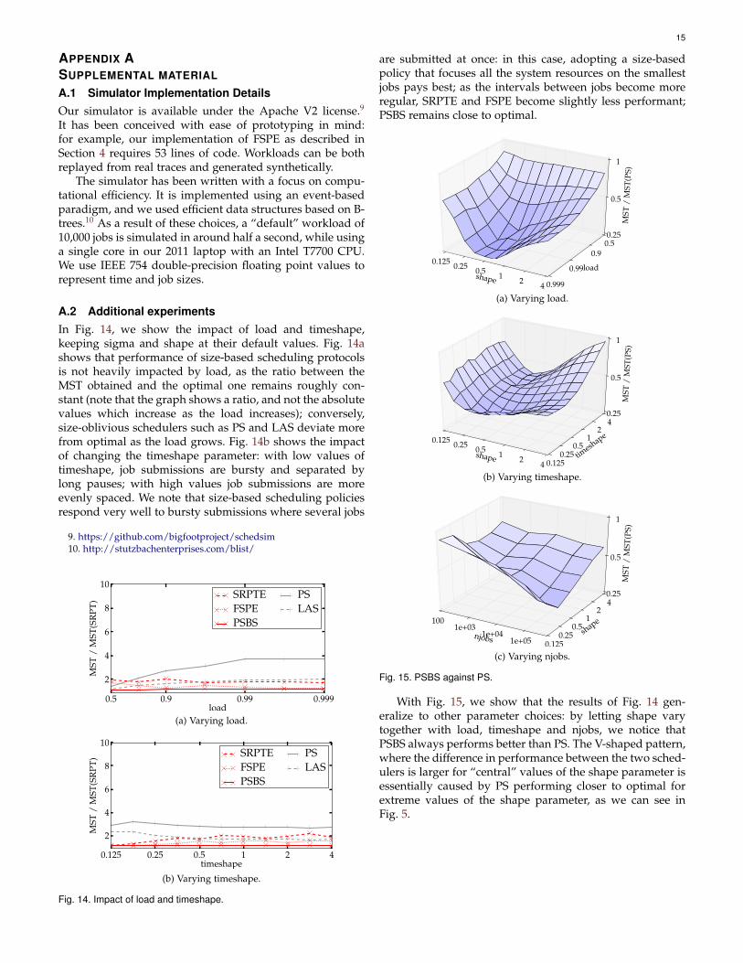
15

APPENDIX ASUPPLEMENTAL MATERIAL

A.1 Simulator Implementation DetailsOur simulator is available under the Apache V2 license.9

It has been conceived with ease of prototyping in mind:for example, our implementation of FSPE as described inSection 4 requires 53 lines of code. Workloads can be bothreplayed from real traces and generated synthetically.

The simulator has been written with a focus on compu-tational efficiency. It is implemented using an event-basedparadigm, and we used efficient data structures based on B-trees.10 As a result of these choices, a “default” workload of10,000 jobs is simulated in around half a second, while usinga single core in our 2011 laptop with an Intel T7700 CPU.We use IEEE 754 double-precision floating point values torepresent time and job sizes.

A.2 Additional experimentsIn Fig. 14, we show the impact of load and timeshape,keeping sigma and shape at their default values. Fig. 14ashows that performance of size-based scheduling protocolsis not heavily impacted by load, as the ratio between theMST obtained and the optimal one remains roughly con-stant (note that the graph shows a ratio, and not the absolutevalues which increase as the load increases); conversely,size-oblivious schedulers such as PS and LAS deviate morefrom optimal as the load grows. Fig. 14b shows the impactof changing the timeshape parameter: with low values oftimeshape, job submissions are bursty and separated bylong pauses; with high values job submissions are moreevenly spaced. We note that size-based scheduling policiesrespond very well to bursty submissions where several jobs

9. https://github.com/bigfootproject/schedsim10. http://stutzbachenterprises.com/blist/

0.5 0.9 0.99 0.999load

2

4

6

8

10

MST

/M

ST(S

RPT

) SRPTEFSPEPSBS

PSLAS

(a) Varying load.

0.125 0.25 0.5 1 2 4timeshape

2

4

6

8

10

MST

/M

ST(S

RPT

) SRPTEFSPEPSBS

PSLAS

(b) Varying timeshape.

Fig. 14. Impact of load and timeshape.

are submitted at once: in this case, adopting a size-basedpolicy that focuses all the system resources on the smallestjobs pays best; as the intervals between jobs become moreregular, SRPTE and FSPE become slightly less performant;PSBS remains close to optimal.

shape

0.125 0.25 0.5 12

4

load

0.50.9

0.99

0.999

MST

/M

ST(P

S)

0.25

0.5

1

(a) Varying load.

shape

0.125 0.25 0.5 12

4tim

eshape

0.1250.25

0.51

24

MST

/M

ST(P

S)

0.25

0.5

1

(b) Varying timeshape.

njobs

1001e+03

1e+041e+05

shape

0.1250.25

0.51

24

MST

/M

ST(P

S)

0.25

0.5

1

(c) Varying njobs.

Fig. 15. PSBS against PS.

With Fig. 15, we show that the results of Fig. 14 gen-eralize to other parameter choices: by letting shape varytogether with load, timeshape and njobs, we notice thatPSBS always performs better than PS. The V-shaped pattern,where the difference in performance between the two sched-ulers is larger for “central” values of the shape parameter isessentially caused by PS performing closer to optimal forextreme values of the shape parameter, as we can see inFig. 5.