#1...Projective Concepts & Projective Constructs in

Relativity and Quantum TheoryRoy Lisker

8 Liberty Street #306Middletown, CT 06457

rlisker@yahoo.comwww.fermentmagazine.org

May 12, 19991. Preface

Many fields of contemporary physics are modeled by non-Euclidean

geometry. [ 1,4,19,23,32 ] . 1 For most purposes, the 3 standard 2-D geometries

suffice : Euclidean, elliptic and hyperbolic. It is pointed out in this paper that

there are actually 9 such geometries, not counting variants arising from

particular restrictions . Each of these non-Euclidean geometries may in its turn

be embedded up to isomorphism into the real or complex projective planes,

RP2 and CP2 . [1, 11]

Geometric constructions derivable from the properties of lines, pencils

and points of pure projective geometry will be called “projective constructs”.

Many of the fundamental objects in modern physical theory are clearly

projective constructs. For example, the fiber bundle of light cones over

Minkowski Space is a projective construct.

For every projective construct there is a corresponding dual construct :

one switches the terms “line” and “point” , “intersection” and “collineation”,

etc., in the sentences that describe them.

A postulate for the physics of projective constructs is stated part way

through the paper:

1 Numbers in brackets refer to the Bibliography

#2...

Projective Postulate“ If the description of a natural

observation is a projective construct, then itsdual also exists in nature. “

The argument is mathematical, physical, and above all philosophical: the

ontology of projective entities is such that they must be cast in the form of dual

pairs to merit the existential predicate.

When the two principles of special relativity, the “Light Principle” (LP) , and

“Relativity Principle” (RP) are dualized, the resultant model, dual-Minkowski

space, bears a strong resemblance to the Hubble Field combined with the Big

Bang. It is possible that the expansion field of the cosmos may come directly

from the application of the projective postulate to special relativity.

The final section of this paper applies these ideas to quantum theory.

Arguments are presented to show that “uncertainty” is an fundamental

magnitude of nature. The fiber bundle of “uncertainty parabolas ” at each

point of time/moment space, J, forms the basis for wave-particle duality.

2. SummaryThe standard axioms for the projective plane in 2-dimensions exclude

parallel lines. However, the concept of parallel lines belongs to projective

geometry. This because this concept can be formulated entirely in terms of the

primitive notions of projective geometry: ‘point’ , ‘line’ , ‘intersection’,

‘colinearity’, ‘betweenness’ , etc. .

A concept stated in the language of projective geometry will be called

a “projective concept “ .

The existence of an entity P which can be described as a

projective concept is equivalent to the existence of its dual , Q, obtained by

switching the words ‘line’ and ‘point’, ‘intersection’ and ‘colineation’, in the

defining statement for P. For example: the concept dual to parallelism may be

#3...called seperalism 2 : points A and B in a given geometry are seperal if there

is no straight line on which they are collinear.

Projective constructs are models for projective concepts that can be

embedded in the projective plane, with redefinitions of the notions of “line”

and “point” based on the standard lines and points of the plane . This

redefinition must be done in such a manner that “intersection” retains its

customary meaning of ‘set intersection’ , and “colineation” retains its customary

meaning of common membership in a line .

The first part of this paper describes all of the standard non-Euclidean

geometries [12,...,17] , together with their seperal duals, as projective

constructs derived from projective concepts. The second part applies this range

of geometries to the representation spaces of modern theoretical physics. It is in

connection with this model that the projective postulate is stated and applied.

In the final part of this paper we propose a specific non-Euclidean

geometry , hyperbolic/dual-hyperbolic space , as the time/moment space of

quantum measurement. What we call the ‘knowable world’ lies in the region

below this parabolic fiber bundle and above the conic fiber bundle of special

relativity. Events not in this space are either impossible or unknowable or

both. 3ffffffffffff

3. Projective Concepts and Projective Constructs

2The unconventional spelling is deliberate; the word ‘separate’ is misspelt in standardEnglish.3There may however be reasons to assume their existence. See in particular Feynman [27]

#4...There exist projective geometries RPn ( CPn ) at all dimensions. The

situation in dimension 2 however has unique features which justify the

application of the term pure projective geometry (PPG) :

(1) The dualism of line and point is perfect only in PPG .

(2) The higher projective geometries are built out of combinations of the

properties of PPG .

(3) It is the ideal domain for embedding models of non-Euclidean

geometries.

The virtues of PPG have been noted by Alfred North Whitehead in his

thought provoking treatise on the subject, in which he calls it ‘ The science of

cross-classification ’ [ 5, pages 4,5]

There are standard models for PPG in both 2 and 3 dimensional

manifolds :

(1) PPG can be modeled on the (2-dimensional) surface , S, of the sphere

in 3-space, by identifying pairs of polar opposite points as “points”, and

defining as “lines” the great circles on S .

(2) An isomorphic model can be obtained through defining a “line” as a

2-dimensional linear sub-spaces, (planes) in Euclidean 3-space passing through

the origin, and a “point ” as the intersection sets of these planes, “Points”

become members of the pencil of lines passing through the origin.

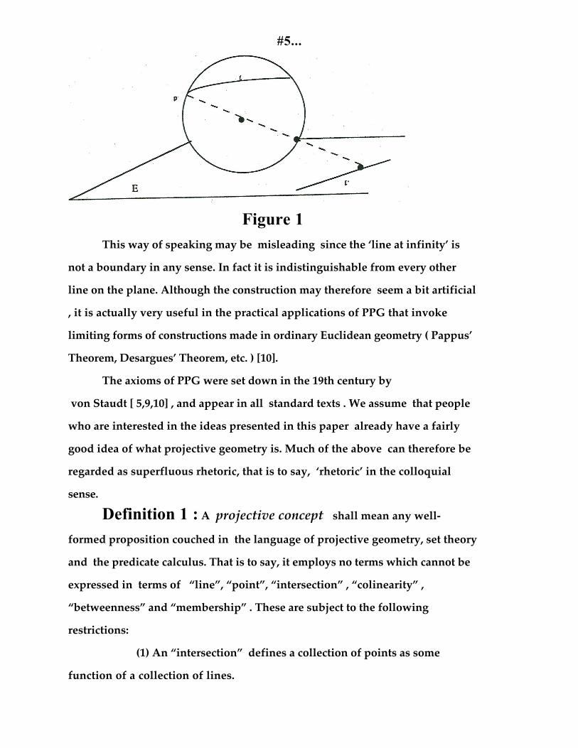
(3) The central projection of S onto a plane E2 tangent to its south pole

transfers the structure of PPG on S onto E2. One is obliged to adopt the

convention that the equator of S is sent out to a “line at infinity”

#5...

Figure 1This way of speaking may be misleading since the ‘line at infinity’ is

not a boundary in any sense. In fact it is indistinguishable from every other

line on the plane. Although the construction may therefore seem a bit artificial

, it is actually very useful in the practical applications of PPG that invoke

limiting forms of constructions made in ordinary Euclidean geometry ( Pappus’

Theorem, Desargues’ Theorem, etc. ) [10].

The axioms of PPG were set down in the 19th century by

von Staudt [ 5,9,10] , and appear in all standard texts . We assume that people

who are interested in the ideas presented in this paper already have a fairly

good idea of what projective geometry is. Much of the above can therefore be

regarded as superfluous rhetoric, that is to say, ‘rhetoric’ in the colloquial

sense.

Definition 1 : A projective concept shall mean any well-

formed proposition couched in the language of projective geometry, set theory

and the predicate calculus. That is to say, it employs no terms which cannot be

expressed in terms of “line”, “point”, “intersection” , “colinearity” ,

“betweenness” and “membership” . These are subject to the following

restrictions:

(1) An “intersection” defines a collection of points as some

function of a collection of lines.

#6...(2) A “colineation” defines a collection of lines as some function

of a collection of points.

A non-trivial example of a projectiveconcept:

Let L and M be two “lines” . Then the“intersection” of L and M will be a uniquepoint p, which is never a member of either L orM

Here is a model for this concept on the projective sphere S :

c

b

ad

L2

L1

p

L1 = a and bL2 = c and dInteresection = p

a

b

c

d

L1

L2

L1 = a and bL2 = c and d

Intersection = (i) Pole of (adb) if not c , in which case (ii) Pole of( cd ), if not a (iii) Then pole of (a,c)

K

G

H

#7...

Figure 2

In this geometry , a ‘line’ is defined as any non-polar pair of points , (

with their corresponding polar opposites ) on S . Two such ‘lines’ ‘intersect’ in

3 possible ways:

(1) If no 3 points are collinear, ( as defined by geodesics), and the

segments formed by geodesics through (a,b) and (c,d) intersect in a point p, then

p is defined as the “intersection” of the pairs (a,b) and (c,d)

(2) If d is collinear with the segment through (a,b) ,then we take the pole

of the geodesic, G, through (c,d) as the “intersection”, unless this coincides

with a ( or b ) . In that case we take the pole of the geodesic H through (a,b) as

the intersection. If this also coincides with c, then we draw a geodesic K

through c and b and take its pole as the intersection. By definition, this cannot

coincide with a (or b ) .

(3) If the geodesics through (a,b) and (c,d) coincide in a geodesic H, then

we take the poles of H as intersection .

In this way, every pair of lines, ( themselves defined as pairs of

#8... ( polar pairs ) of points), has a well-defined point associated with it which

does not belong to either of them and may be called the intersection point.

No “non-projective” ideas, such as “distance”, “neighborhood”, “finite” or

“infinite”, etc., were used in this construction. It therefore qualifies as a model

for a projective concept . It is not, however a projective construct in the sense

that we will be using it in this paper :

Definition 2 : A projective construct is defined to be a model for

some projective concept embedded in the pure projective plane. Specifically:Let the projective concept be designated as C . Let LC and PC stand for,

respectively, the line-element model , and the point-element model, of C .

Then:(1) LC and PC must themselves be projective concepts.

(2) LC and PC must be embeddable in PPG

(3) In these constructions the words “intersection” and “colineation” (

or their equivalents ) occurring in C must have the normal set-theoretic

meanings of intersection ( of lines considered as sets) and of membership

( of points within in lines considered as sets ) .

Thus, for a projective concept to be considered a projective construct, we

want geometry and standard set theory to come together. The above

construction is not, therefore , a projective construct.

Clearly anything that can be “drawn” in PPG , using standard line and

point concepts defined by its axioms , is a projective construct. Thus, the

notions of “triangle” , “4th harmonic point” , “simple closed curve”, even

“convex figure” , are projective concepts for which there exist projective

constructs in PPG without alteration of the basic point and line elements. ( One

must enrich PPG sufficiently to allow for the definition of Jordan curves, but

this presents no difficulty ).

#9...An example of a projective concept for which there can be no projective

construct ( by our definition) is a self-intersecting line . Such a object implies

two contrary uses of the word “intersection”:

(1) The line L “intersects “ with itself in the sense of set theory. This

intersection is just the entire line, L .

(2) The geometric “intersection” in the sense of the self-intersecting

boundary of a curve . For a projective construct the two meanings must

coincide. The only possible model for such a linear element , which is also a

projective construct, is that in which every point p is also a line L . One might

call this the “trivial geometry”.

Figure 3

Here is the point of the exercise: Any statement C in the form of a

projective concept automatically generates its dual form , Y , which is also a

projective concept. If there is a model for C which qualifies as a projective

construct, then there is automatically a model for Y which qualifies as a

projective construct. If C occurs in some physical theory and is correlated with

an observable in nature, then there must be another observable in nature

which correlates with Y ; otherwise C has been inconsistently defined, or the

#10...projective space used to represent this aspect of the natural world is self-

contradictory or inadequate . If we haven’t found Y yet, we must keep looking

for it. Otherwise we must abandon C.

As we will show, all of the standard, as well as some unconventional,

non-Euclidean geometries can be modeled in PPG as projective constructs of

projective concepts.

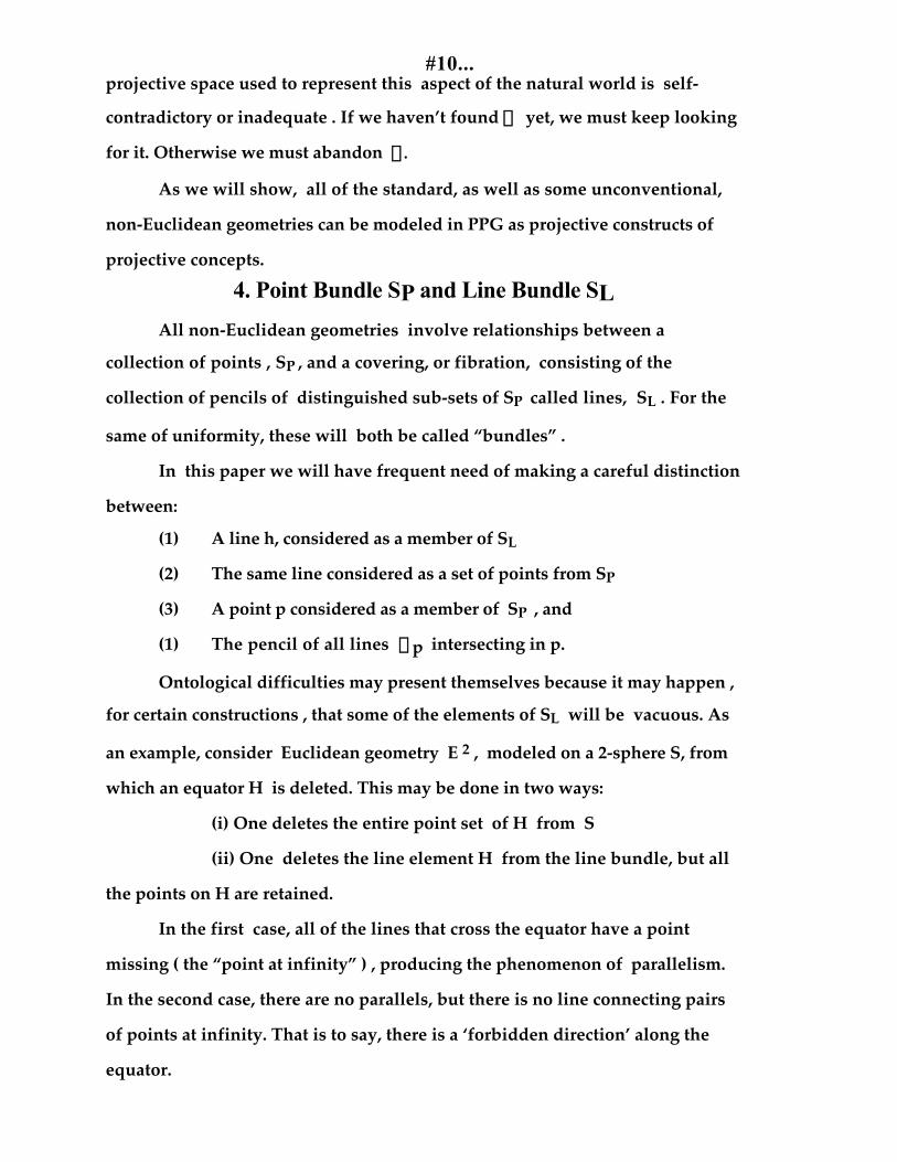
4. Point Bundle SP and Line Bundle SL

All non-Euclidean geometries involve relationships between a

collection of points , SP , and a covering, or fibration, consisting of the

collection of pencils of distinguished sub-sets of SP called lines, SL . For the

same of uniformity, these will both be called “bundles” .

In this paper we will have frequent need of making a careful distinction

between:

(1) A line h, considered as a member of SL

(2) The same line considered as a set of points from SP

(3) A point p considered as a member of SP , and

(1) The pencil of all lines Pp intersecting in p.

Ontological difficulties may present themselves because it may happen ,

for certain constructions , that some of the elements of SL will be vacuous. As

an example, consider Euclidean geometry E 2 , modeled on a 2-sphere S, from

which an equator H is deleted. This may be done in two ways:

(i) One deletes the entire point set of H from S

(ii) One deletes the line element H from the line bundle, but all

the points on H are retained.

In the first case, all of the lines that cross the equator have a point

missing ( the “point at infinity” ) , producing the phenomenon of parallelism.

In the second case, there are no parallels, but there is no line connecting pairs

of points at infinity. That is to say, there is a ‘forbidden direction’ along the

equator.

#11...What are the corresponding procedures for the construction of E2

models for dual- Euclidean geometry E*2 ?

(1) One deletes the entire pencil of lines emanating from the

North ( South) pole ; or

(2) All these lines are retained ; one merely excises the North

(South) pole from the geometry. One can then ask if the North/South pole

“exists” in this geometry. Is it perhaps a “void point”, like the “void sets” of

conventional set theory? Dualism, indeed, seems to suggests that the concept of

the “void point” merits a place in Projective Geometry.

The interdependence of point- and line bundles implies two distinct, yet

co-extensive, ways of defining lines and points.

In the models we will construct for the non-Euclidean geometries, a line

l will be defined as either:

(1) The set of points belonging to l ; or

(2) A particular member of SL collinear with a certain pair of points

A point p , likewise, is either:

(3) A member of SP ; or

(4) The intersection of two elements of SL .

That this is more than mere quibbling can be seen from the following

definition:

Definition 3 : Let CL and CP be , respectively, subsets of SL

and SP , defined as projective concepts, for which there are projective

constructs in PPG.

Let Cint be the set of all intersections of pairs of elements of CL ; and

Ccol the collection of pre-images of the mapping of the elements of CP into

their ( corresponding ) lines in CL .( As observed above, these may sometimes

be vacuous.)

Then any combination of the form ( CL , CP ) , ( CL , Cint ) ,

#12...( Ccol , CP ), (Ccol , Cint ) , will be said to define a non-Euclidean

geometry , or simply a geometry , in PPG .

The intent of this definition is best illustrated by an example: let C be a

closed convex curve in the upper half-sphere S1/2+ . ( This implies the

construction of its polar opposite C* in the lower half sphere S1/2- ) . Remove

S = interior of ( C,C*) from S, leaving us with a connected region D = S/ S on

the sphere . In setting up a geometry over D , one can choose for the elements

of the line-space:

(1) The great circles that remain entirely in D , or DL

(2) These, and in addition, all the truncated segments of great circles

which touch on the boundary of G . This is D col .

These geometries are rather different.

(1) The geometry defined by (DL , DP ) has many seperal point

pairs, namely those that are not collinear with great circles entirely in D .

There are no parallels in this geometry, which is ‘dual-hyperbolic’ in our

sense.

(2) The geometry defined by (Dcol , DP ) has no seperal pairs;

however, many ‘lines’ will not intersect. It is therefore ordinary hyperbolic

geometry, indeed a Poincaré -Beltrami model [12,…17]

5. Classification and Construction of

Non-Euclidean Geometries

The 3 traditional non-Euclidean geometries are distinguished through

conditions on parallelism : one parallel (Euclidean) , no parallels

(Riemannian) , and many parallels (Lobatchevskiian) , to a line L through a

point p not on L . For convenience we will call these ‘flat’, ‘elliptic’ and

‘hyperbolic’ geometries.

Projective constructs could be used to model a far greater variety of

non-Euclidean geometries. ( For example: define a “line” as any pair of lines in

the projective plane, and a “point” as any 4-point set, no 3 of which are

#13...collinear. In this geometry, two lines define at most one point, and at most 3

lines pass through a point. )

Dualizing the 3 traditional geometries creates 3 geometries based on

the properties of seperalism. Furthermore, there exist geometries which

combine conditions on line parallelism and point seperalism in various ways.

The complete description of the projective concept of parallelism in PPG

therefore involves 9 distinct geometries.

Definition 4 : Two points in a geometric space are called seperal if

there exists no line on which both of them are incident.

Definition 5(a): A geometry will be said to be dual-flat , or have the

unique seperal property if, given a point p and a line L on which p is not

incident , there exists one and only one point q on L which, with p, forms a

seperal pair.

(b): A geometry will be said to be dual-hyperbolic , or

have the many seperal property if, given a point p and a line L on which p is

not incident , there exist many points on L which form a seperal pair with p.

(C): A geometry will be said to be dual-elliptic , or

have the no seperal property if any two points can be connected by at least

one line.

(6) Representations of Parallelism in PPG :

The non-Euclidean geometries

1. Elliptic/Dual-Elliptic … No parallels ; No seperals(Riemannian)

2. Flat/Dual-Elliptic … Unique parallel; No seperals(Euclidean)

3. Hyperbolic/Dual-Elliptic … Many parallels; Noseperals (Lobatchevskiian)

4. Elliptic/Dual-Flat … No parallels; Unique seperal

#14...(Dual Euclidean )

5. Flat/Dual-Flat … Unique parallel; Unique seperal( Two Dimensional Classical Space-Time )

6. Hyperbolic/Dual-Flat … Many parallels; Uniqueseperal

(Dual Minkowski )7. Elliptic/Dual-Hyperbolic … No parallels; Many

seperals(Dual Lobatchevskiian)

8. Flat/Dual-Hyperbolic … Unique parallel; Manyseperals(Minkowskian )

9. Hyperbolic/Dual-Hyperbolic ..Many parallels;Many seperals(Quantum Time/Moment Space)

These geometries cover the combinations of parallel and seperal conditions

. Most of them have found applications as representation spaces for models of

phenomena in contemporary physical theories. One might of course also look

at other species of Non-Euclid/Hilbert geometries for the modeling of

phenomena : Non-Desarguen spaces , p-adic arithmetics , ( which are Non-

Archimedean ) , and so on. For the present esoterica of interest mainly to

mathematicians, they may well become useful in the future [10] . We now

examine each geometry in turn:

(a) Elliptic/ Dual-Flat Geometries Euclidean plane geometry is modeled directly in the projective plane

by a familiar construction: Represent PPG as the geometry of great circles with

identification of polar pairs on a spherical surface , S. Remove the equator H

from the line bundle, and the equatorial points from the point bundle .

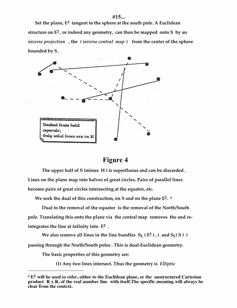
#15...Set the plane, E2 tangent to the sphere at the south pole. A Euclidean

structure on E2 , or indeed any geometry, can then be mapped onto S by an

inverse projection , the ( inverse central map ) from the center of the sphere

bounded by S .

Figure 4The upper half of S (minus H ) is superfluous and can be discarded .

Lines on the plane map into halves of great circles. Pairs of parallel lines

become pairs of great circles intersecting at the equator, etc.

We seek the dual of this construction, on S and on the plane E2. 4

Dual to the removal of the equator is the removal of the North/South

pole. Translating this onto the plane via the central map removes the and re-

integrates the line at infinity into E2 .

We also remove all lines in the line bundles SL ( E2 ) , ( and SL( S ) )

passing through the North/South poles . This is dual-Euclidean geometry.

The basic properties of this geometry are:

(1) Any two lines intersect. Thus the geometry is Elliptic 4 E2 will be used to refer, either to the Euclidean plane, or the unstructured Cartesianproduct R x R, of the real number line with itself.The specific meaning will always beclear from the context.

#16...(2) Two points p and q on a longitude on S ,( or line passing

through the excised origin on E2 ) , will have no line through them.

(3) If H is a line not passing through the origin, and p a point not

on H, then there is only one point q on H ( recall that the line at infinity has

been restored ) which is seperal to p. Hence the geometry is Dual Flat

One can also represent elliptic/dual-flat geometry by a model which

incorporates the line at infinity within the finite part of the plane. Remove the

origin on E2 , and parametrize locations by polar coordinates ( r , q ) , r ≠ 0 .

Define the line space as the set of curves:r = Aexp(bq )A > 0 b ≠ 0 - • < q < +•

In this geometry, two points with different values of q but the same value

of r will be seperals. We will have occasion to return to this model in our

discussion of Dual Relativity.

(b) Flat/Dual Flat GeometriesThere are two simple ways of modeling flat/dual-flat geometry as a

projective construct. Such a geometry will have both the “unique parallel”

and the “unique seperal” properties. On S:

I. (i) Remove an equator from the line bundle.

(ii) Remove the points on the equator from the point bundle.

(iii) Remove the poles of this equator

(iv) Remove the line pencil that connects the poles,

The symmetry of this procedure insures a self-dual geometry

II. (i) Remove an equator from the line bundle , and the equatorial points

from the point bundle .

(ii) Remove an entire pencil of lines between some polar pair on

the equator itself .

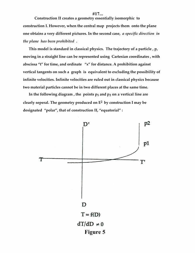
#17...Construction II creates a geometry essentially isomorphic to

construction I. However, when the central map projects them onto the plane

one obtains a very different pictures. In the second case, a specific direction in

the plane has been prohibited .

This model is standard in classical physics. The trajectory of a particle , p,

moving in a straight line can be represented using Cartesian coordinates , with

abscissa “t” for time, and ordinate “x” for distance. A prohibition against

vertical tangents on such a graph is equivalent to excluding the possibility of

infinite velocities. Infinite velocities are ruled out in classical physics because

two material particles cannot be in two different places at the same time.

In the following diagram , the points p1 and p2 on a vertical line are

clearly seperal. The geometry produced on E2 by construction I may be

designated “polar”, that of construction II, “equatorial” :

Figure 5

#18...

( c ) Hyperbolic and Dual-HyperbolicGeometries

Constructions for the hyperbolic geometries differ from those of flat

and elliptic geometries, in that the mere removal of lines, line pencils, or

points, from either the line bundle or the point bundle is inadequate to the

task of embedding them in PPG . Poincare-Beltrami models and others require

the introduction of closed convex curves , non-self-intersecting curves, ( thus

entirely in S1/2+ ( S1/2- ) ) , for which “ interior” and “exterior” can be defined.

It is here that the distinction between a line defined as an element of a

collection of truncated lines , or as a certain kind of subset of the point bundle

, becomes meaningful.

Fix a line, H , as equator, with corresponding North/South pole Y =

(N,S) . We assume that the notion of a simple , connected, non-self-intersecting

curve S = ( C, C* ) on S is clear. The interior of S is defined as that region

including Y .

S is convex if:

(1 ) It does not intersect H

(2) Let p and q be interior points of S . Then one of the two segments of the

line ( great circle ) between p and q does not intersect S .

Let D be the exterior of S , G its interior . D is certainly connected. Also,

since S does not intersect H , D contains at least one great circle. G does not

contain any. Therefore we will call D the “exterior geometry” and G the

“interior geometry” .

Theorem:(1) There is a geometry inside G , definable via a projective construct,

which is hyperbolic/dual- elliptic , and a dual geometry inside D which is

elliptic/dual-hyperbolic.

#19... (2) If S is a polar pair of circles , and the radius of this circle is 1/4 of

the arc of a great circle, then the interior geometry , and the exterior geometry

are exactly dual.

Proof:(1) Let a, b, c and d be any 4 points on S , arranged sequentially in

either clockwise or counter-clockwise order. Connect a and d by a segment s1

cutting across G . Connect b and c by a similar segment s2 .

Figure 6The Axioms of Order of Projective Geometry guarantee that s1 and s2

will not intersect. We can then consider the two segments as “parallels”. If e is

on the arc between d and c ( not containing a or b ) , then the line s3 = ( ae )

intersects the line s1 = (ad) only on the boundary. This allows us to treat S

as the Absolute in the Poincare-Beltrami construction for a hyperbolic

geometry. Since C is convex, any two points in G can be connected by a “line”.

This geometry is therefore also dual-elliptic.

#20...

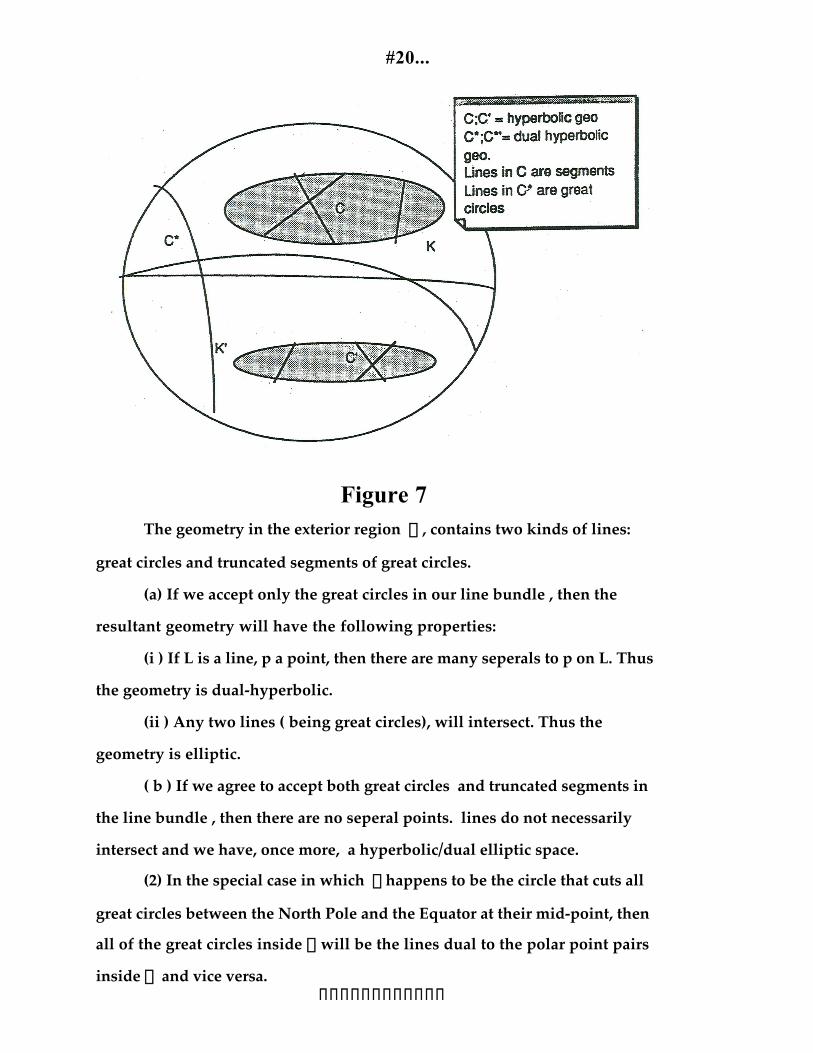
Figure 7The geometry in the exterior region D , contains two kinds of lines:

great circles and truncated segments of great circles.

(a) If we accept only the great circles in our line bundle , then the

resultant geometry will have the following properties:

(i ) If L is a line, p a point, then there are many seperals to p on L. Thus

the geometry is dual-hyperbolic.

(ii ) Any two lines ( being great circles), will intersect. Thus the

geometry is elliptic.

( b ) If we agree to accept both great circles and truncated segments in

the line bundle , then there are no seperal points. lines do not necessarily

intersect and we have, once more, a hyperbolic/dual elliptic space.

(2) In the special case in which S happens to be the circle that cuts all

great circles between the North Pole and the Equator at their mid-point, then

all of the great circles inside D will be the lines dual to the polar point pairs

inside G and vice versa.ffffffffffff

#21...

(d) Elliptic/Dual Hyperbolic GeometryProject the region D onto E2 by the central map . The resultant planar

region will be Euclidean space with a hole at the origin. Adjoining the line at

infinity, ( the projection of the equator ) , and treating as line elements only

those complete lines in E2 which are not truncated by the hole at the center,

one creates a model for elliptic/dual-hyperbolic geometry: no parallels, many

seperals: any two points collinear to a line passing through the hole will be

seperal. Topologically D is a torus.

(e) Self-Dual Hyperbolic GeometrySelf -dual hyperbolic geometry can be modeled through simple

modifications of preceding models : Let G be, as before, stand for the interior

of S = ( C,C* ) .

Draw another convex loop, D , ( with corresponding polar

loop D’ ) inside S and containing the North Pole Y . The space between C

and D is an annulus, A . It is naturally self-dual: two lines ( defined as

segments of great circles truncated by both C and D ) intersect in at most one

point. Pairs of points are collinear to at most one line. Every point p in A

supports a “cone” of lines, a truncation of the pencil of

( truncated! ) lines holding p. One must, of course , remove all lines , (such as k

= (be) in the figure below) , from the line bundle on S passing through the

region enclosed by D .

#22...

Figure 8

(f) Pseudo Flat and Dual Pseudo FlatGeometries

The two remaining geometries, VI and VIII are familiar as

representation spaces for theoretical physics. The appropriate projective

constructions on S ( or PPG ) not so intuitive as the previous ones. VIII is also

called pseudo-Euclidean geometry , an expression which does not refer to its

parallel/seperal structure but to the indefiniteness of its Riemannian metric. In

our terminology, pseudo-Euclidean geometry is flat/dual-hyperbolic.

On S:

Let g be some arbitrarily chosen segment of the equator H. less than p

in length so as not to intersect its polar equivalent g’. ( This is not really a

length restriction. It merely states that g is a piece and not the whole, of the

equator , which is a proper projective concept. )

Remove from the line bundle all lines passing through the segments g

and g’ . Then remove H from the line bundle, and the points on H from the

point space .

#23...This is pseudo-Euclidean geometry . When transferred to E2 , one

obtains a Minkowski space. There is a “prohibited cone” at each point p ,

derived from the lines passing between the poles and the segment g ; and a

“permissible cone” , ( with central angle q = p - g ) , of the remaining lines

through p . Following standard practice, the axis of the permissible cone is

aligned with the vertical direction of time.

There is a slight difference in the models for Special Relativity

depending on whether

(i) The segment g is open ended; or

(ii) g is closed

If g is a closed set, then the “light path ” is in the prohibited cone, and

cannot be attained on the permissible cone. This is the relativistic universe of

matter alone. If g is an open set , then it may be possible to travel at velocity

c, but not beyond. This is the geometry of matter plus radiation. Special

Relativity indeed, distinguishes 3 distinct regions: time-like, space-like, and

that upon the light cone itself.

This model can be extended. In fact, one is free to remove several

segments g1 , g2 ,... , gn . from the equatorial line , H, together with the

truncated pencils of all lines passing through them. The resulting space is still

flat/dual-hyperbolic, yet now contains several limiting velocities , with

“windows” of permissibility interspersed between them. Thus, one might be

able to travel with a velocity less than c1 ; greater than c2 but less than c3 ;

greater than c2n but less than c2n+1 ; and so on.

#24...

Figure 9One is speaking projectively of course, not in terms of the Riemannian

metric for proper time, which might become rather complicated. However, for a

simple model involving two limiting velocities u = c2n< v = c2n+1 , it is not

difficult to construct a Riemannian metric that expresses the idea that velocities

are constrained to be greater than u but less than v This metric takes the form:

ds2 = (dx - udt)(vdt - dx) = -dx2 + dxdt(u + v) - uvdt2

One might conjecture from this that the 4 fundamental forces of nature

could each possess a distinct velocity of propagation. The speed of the

graviton might exceed that of the quantum! Perhaps it is possible to travel

faster than gravity, but not at any speed between light and gravity, and so

forth . Since this idea is consistently represented by a projective construct, it

should not be dismissed without investigation.

(g) Dual-Minkowski Space Our next model is that of dual - pseudo-Euclidean geometry. The

North/South polar pair, Y , is dual to the equator, H. Dual to the segment ( g,

g’ ) on H is the pair of sectors , K=(J,J*) , between great circles meeting in

Y and intersecting the equator with a separation g .

#25...

Therefore:(i) Remove all the points in J and J’ from the point bundle .

Remove all ( north-south) longitudes composed of these points from the line

bundle . The “lines” of this geometry are the truncations of all remaining

great circles on S.

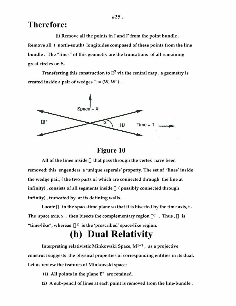
Transferring this construction to E2 via the central map , a geometry is

created inside a pair of wedges F = (W, W’ ) .

Figure 10All of the lines inside F that pass through the vertex have been

removed: this engenders a ‘unique seperals’ property. The set of ‘lines’ inside

the wedge pair, ( the two parts of which are connected through the line at

infinity) , consists of all segments inside F ( possibly connected through

infinity) , truncated by at its defining walls.

Locate F in the space-time plane so that it is bisected by the time axis, t .

The space axis, x , then bisects the complementary region GC . Thus , F is

“time-like”, whereas FC is the ‘proscribed’ space-like region.

(h) Dual RelativityInterpreting relativistic Minkowski Space, M1+1 , as a projective

construct suggests the physical properties of corresponding entities in its dual.

Let us review the features of Minkowski space:

(1) All points in the plane E2 are retained.

(2) A sub-pencil of lines at each point is removed from the line-bundle .

#26...(3) The remaining sub-pencils at each point subtend identical angles and

have parallel boundaries.

(4) The line at infinity is also excised , allowing for a unique parallels

geometry with corresponding (pseudo) Euclidean metric.

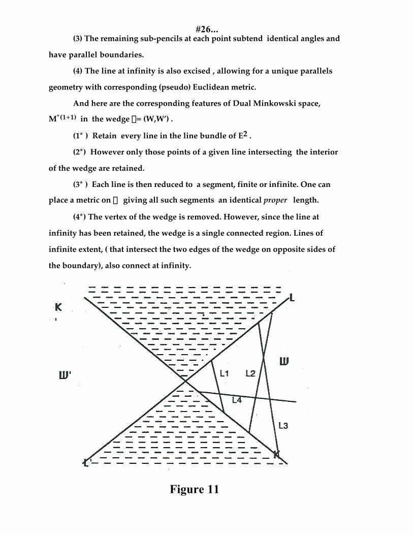
And here are the corresponding features of Dual Minkowski space,

M*(1+1) in the wedge G= (W,W’) .

(1* ) Retain every line in the line bundle of E2 .

(2*) However only those points of a given line intersecting the interior

of the wedge are retained.

(3* ) Each line is then reduced to a segment, finite or infinite. One can

place a metric on F giving all such segments an identical proper length.

(4*) The vertex of the wedge is removed. However, since the line at

infinity has been retained, the wedge is a single connected region. Lines of

infinite extent, ( that intersect the two edges of the wedge on opposite sides of

the boundary), also connect at infinity.

Figure 11

#27...This is the model for dual Special Relativity . A possible physical

interpretation of its geometric properties is :

(i) Although the vertex of the wedge is removed from space-time, since

the line at infinity has been restored the wedge is a simply connected convex

region.

(ii) One might interpret the vertex as the moment of the Great Explosion.

(iii ) The trajectories of material bodies cannot pass through the origin.

An observer located there can perceive nothing going away nor moving

towards himself.

Equivalently, one might say that the straight lines emanating from the

origin are purely temporal trajectories emerging from the Great Explosion.

Observers on straight line trajectories passing through the origin cannot

observe the passage of time, even as a person in a spatial location in

Minkowski space has no absolute way of knowing if he is traveling or

standing still. ( The dual Relativity Principle . )

(iv ) There do not exist space-time locations for whichx t > gg = tan(a)a = vertex angle

(v) Dual to spatio-temporal location is the notion of a spatio-temporal

trajectory. Trajectories inside the wedge can be interpreted as photon paths

terminating at the walls of the wedge .

(vi ) The points at which they terminate can be called staticons .

Staticons move along the boundary at a velocity v determined by the Hubble

expansion acceleration, g = v/ T .

(vii) As long as v < c , the speed of light , quanta will overtake the

Hubble expansion and must therefore merge into staticons . Under the

hypothesis that the Hubble velocity can never exceed light, all radiation

becomes absorbed at the boundary by a staticon, ( which may be equivalent to

#28...the Hawking/Penrose interpretation of a Black Hole as a boundary point of

cosmic space-time.) All radiation therefore begin and end in a staticon.

(viii) One may also state a dual Light Principle for dual-Minkowski

space: The distance from any point in the interior to any staticon is g.

g is the proper distance which a quantum must travel before it reaches the

boundary of the Hubble expansion .

In the figure below Space-Time is the interior of the pair of wedges.

The forward direction of time is off to the right, the forward direction of space

towards the top of the page. Trajectories L1 and L2 have been drawn

connecting the bounding walls. They have length “g” . The line connecting U

with V has length less than g.

Figure 12The similarities between this geometry and that of the Hubble

expansion field are evident. Notice also how it contains a combination of both

Big Bang and Steady-State evolution: some kind of “dual matter” is “born” at

a staticon and “vanishes” at another, depending only on its velocity; this is the

#29...Steady-State model. However, as the universe expands, new particles require

longer periods of time to disintegrate.

Special Relativity, plus the dualization of Minkowski space, may turn

out to be enough to derive and describe the Hubble expansion field.

Further support to this hypothesis comes from this via a parametrization which

“extends” the wedge over the entire plane. Finite line segments are mapped

onto by infinite exponential spirals radiating outwards from a common

origin.Their equations, in polar coordinates r, q , are :

r = eH(q +m ) 0 £ m £ 2p

Figure 13 The points A and B lie on different world-lines emerging from the

Great Explosion. The “ proper length” between them is the rotation angle ( or

tangent thereof), between their two world-lines. The radius vector, r , may be

identified with ‘time’, while the arc length of the unique exponential spiral

#30...

P = eL(q +a ) between them may be identified with ‘distance’, (

appropriately normalized). Observe that no such spiral can be drawn when A

and B are equidistant from the origin.

The physical interpretation of this is the following: two events

occurring at an identical ‘world time’ from the Great Explosion, cannot be

connected by a space-time geodesic and are causally independent.

6. The Projective Postulate Dualization of Minkowski space produces a dual-geometry. Physical

entities modeled in the former representation space go over into entities in

latter , which ought to turn up as observables in nature. The connection

between Special Relativity and the Hubble expansion is suggestive, and

appears to derive from a physical principle which we have named the

Projective Postulate. Note its similarities to both the complementarity of Niels

Bohr and Dirac’s conception of anti-matter and bra-ket formalism. [ 24 -33] :

Projective Postulate“ If the description of a natural

observation is a projective construct, then itsdual also exists in nature. “

To say that an observable M is “projective” implies that, in the very

act of its formulation, there is a back-reconstruction of a projective space P

in which it is embedded . If its dual did not automatically exist by virtue of a

co-dependent relationship, then M would not be truly projective. “Projective”

concepts, by their very nature, arise only in dual pairs, in the same way that

‘foreground/ background’ , ‘inside/ outside’, ‘more/ less’ , etc. , cannot be

defined independently.

Examples of Projective Constructs and theirDuals.

#31...The list of projective constructs in modern physics, with their

projective duals, includes :

(i)Construct: The path of the quantum, considered as particle.

Dual Construct : The pencil of light rays about any

unconstrained source of radiation, a wave phenomenon.

(ii )Construct : The limiting velocity of the speed of light

Dual Construct : The Hubble expansion field.

(iii) :Construct : The light cone as point space ( particles )

Dual Construct :The light cone as line space (waves )

(iv.): Construct/Dual Construct : Position Space/ Momentum Space

dualism in the Operator/Hilbert Space treatment of quantum theory

(v.):Self- Dual Construct : Uncertainty as quantity in Quantum

Theory

(See section 10 )

Commentary :(i) The metric geometry of Minkowski space allows one to treat the

quantum world-line as a point: the proper time distance of any two events on

its trajectory is 0. This is suggestive of the way in which the projective plane

is constructed in 3-space, through the identification of each line through the

origin of E3 with a point on the surface of the unit sphere. A light cone is

simply a plane of these “points” in 4-space intersecting the spherical surface

#32...in a great hyper-circle, which may be treated as a wave packet emanating

outwards in all directions from a light- source .

(ii) See section 5h.

(iii) A horizontal cross-section of the cone is a radiative light-pencil in

3-space. The ellipsoids arising from intersections of the light cone with

horizontal hyper-planes function as ‘hyper-lines’ in a 3-dimensional

projective geometry. This point of view is developed in Penrose’s Twistor

Geometry.

(iv) It is self-evident that the “phase space” of Quantum Theory is quite

different from the “phase space” of Statistical Mechanics or Hamiltonian

Dynamics. In the operator calculus of Quantum Theory one is free to describe

phenomena in a “momentum formalism ” or a “position formalism ”, these

descriptions being mediated by the Fourier Transform. In effect, the operator

calculus of Quantum Theory acts over a projective space, with its co-dependent

point and line bundles .

(v) The projective character of quantum uncertainty is discussed in the

next section.ffffffffffff

(8) Physical Applications

This completes the construction and classification of all Euclidean

geometries derived from the negations , duals and dual-negations of the

parallel postulate. Many of them already fulfill roles as representation

spaces for modeling the phenomena of modern physical theory:

(1) Elliptic/Dual-Elliptic : The basic representation space for geology

and astronomy. Spherical trigonometry

#33...(2) Flat/Dual-Elliptic : The stationary atemporal reference frame in the

absence of gravitation. Euclidean geometry

(3) Hyperbolic/Dual-Elliptic: In Einstein’s famous example of the

“warping” of Euclidean geometry on the plane of a uniformly rotating disk,

the metric geometry is hyperbolic. Gravitational fields create local hyperbolic

geometries. Hyperbolic geometry also occurs frequently in Optics.

(5) Flat/ Dual-Flat : The self-dual phase space of Quantum Theory

(6) , (7) . No present applications, although a suggested application for

(6) is given in this paper.

(8 ) Flat/Dual Hyperbolic : Special Relativity

(9) Hyperbolic/ Dual Hyperbolic : We will relate this to the geometry of

quantum uncertainty.

It would come as no surprise the author if it turns out that all of the

non-Euclidean geometries are required for the modeling of the physical

universe. The evidence seems to show that the universe is projective rather

than metric in its fundamental geometric structure.

(9) Quantum Theory and Projective Geometry

In classical physics matter is a scalar magnitude, functioning more or

less as a multiplicative parameter. In the statement of Newton’s law of

universal gravitation, the masses of attracting objects enter in the form of a

simple product, linear in each . In the expressions for energy and momentum,

mass is only a constant of proportionality.

Treating matter as a scalar means that , unlike space, ( and in this century,

time ) , matter has no intrinsic geometry . This despite the fact that , as was

noted by Aristotle , material objects, ( unlike temperatures, pressures and

various other magnitudes ) , always present themselves to our senses in the

form of 3-dimensional shapes . However, the apparent solidity of matter,

challenged already by Democritus, evaporates in elementary particle theory

#34...into a collection of force fields and binding connections between mathematical

points.

Not being “geometrical”, classical matter cannot be treated as a

projective construct: substance has no dual correlative. Yet characteristics dual

to those of matter were discovered in the behavior of radiation. These became

incorporated in the idea of a field, described mathematically by James

Maxwell. Fields, ( propagated across regions of the universe ) , are duals of

particles, ( best seen as compact systems in isolation . ) Before the development

of quantum theory , no connections were believed to pertain between the

“radiating” field and the “punctual” particle.

Quantum Theory has connected space , time , matter and energy

within a single self-dual flat geometry . Even as the localization ambiguities

of light become incorporated in projective constructs in Special Relativity , so

the localization ambiguities of matter are expressed through projective

constructs in Quantum Theory. At the same time, the hyperbolic or Riemannian

geometries appropriate to Special and General Relativity, and the dual

position/momentum picture of Quantum Theory, are not compatible .

Observe that General Relativity does ascribe a kind of geometric

structure to matter, via Mach’s Principle for Inertia, and the Curvature Tensor

interpretation of gravitation. In this instance “mass” functions as a kind of

connection in the fiber above space-time as base. There is clearly a world of

difference between the Space/Time/Matter geometry of Quantum Theory, and

the Space/Time/Matter geometry of General Relativity.

It comes as no surprise that it turns out to be so difficult to combine

these theories, as is attempted for example in Quantum Gravity. Not only must

there be a way of casting all the laws of nature into a co-variant form, but

every Observable implies the existence of a dual Observable. In line with the

Projective Postulate, it would appear, in particular , that any successful

#35...resolution of the conflict between Relativity and Quantum Theory requires

the existence of dual-relativistic Observables in a dual-Minkowski space.fffffffffffffffffffffff

(10 ) The Self-Dual Hyperbolic Geometry of Quantum

Uncertainty

Let an object O, of mass m , be under observation, ( such as an electron,

whose mass is known in advance.) We wish to embed the measurement process

on O in a 2-dimensional uncertainty space , J . The two dimensions of J are

“time”, t and “moment” y = mx , where x is position, ( 1-dimensional for

convenience ) . A point in J will plot our knowledge of the state of O. We

will assume, without loss of generality , that O’s state has been measured and

that, within the latitude afforded by the Uncertainty Principle, has been shown

to be “at rest” and “ at the origin” of the frame of the investigator.

One way of expressing this is by stating: We are certain that O lies

something within a rectangular box , B , in J , with vertices ( 0, 0 ) ; ( 0,y) ;

( t,0 ) ; and ( t , y ) :

Figure 14The actual values of t and y are given by the assumption that the trade-

off in position and momentum errors must be greater than or equal to h/4p . If

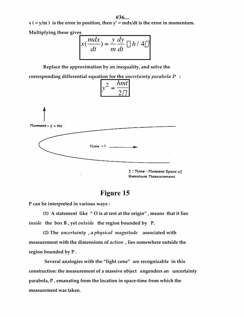
#36...x ( = y/m ) is the error in position, then y’ = mdx/dt is the error in momentum.

Multiplying these gives

x(mdxdt

) =ym

dydt

ª h / 4p

Replace the approximation by an inequality, and solve the

corresponding differential equation for the uncertainty parabola P :

y2 =hmt2p

Figure 15P can be interpreted in various ways :

(1) A statement like “ O is at rest at the origin” , means that it lies

inside the box B , yet outside the region bounded by P.

(2) The uncertainty , a physical magnitude associated with

measurement with the dimensions of action , lies somewhere outside the

region bounded by P .

Several analogies with the “light cone” are recognizable in this

construction: the measurement of a massive object engenders an uncertainty

parabola, P , emanating from the location in space-time from which the

measurement was taken.

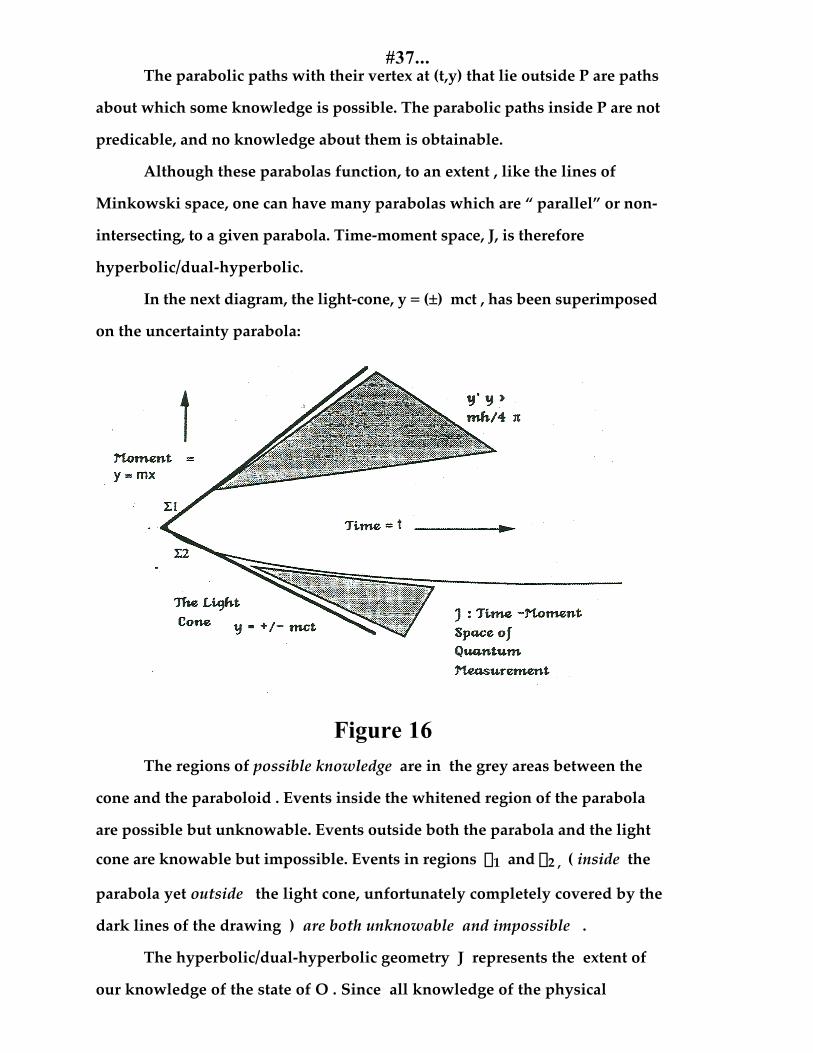
#37...The parabolic paths with their vertex at (t,y) that lie outside P are paths

about which some knowledge is possible. The parabolic paths inside P are not

predicable, and no knowledge about them is obtainable.

Although these parabolas function, to an extent , like the lines of

Minkowski space, one can have many parabolas which are “ parallel” or non-

intersecting, to a given parabola. Time-moment space, J, is therefore

hyperbolic/dual-hyperbolic.

In the next diagram, the light-cone, y = (±) mct , has been superimposed

on the uncertainty parabola:

Figure 16The regions of possible knowledge are in the grey areas between the

cone and the paraboloid . Events inside the whitened region of the parabola

are possible but unknowable. Events outside both the parabola and the light

cone are knowable but impossible. Events in regions S1 and S2 , ( inside the

parabola yet outside the light cone, unfortunately completely covered by the

dark lines of the drawing ) are both unknowable and impossible .

The hyperbolic/dual-hyperbolic geometry J represents the extent of

our knowledge of the state of O . Since all knowledge of the physical

#38...universe derives from measurement it is reasonable to incorporate the

geometry of J O itself. Mass, in other words , is more than scalar : its

structure includes a hyperbolic/dual hyperbolic geometry. In section 5(d) this

was shown to be the geometry on a torus.

Perhaps we do all live in a Yellow Submarine!ffffffffffffffffffffffffffffffffffffffffffffffff

#39...

Bibliography

I. Essays & Articles by the Author( Available at cost from : Dr. Roy Lisker

8 Liberty Street #306 Middletown, CT 06457 )

<1> In Memoriam Einstein: Report on the EinsteinCentennial Symposium, IAS Princeton, March 1979 ($7)

<2> Causal Algebras: Mathematical Modeling ofPhilosophical Choices ; 1986 ($10)

<3> Barrier Theory ; An investigation into Finitismin Physics. ,1996 ($ 7 )

<4> Time, Euclidean Geometry and Relativity ;Restrictions on the Treatment of Time as a GeometricDimension , February, 1999 ($ 7 )

II. Geometry

<5> Modern Geometry; Novikov, Dubrovin &Fomenko ; 3 volumes ; Springer Verlag , 1992

<6> Geometry and the Imagination; David Hilbert,translated by P. Nemenyi ; Chelsea , 1952

<7> The Foundations of Geometry; David Hilbert,translated by E.J. Townsend ; Open Court , 1965

<8> Philosophy of Geometry, from Riemann toPoincare; Roberto Tonetti ; D. Reidel, 1978

III. Projective Geometry

#40...<9> The Axioms of Projective Geometry ; Alfred

North Whitehead ; Cambridge University Press , 1906<10> Projective Geometry ; Harold S.M. Coxeter ;

Blaisdell, 1964<11> The Real Projective Plane ; Harold S.M.

Coxeter ; Cambridge U.P. , 1955<12 > Projective Geometry ; Oswald Veblen ; Ginn , 1918<13 > Geometrie der Lage; Karl von Staudt ; Korn , 1947<14> Geometry: von Staudt’s Point of View ; Editors,

Peter Plaumann & Karl Strambach ; D. Reidel , 1981(i) The Impact of von Staudt’s Foundation of Geometry ; Hans

Freudenthal(ii) Projectivities and the Topology of the Line ; H Salzmann

<15 > Leçons sur la Geométrie Projective Complexe ;Elie Cartan ; Gauthier-Villiers , 1931

IV. Non-Euclidean Geometry<16 > The Elements of non-Euclidean Geometry ;

Duncan Sommerville ; Dover , 1958<17 > Non-Euclidean Geometry ; R. Bonola ; Dover , 1955<18> The non-Euclidean Revolution ; Richard A.

Trudeau ; Birkhauser , 1987<19> Euclidean and non-Euclidean Geometries;

Marvin J. Greenberg ; W. H. Freeman , 1974<20 > Non-Euclidean Geometry ; Harold S.M. Coxeter

; University of Toronto , 1968<21 > Vorlesungen über Nicht-Euclidische Geometrie;

Felix Klein ; Springer , 1928

V. Special Relativity<22 > Space and Time in Special Relativity ; N David

Mermin ; McGraw-Hill , 1968<23> The Principle of Relativity; Original Papers by

lorentz, Einstein, Minkowski, Weyl ; Dover , 1952<24 > Space-Time Physics ; Taylor & Wheeler ; W. H,

Freeman , 1966

#41...<25> The Logic of Relativity ; S. J. Prokhovnik ;

Cambridge U.P. , 1967<26 > Relativity, Special Theory ; J. L. Synge ; North

Holland , 1956VI. Quantum Theory

<27 > Special Relativity & Quantum Theory; Papers onthe Poincaré Group; Noz & Kim ; Kluwer Academic , 1988

- Chapter 3: “Time-Energy Uncertainty Relationship<29 > Quantum Theory and Pictures of Reality:

Foundations, Interpretations and New Aspects ; WolframSchommers ; Springer, 1989

(i) “Evolution of Quantum Theory”, W. Schommers(ii) “Space-Time & Quantum Phenomena”, W. Schommers(iii) “Wave-Particle Duality; Recent Proposals for the Detection

of Empty Waves” , Franco Selleri<30> Special Relativity & Quantum Paradoxes and

Physical Reality; Franco Selleri ; Kluwer Academic , 1990<31 > Q. E. D.: The Strange Theory of Light and Matter;

Richard J. Feynman ; Princeton U.P. , 1985<32 > Quantum Mechanics and Path Integrals ;

Richard J. Feynman ; McGraw-Hill , 1965<33 > Quantum Concepts in Space and Time; editors,

Penrose and Isham ; Clarendon , 1986<34> Conceptual Foundations of Quantum Mechanics ;

Bernard d’Espagnat ; W.A. Benjamin , 1971<35> Incompleteness, Non-Locality and Realism;

Michael Redhead ; Clarendon, 1987 ffffffffffffffffffffffffffffffffffffffffffffffff

#42...